Gap solitons in superfluid boson-fermion mixtures

Abstract

Using coupled equations for the bosonic and fermionic order parameters, we construct families of gap solitons (GSs) in a nearly one-dimensional Bose-Fermi mixture trapped in a periodic optical-lattice (OL) potential, the boson and fermion components being in the states of the BEC and BCS superfluid, respectively. Fundamental GSs are compact states trapped, essentially, in a single cell of the lattice. Full families of such solutions are constructed in the first two bandgaps of the OL-induced spectrum, by means of variational and numerical methods, which are found to be in good agreement. The families include both intra-gap and inter-gap solitons, with the chemical potentials of the boson and fermion components falling in the same or different bandgaps, respectively. Nonfundamental states, extended over several lattice cells, are constructed too. The GSs are stable against strong perturbations.

I Introduction

The experimental realization of Bose-Einstein condensation (BEC) books was followed by the creation of another ultra-cold low-density quantum medium, viz., the degenerate Fermi gas (DFG) Jin . Fermi gases cannot be directly produced by means of the evaporative cooling, due to the Pauli blockade of interactions among spin-polarized fermions. However, it has been possible to achieve the DFG state using the sympathetic-cooling technique, in the presence of another boson or fermion component in the gas. The use of this technique has resulted in the observation Jin ; exp2 ; exp3 ; exp4 and related experimental exp5 ; exp5x ; exp6 and theoretical yyy ; zzz ; capu ; ska studies of trapped DFG-BEC mixtures composed of the following species: ⁷Li-⁶Li exp3 , ²³Na-⁶Li exp4 , and ⁸⁷Rb-⁴⁰K exp5 ; exp5x . New remarkable experiments have made use of the Feshbach-resonance tool to induce attraction between fermions in spin-up and spin-down states, thus creating the Bardeen-Cooper-Schrieffer (BCS) superfluid bcs in Fermi gases of ⁶Li grimm and ⁴⁰K djin atoms. Actually, the attraction in these experiments was varied from weak, appropriate to the BCS state per se, to strong, appropriate to the formation of the BEC of diatomic molecules, making it possible to explicitly study the BCS-BEC crossover, as theoretically predicted in earlier works cross and analyzed in more recent ones cross2 (a review of experimental results can be found in Ref. Jin-review , and a brief overview of the theory was given in Ref. C ).

Among most fundamental matter-wave patterns observed in BEC are bright solitons, see original works Li-soliton ; Rb-soliton and reviews BECsolitons . Further analysis has predicted the formation of bright solitons in degenerate Bose-Fermi BFsoliton(BBrepBFattr) ; Sadhan-BFsoliton and Fermi-Fermi mixtures ff , in the presence of attractive inter-species interactions, which may overcome the effective Pauli repulsion between identical fermions (and possible repulsion in the BEC component).

On the other hand, gap solitons (GSs) have been predicted GSprediction and further studied stable ; Fatkhulla ; Alfimov ; Arik ; Thawatchai ; Beata in BEC with the repulsion between atoms, trapped in the periodic potential induced by an optical lattice (OL). GSs are localized objects supported by the balance between the self-repulsion and negative effective mass provided by the OL-induced matter-wave spectrum. The chemical potential of the GS must fall in a spectrum’s bandgap, where delocalized Bloch-wave states cannot exist.

The prediction of GSs in the BEC GSprediction was followed by the creation of a GS formed by $\simeq 250$ atoms of ⁸⁷Rb in a “cigar-shaped” trap combined with the longitudinal OL potential Markus ; Markus-review . In the experiment, the BEC was pushed in a state with the negative effective mass by means of acceleration. Another possibility may be to add a strong parabolic trap to the OL potential, thus squeezing the system into a small region and then slowly relaxing the extra trap, to give (a part of) the condensate a chance to remain in a squeezed GS state Michal . Nonfundamental states, in the form of a stretched “gap-wave” pattern, extending over many cells of the OL, have also been observed gap-wave and interpreted theoretically as a segment of a nonlinear Bloch wave confined by sharp fronts gap-wave-theory (in fact, similar states were also predicted in the self-attractive BEC attractive ).

Multicomponent GSs were predicted too. A straightforward possibility is to consider a symmetric model for a mixture of two boson species with equal masses and coefficients of the coupling to the OL potential, which may represent two different hyperfine states of the same atom, with repulsion between the species. As shown in Ref. Arik , this model gives rise to stable 2D and 1D gap solitons – first of all, in the most fundamental case when the intra-species repulsion is absent (as may be adjusted by means of the Feshbach-resonance technique), and the GSs are supported, as symbiotic sym states, solely by the inter-species interaction. These two-component GSs may be of intra-gap and inter-gap types, with the chemical potentials of the components falling into a single bandgap, or belonging to different gaps, respectively (inter-gap solitons are essentially less stable Arik ). Also studied were three-component GSs in the 1D model of a spinor BEC trapped in the OL Beata .

In this work we aim to study the possibility of the formation of fundamental GSs in a one-dimensional (1D) model of the intrinsically repulsive superfluid Bose-Fermi mixture (SBFM), whose boson and fermion components are assumed to be in the BEC and BCS-superfluid phases, respectively. Fundamental GSs, unless taken very close to edges of the corresponding bandgap, feature a compact shape, being essentially localized in a single well of the OL potential, without tangible undulating tails. Obviously, a localized pattern cannot be a ground state of the gas with repulsive interactions. Nevertheless, the GSs in intrinsically self-repulsive BEC have been found to be stable against small or moderate perturbations stable (i.e., they are, generally speaking, metastable states), and, as mentioned above, they have been created in experiment Markus ; Markus-review . We also show that, in addition to the compact fundamental GSs, one can find solutions for nonfundamental solitons, which occupy several OL sites and are dynamically stable too.

It is well known that a dilute BEC is very accurately described by Gross-Pitaevskii equation (GPE) for the mean-field wave function, which, in particular, provides for a reliable model for the dynamics of dark and bright solitons, vortices, onset of collapse, etc. books ; BECsolitons . In the Bose-Fermi mixture, the bosonic component is also treated by means of the GPE (with an extra term taking into regard collisions with fermions), whereas the fermionic part should be, in principle, described by a set of Schrödinger equations for individual atoms Mario . However, with the increase of the number of fermions such ab initio treatment becomes much too complicated to implement. On the other hand, a simplified model of the BCS superfluid of the Ginzburg-Landau type is widely accepted bcs . This approach describes the fermion superfluid by a single complex order parameter, which may be interpreted, at a semi-microscopic level, as the wave function of composite bosons (Cooper pairs). The model based on nonlinearly coupled equations for the boson and fermion order parameters has been used to study various phenomena in Bose-Fermi mixtures, such as vortex formation, mixing-demixing transitions, and the onset of collapse capu ; SadhanMixDemix ; bfvortex . We will use these equations for the prediction of compact GSs in the SBFM, which seems quite a relevant approach to the description of these simple-shaped objects.

The so derived model for the SBFM in three dimensions amounts to a system of nonlinear Schrödinger equations, with the cubic nonlinearity for the bosons, and nonlinear term of power 7/3 for the fermions skcol ; Sadhan-collapse ; the two equations are coupled by cubic terms. In the presence of a strong transverse trap, this system can be reduced to coupled 1D equations. We look for GS solutions and analyze their stability within the framework of the 1D system. The simplicity of the Gaussian-like profiles of the GSs suggests to apply the variational approximation (VA) VA to them, which produces very accurate results, if compared to numerical findings.

It is relevant to mention that states of the GS type in a Bose-Fermi mixture were also investigated in Ref. Mario , using a microscopic description of the fermion component. Unlike the compact GSs studied in the present work, the solitons found in Ref. Mario typically occupy several OL cells, and feature a sophisticated shape with undulating tails. Another difference is that Ref. Mario was chiefly dealing with the attractive Bose-Fermi interaction, whereas in our system both the Bose-Fermi and Bose-Bose interactions could be repulsive as well as attractive.

The paper is organized as follows. In Sec. II we derive the basic equations from the underlying Lagrangian density. Section III is dealing with the VA based on the Gaussian ansatz for the wave functions. In Sec. IV we report numerical results for intra-gap and inter-gap GS families in the first two bandgaps, and compare them to the VA predictions, concluding that the agreement between the numerical and variational methods is very good. We also verify the stability of the GSs by means of direct simulations. Section V summarizes the work.

II Coupled equations for the superfluid Bose-Fermi mixture (SBFM)

II.1 Three-dimensional equations

We consider a degenerate mixture of $N_{B}$ bosons and $N_{F}$ fermions with spin $\frac{1}{2}$, whose masses are $m_{B}$ and $m_{F}$, at zero temperature. The boson and fermion components of the mixture are assumed to be condensed into the BEC and a BCS superfluid, respectively. Accordingly, a weakly attractive underlying (hidden) interaction between spin-up and spin-down fermions is implied, while the explicit fermion-boson and boson-boson interactions are repulsive, which is the most natural case for any atomic gas.

The derivation of the model starts with the effective Lagrangian density for the SBFM,

$$\mathcal{L}=\mathcal{L}_{B}+\mathcal{L}_{F}+\mathcal{L}_{BF},$$ (1)

with the usual expression for the boson component books ,

$$\mathcal{L}_{B} = \frac{i\hbar}{2}\left(\psi_{B}\frac{\partial\psi_{B}^{\ast}}{\partial t}-\psi_{B}^{\ast}\frac{\partial\psi_{B}}{\partial t}\right)+\frac{\hbar^{2}}{2m_{B}}|\nabla\psi_{B}|^{2}$$ (2)

$$+ V_{B}(\mathbf{r})|\psi_{B}|^{2}+\frac{1}{2}G_{B}|\psi_{B}|^{4},$$

where $\psi_{B}$ is the mean-field order parameter (single-atom wave function) of the BEC, the density of the boson atoms being $n_{B}=|\psi_{B}|^{2}$, and $V_{B}(\mathbf{r})$ is the trapping potential for the bosons. The strength of the boson-boson repulsive interaction is $G_{B}=4\pi\hbar^{2}a_{BB}/m_{B}$, with $a_{BB}>0$ the respective scattering length.

To derive the Lagrangian density of the fermion component, we use the known energy density of the BCS superfluid (SF) yang1 ; yang2 ; salasnich ,

$$\mathcal{E}_{\mathrm{SF}}=(3/5){n}_{F}\varepsilon_{F},$$ (3)

where $\varepsilon_{F}=\hbar^{2}k_{F}^{2}/(2m)$ is the Fermi energy, $\hbar k_{F}$ is the Fermi momentum, and ${n}_{F}$ the density of the fermion atoms. This energy density was first derived by Lee and Yang yang2 in the weak-coupling BCS limit. Modifications to this expression for the description of the BCS-BEC crossover (with the gradual increase of the strength of the attraction between spin-up and spin-down fermions) have also been considered salasnich . With regard to the pairing of the fermions with opposite spin orientations, the total fermion density is given by ${n}_{F}=2{(2\pi)^{-3}}]\int_{0}^{k_{F}}4\pi k^{2}dk\equiv\varepsilon_{F}^{3/2}/A^{3/2}$, with $A\equiv(3\pi^{2})^{2/3}\hbar^{2}/(2m_{F})$, which yields the expression for the Fermi energy in terms of the density: $\varepsilon_{F}=A({n}_{F}/2)^{2/3}$. Then, the energy density in Eq. (3) is expressed as $\mathcal{E}_{\mathrm{SF}}=(3/5)A{n}_{F}^{5/3},$ and the respective fermionic Lagrangian density in Eq. (1) becomes

$$\mathcal{L}_{F} = \frac{i\hbar}{2}\left(\psi_{F}\frac{\partial\psi_{F}^{\ast}}{\partial t}-\psi_{F}^{\ast}\frac{\partial\psi_{F}}{\partial t}\right)+\frac{\hbar^{2}}{2\tilde{m}_{F}}|\nabla\psi_{F}|^{2}$$ (4)

$$+ V_{F}(\mathbf{r})|\psi_{F}|^{2}+\frac{3}{5}A|\psi_{F}|^{10/3},$$

where $\psi_{F}$ is the above-mentioned complex order parameter of the fermionic BCS condensate, which determines its density, $n_{F}=|\psi_{F}|^{2}$, $V_{F}(\mathbf{r})$ is the potential trapping the fermion atoms, and $\tilde{m}_{F}$ is an effective mass of the superfluid flow; (it is natural to expect that in a weakly coupled superfluid $\tilde{m}_{F}$ is close to $2m_{F}$.)

Lastly, the Bose-Fermi repulsive interaction is accounted for by the corresponding term in the Lagrangian density,

$$\mathcal{L}_{BF}=G_{BF}|\psi_{B}|^{2}|\psi_{F}|^{2},$$ (5)

where $G_{BF}=2\pi\hbar^{2}a_{BF}/m_{R}$, with the respective reduced mass, $m_{R}=m_{B}m_{F}/(m_{B}+m_{F})$, and scattering length $a_{BF}$. Substituting expressions (2), (4), and (5) in full Lagrangian density (1), we derive the following Euler-Lagrange equations, cf. Ref. ska :

$$\left[-i\hbar\frac{\partial}{\partial t}-\frac{\hbar^{2}}{2m_{{B}}}\nabla_{\mathbf{r}}^{2}+V_{{B}}(\mathbf{r})+G_{{B}}\left|\psi_{B}\right|^{2}\right.$$

$$\left.+G_{{BF}}|\psi_{F}|^{2}\right]\psi_{{B}}(\mathbf{r},t)=0,$$ (6)

$$\left[-i\hbar\frac{\partial}{\partial t}-\frac{\hbar^{2}\nabla_{\mathbf{r}}^{2}}{2\tilde{m}_{F}}+V_{{F}}(\mathbf{r})+A\left|\psi_{F}\right|^{4/3}\right.$$

$$\left.+G_{{BF}}\left|\psi_{B}\right|^{2}\right]\psi_{F}(\mathbf{r},t)=0,$$ (7)

which are supplemented with normalizations

$$\int\int\int\left|\psi_{B,F}(x,y,z)\right|^{2}dxdydz=N_{B,F}$$ (8)

[these two norms are dynamical invariants of Eqs. (6) and (7)].

Dynamical equations (6) and (7) can also be derived in a different physical context, viz., in a DFG in the hydrodynamic limit EPL . Indeed, using the known energy density for the DFG, and a kinetic energy term $\hbar^{2}/(2m_{F})|\nabla\psi_{F}|^{2}$ for the hydrodynamic flow in the Lagrangian density (here, $m_{F}$ is the effective mass of the hydrodynamic flow in the DFG), one arrives at Eqs. (6) and (7) with the difference that the term $A=(3\pi^{2})^{2/3}\hbar^{2}/(2m_{F})$ therein is replaced by $(6\pi^{2})^{2/3}\hbar^{2}/(2m_{F})$; the difference in the factor of 2 is due to the formation of Cooper pairs in the superfluid. Hence the present analysis and conclusions for the stationary GSs should also apply to the DFG. However, this analogy may be questionable for nonstationary states, as the above-mentioned description of the DFG does not define the phase of the fermion order parameter.

II.2 Reduction to one-dimensional equations

As said above, the presence of a strongly elongated (cigar-shaped) trap suggest to reduce the 3D equations to a 1D system. In the usual GPE with the cubic nonlinearity, the reduction of the full 3D equation to its 1D counterpart was performed, in different ways, in Refs. Luca ; CQ . In the simplest situation, the reduction of the 3D equation to one dimension starts with the factorization of the 3D wave function,

$$\psi_{B,F}(x,y,z,t)=\phi_{B,F}(x,t)\exp\left(-i\left(\omega_{\perp}\right)_{B,F}t-\frac{y^{2}+z^{2}}{2\left(a_{\mathrm{ho}}\right)_{B,F}^{2}}\right),$$ (9)

where the second multiplier represents the ground state of the transverse 2D harmonic oscillator, with $\left(a_{\mathrm{ho}}\right)_{B,F}=\sqrt{\hbar/\left[m_{B,F}\left(\omega_{\perp}\right)_{B,F}\right]}$ the harmonic-oscillator lengths for the bosons and fermions, and $\left(\omega_{\perp}\right)_{B,F}$ the corresponding transverse trap frequencies. The normalization of functions $\phi_{B,F}(x)$, which were introduced in Eq. (9), must comply with the underlying 3D normalization conditions (8). The substitution of ansatz (9) in Eqs. (6) and (7) and averaging of the 3D equation in the transverse plane, $\left(y,z\right)$, lead to the following 1D equations:

$$i\hbar\frac{\partial\phi_{B}}{\partial t} = -\frac{\hbar^{2}}{2m_{B}}\frac{\partial^{2}\phi_{B}}{\partial x^{2}}+\frac{1}{2}G_{B}|\phi_{B}|^{2}\phi_{B}$$ (10)

$$+ \frac{1}{2}G_{BF}|\phi_{F}|^{2}\phi_{B}-\epsilon_{B}\cos\left(\frac{4\pi}{\lambda}x\right)\phi_{B},$$

$$i\hbar\frac{\partial\phi_{F}}{\partial t} = -\frac{\hbar^{2}}{2\tilde{m}_{F}}\frac{\partial^{2}\phi_{F}}{\partial x^{2}}+\frac{3}{5}A|\phi_{F}|^{4/3}\phi_{F}$$ (11)

$$+ \frac{1}{2}G_{BF}|\phi_{B}|^{2}\phi_{F}-\epsilon_{F}\cos\left(\frac{4\pi}{\lambda}x\right)\phi_{F},$$

where we have introduced the periodic OL potential with period $\lambda/2$ and amplitudes $-\epsilon_{B,F}$, acting on the Bose and Fermi components (the amplitudes are taken negative to set a local minimum of the potential at point $x=0$, where the center of the solitons will be placed). Below, results are presented assuming equal boson and fermion masses and equal constants of the coupling to the OL: $\tilde{m}_{F}=m_{B}\equiv m$, $\epsilon_{B}=\epsilon_{F}\equiv\epsilon$. For a Bose-Fermi superfluid mixture this situation may approximately correspond to the existing ${}^{40}K$-⁸⁷Rb mixture Jin , where $\tilde{m}_{F}\approx 2m_{F}\approx m_{B}$.

By means of the rescalings (here we set $m=m_{F}=m_{B}$ and $\epsilon_{B}=\epsilon_{F}\equiv\epsilon$),

$$\phi_{B,F}\equiv\sqrt{\frac{2}{\lambda}}a_{\mathrm{ho}}^{-1}\tilde{\phi}_{B,F},~{}t\equiv\frac{m}{\hbar}\left(\frac{\lambda}{2\pi}\right)^{2}\tilde{t},~{}x\equiv\frac{\lambda}{2\pi}\tilde{x},$$

$$\epsilon=\tilde{\epsilon}\frac{(2\pi\hbar)^{2}}{\lambda^{2}m}$$ (12)

Eqs. (10) and (11) are cast in the following dimensionless form,

$$i\frac{\partial\phi_{B}}{\partial t} = -\frac{1}{2}\frac{\partial\phi_{B}}{\partial x^{2}}+{\ g_{B}}|\phi_{B}|^{2}\phi_{B}$$ (13)

$$+ {\ g_{BF}}|\phi_{F}|^{2}\phi_{B}-\epsilon\cos\left(2x\right)\phi_{B},$$

$$i\frac{\partial\phi_{F}}{\partial t} = -\frac{1}{2}\frac{\partial\phi_{F}}{\partial x^{2}}+g_{F}|\phi_{F}|^{4/3}\phi_{F}$$ (14)

$$+ {g_{BF}}|\phi_{B}|^{2}\phi_{F}-\epsilon\cos\left(2x\right)\phi_{F},$$

with $g_{B}\equiv a_{BB}\lambda/(\pi a_{\mathrm{ho}}^{2})$, $g_{BF}=a_{BF}\lambda/(\pi a_{\mathrm{ho}}^{2})$ and $g_{F}=(3/10)(3\lambda^{2}/4\pi a_{\mathrm{ho}}^{2})^{2/3}$ (tildes are dropped here), the rescaled 1D wave functions being subject to normalization conditions

$$\int_{-\infty}^{+\infty}\left|\phi_{B,F}(x)\right|^{2}dx=N_{B,F}.$$ (15)

Stationary solutions to Eqs. (13) and (14) are looked for in the ordinary form, $\phi_{B,F}=\exp\left(-i\mu_{B,F}t\right)u_{B,F}(x)$, with real chemical potentials $\mu_{B}$ and $\mu_{F}$, and real functions $u_{B,F}(x)$ obeying equations (with $u^{\prime\prime}\equiv d^{2}u/dx^{2}$)

$$\mu_{B}u_{B} = -\frac{u_{B}^{\prime\prime}}{2}+{\ g_{B}}u_{B}^{3}+{\ g_{BF}}u_{F}^{2}u_{B}-\epsilon\cos\left(2x\right)u_{B},$$

$$\mu_{F}u_{F} = -\frac{u_{F}^{\prime\prime}}{2}+g_{F}u_{F}^{7/3}+{\ g_{BF}}u_{B}^{2}u_{F}-\epsilon\cos\left(2x\right)u_{F}.$$

Our main objective is to construct families of fundamental GS solutions to Eqs. (LABEL:eq1) and (LABEL:eq2), with $\mu_{B,F}$ belonging to the first two finite bandgaps in the model’s linear spectrum [the bandgaps are induced by the dimensionless potential, $-\epsilon\cos\left(2x\right)$, common to both components].

III Variational approximation (VA)

To derive the VA VA for the fundamental GS solutions to stationary equations (LABEL:eq1) and (LABEL:eq2), we use the obvious fact that these equations, along with normalization conditions (15), can be derived from Lagrangian

$$L = \int_{-\infty}^{+\infty}\left[\mu_{B}u_{B}^{2}+\mu_{F}u_{F}^{2}-\frac{1}{2}\left(u_{B}^{{}^{\prime}}\right)^{2}-\frac{1}{2}\left(u_{F}^{{}^{\prime}}\right)^{2}\right.$$ (18)

$$+ \epsilon\cos(2x)(u_{B}^{2}+u_{F}^{2})-\frac{1}{2}g_{B}u_{B}^{4}-\frac{3}{5}g_{F}u_{F}^{10/3}$$

$$\left.-g_{BF}u_{B}^{2}u_{F}^{2}\right]dx-\mu_{B}N_{B}-\mu_{F}N_{F},$$

where $\mu_{B}$ and $\mu_{F}$ play the role of Lagrange multipliers associated with conditions (15). Aiming to find solitons with a compact profile, we adopt the Gaussian ansatz VA ,

$$u_{B,F}(x)=\pi^{-1/4}\sqrt{\frac{N_{B,F}\aleph_{B,F}}{w_{B,F}}}\exp\left(-\frac{x^{2}}{2w_{B,F}^{2}}\right),$$ (19)

where the variational parameters are soliton’s widths $w_{B,F}$ and reduced norms $\aleph_{B,F}$, as well as chemical potentials $\mu_{B,F}$. The substitution of the ansatz in Lagrangian (18) yields

$$L = \mu_{B}N_{B}\aleph_{B}+\mu_{F}N_{F}\aleph_{F}-\frac{N_{B}\aleph_{B}}{4w_{B}^{2}}-\frac{N_{F}\aleph_{F}}{4w_{F}^{2}}$$ (20)

$$+ \epsilon N_{B}\aleph_{B}e^{-w_{B}^{2}}+\epsilon N_{F}\aleph_{F}e^{-w_{F}^{2}}-\frac{g_{B}}{\pi^{1/2}2^{3/2}}$$

$$\times \frac{N_{B}^{2}\aleph_{B}^{2}}{w_{B}}-\frac{g_{F}}{\pi^{1/3}\left(5/3\right)^{3/2}}\frac{N_{F}^{5/3}\aleph_{F}^{5/3}}{w_{F}^{2/3}}$$

$$- \frac{g_{BF}N_{B}N_{F}\aleph_{B}\aleph_{F}}{\sqrt{\pi(w_{B}^{2}+w_{F}^{2})}}-\mu_{B}N_{B}-\mu_{F}N_{F}.$$

The first pair of the variational equations following from Eq. (20), $\partial L/\partial\mu_{B,N}=0$, yield $\aleph_{B}=\aleph_{F}=1$ [which implies that the norms of the two components of ansatz (19) are $N_{B}$ and $N_{F}$, in accordance with Eq. (15)]. Therefore, $\aleph_{B}=\aleph_{F}=1$ is substituted in other equations below. The other pair of the variational equations, $\partial L/\partial w_{B,N}=0$, can be written as

$$1+\frac{g_{B}N_{B}}{(2\pi)^{1/2}}w_{B}+\frac{2g_{BF}N_{F}w_{B}^{4}}{\sqrt{\pi}(w_{B}^{2}+w_{F}^{2})^{3/2}}=4\epsilon w_{B}^{4}e^{-w_{B}^{2}},$$ (21)

$$1+\frac{4\sqrt{3}g_{F}N_{F}^{2/3}}{5\sqrt{5}\pi^{1/3}}w_{F}^{4/3}+\frac{2g_{BF}N_{B}w_{F}^{4}}{\sqrt{\pi}(w_{B}^{2}+w_{F}^{2})^{3/2}}=4\epsilon w_{F}^{4}e^{-w_{F}^{2}}.$$ (22)

The remaining equations, $\partial L/\partial\aleph_{B,F}=0$, yield expressions for chemical potentials $\mu_{B,F}$ of the boson and fermion components of the fundamental GS as functions of the interaction coefficients, $g_{B}$, $g_{F}$, and $g_{BF}$:

$$\mu_{B}=\frac{1}{4w_{B}^{2}}+\frac{g_{B}}{\sqrt{2\pi}}\frac{N_{B}}{w_{B}}+\frac{g_{BF}N_{F}}{\sqrt{\pi(w_{B}^{2}+w_{F}^{2})}}-\epsilon e^{-w_{B}^{2}},$$ (23)

$$\mu_{F}=\frac{1}{4w_{F}^{2}}+\frac{\sqrt{3}g_{F}}{\pi^{1/3}\sqrt{5}}\frac{N_{F}^{2/3}}{w_{F}^{2/3}}+\frac{g_{BF}N_{B}}{\sqrt{\pi(w_{B}^{2}+w_{F}^{2})}}-\epsilon e^{-w_{F}^{2}}.$$ (24)

In the limit of $g_{B,F}$, $g_{BF}\rightarrow 0$, Eqs. (21) and (22) reduce to a single equation,

$$4\epsilon w_{B,F}^{4}\exp\left(-w_{B,F}^{2}\right)=1,$$ (25)

which has real solutions for $\epsilon>e^{2}/8\approx\allowbreak 0.92$. Formally, solutions of Eq. (25) predict localized solutions to Eqs. (LABEL:eq1) and (LABEL:eq2) in the linear system, while, as is commonly known, the linear Schrödinger equation with a periodic potential does not support any localized solution. However, the actual meaning of the limit case of $g_{B,F}$, $g_{BF}\rightarrow 0$ is that, with solutions to Eq. (25) substituted in Eqs. (23) and (24), the latter equations predict a cutoff value, $\left(\mu_{0}\right)_{1}$, for both chemical potentials, $\mu_{B}$ and $\mu_{F}$, below which fundamental GSs do not exist, i.e., as a matter of fact, $\left(\mu_{0}\right)_{1}$ is the left edge of the first (lowest) bandgap. A numerically computed position of the left edge agrees very well with the variational prediction. For instance, for $\epsilon=5$ (numerical results are displayed below for this value of $\epsilon$), the VA yields $\left(\mu_{0}\right)_{1}\approx-2.894$, which almost exactly coincides with its numerically found counterpart, $\left(\mu_{0}\right)_{1}^{\mathrm{(num)}}\approx-2.893$.

IV Numerical results

IV.1 Families of fundamental gap solitons

For the numerical solution, Eqs. (13) and (14) were discretized using the Crank-Nicholson scheme sk1 and solved (in real time) until the solution would converge to a stationary wave form that provides a real solution to Eqs. (LABEL:eq1) and (LABEL:eq2). The numerical solutions was carried out with time step $0.0005$ and space step $0.025$, in domain $-20<x<20$. To find the GSs, the simulations started with an initial configuration chosen as the ground state, $\phi(x)=(\sqrt{2}c/\pi)^{1/4}\exp\left(-\sqrt{c/2}x^{2}\right)$, of the quantum-mechanical linear oscillator with potential $cx^{2}$ (with large $c$, typically $5$ to $200$). The OL potential was slowly introduced in the course of numerical simulation, while the strong harmonic potential kept the localized state squeezed into a single cell of the OL. After reaching a stationary bound state in the nonlinear equation containing the combined OL and harmonic potential, the latter term was slowly switched off, allowing the establishment of a well-defined stationary GS (a similar approach to the creation of GSs in the single-component BEC was proposed in Ref. Michal ).

Families of the fundamental GSs predicted by the VA may be characterized by dependences $g_{B,F}(\mu)$. The same dependences were found from the numerical solution outlined above. In this subsection, we display numerical results obtained for compact GSs, without conspicuous “tails”.

The effective nonlinearities, $g_{B}N_{B}$ and $g_{F}N_{F}^{2/3}$, for the boson and fermion components of the GS families are shown, against the corresponding chemical potentials, in Figs. 1(a) and (b), fixing $\epsilon=5$ and $g_{BF}=0.004$. In panel (a), we also fix $g_{F}=0.05$ and $N_{B}=1000$, while the bosonic-nonlinearity coefficient, $g_{B}$, varies from $0$ to $0.015$, and the results are displayed for different fixed values of $N_{F}$ (in particular, $N_{F}=0$ corresponds to the ordinary GSs in the self-repulsive BEC). The families of variational solutions displayed in Fig. 1(a) commence at $\mu\approx-2.894$ (as said above, it almost exactly coincides with the actual left edge of the first bandgap). In panel (b) of Fig. 1, we fix $g_{B}=0.01$ and $N_{F}=0.05$, while the fermion-nonlinearity coefficient, $g_{F}$, varies from $0$ to $0.1$, the results being shown for several different fixed values of $N_{B}$ (the case of $N_{B}=0$ corresponds to pure fermionic GSs in the BCS superfluid). The agreement between the VA and numerical results is very good, with a caveat that the VA ignores the presence of the Bloch band separating the two gaps (i.e., the VA-generated solution branches extend across the band).

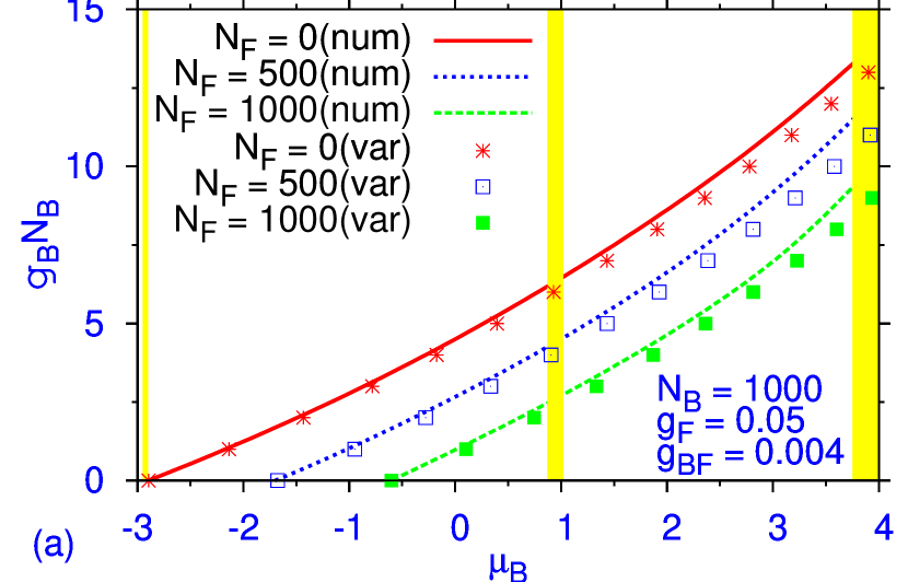
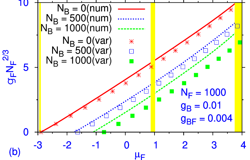
Figure 1: (Color online) The effective nonlinearity coefficients, $g_{B}N_{B}$ for bosons (a) and $g_{F}N_{F}^{2/3}$ for fermions (b), versus the chemical potentials of the boson and fermion components, $\mu_{B}$ and $\mu_{F}$, respectively, for families of the fundamental compact gap solitons in the first and second bandgaps of periodic potential $\epsilon\cos(2x)$ (numerical results are presented in this and other figures for $\epsilon=5$). As indicated in the figure, continuous curves and chains of symbols display, respectively, results obtained from the numerical solution (“num”) and variational approximation (“var”). Shaded vertical areas represent Bloch bands which separate the gaps.

In Fig. 2, typical shapes of the numerically found GSs are compared with their counterparts predicted by the VA at the following sets of parameter values: (a) $N_{F}=1000,N_{B}=500,g_{B}=0.01$; (b) $N_{F}=200,N_{B}=1000,g_{B}=0.001$; (c) $N_{F}=100,N_{B}=700,g_{B}=0.01$; (d) $N_{F}=100,N_{B}=500,g_{B}=0.01$. In all the four cases, $g_{F}=0.05$ and $g_{BF}=0.004$ are fixed. As written in the caption to Fig. 2, these parameters are chosen to represent four different cases, as concerns the location of the two chemical potentials, $\mu_{B}$ and $\mu_{F}$, in the two lowest bandgaps of the OL-induced linear spectrum: panels (a) and (d) represent the two-component solitons of the intra-gap type, while (b) and (c) represent inter-gap solitons, in terms of Ref. Arik . The agreement between the numerical and variational results is, again, quite noteworthy.

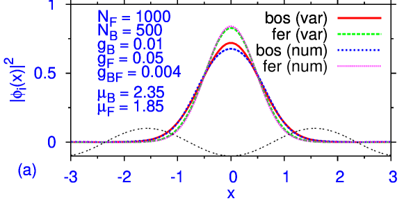
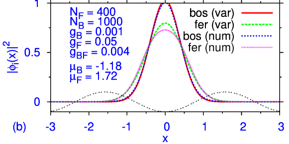
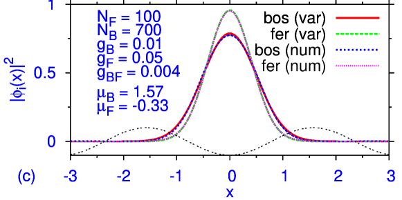
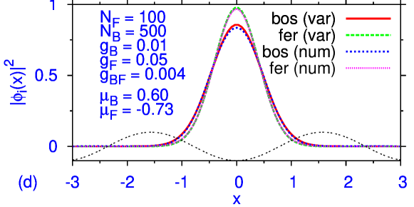
Figure 2: (Color online) Profiles of the probability density, $|\phi_{B,F}(x)|^{2}$ [subject to normalization $\int_{\infty}^{\infty}|\phi_{B,F}(x)|^{2}=1$] in the boson (“bos”) and fermion (“fer”) components of the fundamental gap solitons, in four different cases with (a) both components of the soliton having their chemical potentials, $\mu_{B}$ and $\mu_{F}$, in the second bandgap, (b) $\mu_{B}$ and $\mu_{F}$ in the first and second gaps, respectively; (c) vice versa to (b); (d) both components the first bandgap. In terms of Ref. Arik , the two-component gap solitons in panels (a) and (d) are of the intra-gap type, while the ones in (b) and (c) are inter-gap solitons. The thin dotted lines, here and in other figures, represent the OL potential, $\propto-\cos(2x)$.

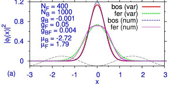
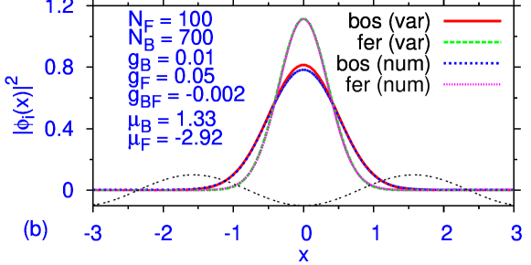
Figure 3: (Color online) Same as in Fig. 2 with (a) intraspecies attraction among bosonic atoms corresponding to a negative $g_{B}$ and (b) interspecies attraction between bosons and fermions corresponding to a negative $g_{BF}$. In (a) the bosonic GS is in the first bandgap and fermionic GS is in the second bandgap, in (b) vice versa to (a).

In Fig. 2 all the nonlinearities are taken as positive (repulsive). Another problem of interest is to investigate if GSs in the first two bandgaps can be found in both components when one of the nonlinearities ($g_{B}$ or $g_{BF}$) becomes attractive. (We recall that when $g_{BF}$ is sufficiently attractive, bright Bose and Fermi solitons can be generated without the OL potential Sadhan-BFsoliton . Such bright solitons will not have the chemical potential in the first two bandgaps and hence are not GSs.) We find that GSs in the first two bandgaps can indeed be found when either $g_{B}$ or $g_{BF}$ turns negative. We show typical results for this case in Fig. 3 (a) and (b), where we illustrate that by adjusting the parameters such GSs can be placed in the first or the second bandgap. These are inter-gap solitons. In addition intra-gap solitons can also be created in this case (not illustrated in Fig. 3.) The solitons shown in Fig. 3 are also stable, despite the fact that one nonlinearity coefficient changed its sign to an attractive value.

IV.2 Nonfundamental solitons

The fundamental GSs presented by Figs. 1 and 2 are compact objects with a nearly-Gaussian shape, trapped in a single cell of the OL. On the other hand, it is well known GSprediction that the GSs in self-repulsive repulsive BEC frequently demonstrate structures extended over many cells. Stable nonfundamental solitons featuring similar profiles can be found in the present model too, see examples in Fig. 4. They may be considered as bound complexes built of a central GS and additional pulses located in adjacent cells of the OL. Similar to the patterns shown Fig. 4, which extend over three lattice cells, at smaller values of the chemical potentials it is possible to find dynamically stable localized structures which are stretched still wider.

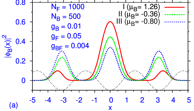
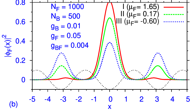
Figure 4: (Color online) Profiles labeled I, II, III [normalized according to $\int_{\infty}^{\infty}|\phi_{B,F}(x)|^{2}=1$] represent the bosonic (a) and fermionic (b) components of three distinct stable nonfundamental gap solitons, extended over several lattice cells, for the same parameters (except for $\mu_{B,F}$) as in Fig. 2(a). The corresponding values of the chemical potentials are indicated in the panels.

IV.3 Stability

The way the fundamental and nonfundamental GSs have been found, as a limit form to which solutions of underlying dynamical equations (13) and (14) relax at large values of $t$, strongly suggests that all these solutions are stable. Their stability was additionally tested by adding strong perturbations to them. It was thus verified that the entire families of the GSs presented above are stable, as well as the nonfundamental solitons displayed in Fig. 4. For example, the nonfundamental soliton labeled III in Fig. 4, after it was obtained as a steady state to which the evolution of a certain initial configuration converged, was suddenly multiplied by a perturbing factor, $\phi_{B,F}(x)\rightarrow 1.1\phi_{B,F}(x)$. The perturbed solution demonstrates oscillations without any onset of instability, as shown in Fig. 5.

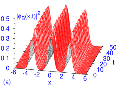
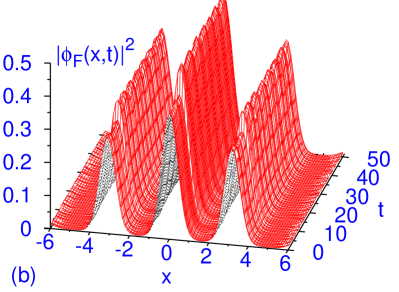
Figure 5: (Color online) The evolution of the boson (a) and fermion (b) components of the nonfundamental gap soliton, labeled III in Figs. 4, with $\mu_{B}=-0.80$ and $\mu_{F}=-0.60$. A rather strong perturbation was applied to the soliton at $t=10$, in the form of $\phi_{B,F}(x)\rightarrow 1.1\phi_{B,F}(x)$. The perturbed soliton remains stable as long as the simulation was running.

A typical example of the stability test for fundamental GSs is presented in Fig. 6, for the soliton shown in Fig. 2(a). At $t=10$, it was also “shaken”, multiplying it by factor $1.1$. The subsequent evolution makes the absence of any instability evident.

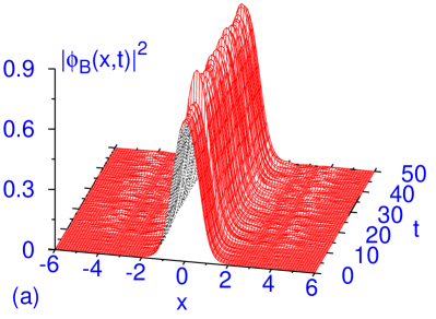
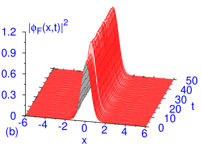
Figure 6: (Color online) The same stability test as shown in Fig. 5 for the fundamental soliton from Fig. 2.

V Conclusion

We have studied the possibility of generation of one-dimensional GSs (gap solitons) in a Bose-Fermi mixture trapped in a periodic OL potential, assuming that the bosons are in the BEC phase, and fermions are condensed into the BCS superfluid. A dynamical model of the mixture was derived from the system’s Lagrangian. The resultant coupled equations feature the cubic nonlinearity in the boson component, and the nonlinear term of power 7/3 in the equation for the fermion order parameter, with a cubic coupling between the equations, all the nonlinearities being repulsive.

Families of solutions for compact GSs, trapped, essentially, in the single lattice cell, were obtained by means of the VA (variational approximation) based on the Gaussian ansatz, and in the numerical form, in the two lowest bandgaps of the OL-induced spectrum. For a wide range of values of the interaction strengths and numbers of boson and fermions in the mixture, the VA predictions for the GS profiles and their chemical potentials agree very well with the respective numerical results. The GS families include both intra- and inter-gap solitons, with the chemical potentials of the boson and fermion components falling, respectively, in the same or different bandgaps. In addition to the fundamental GSs, we have also found (in the numerical form) nonfundamental localized structures, extended over several lattice sites. The entire families of the fundamental GSs, as well as the nonfundamental extended states, were checked to be robust against strong perturbations.

This work can be naturally extended in various directions. One possibility is to look for GSs in 2D and 3D models of the same type, study the possibility of the existence and stability of the two-component boson-fermion gap solitons and investigate their properties. Another perspective direction would be to study gap solitons in a boson-fermion mixture with mixed repulsive-attractive interactions in a systematic form, while in this paper we gave only a few examples. One can also seek for mixed bound states, in which the boson component belongs to the semi-infinite gap, while the fermionic chemical potential still belongs to a finite bandgap and vice versa. Lastly, it may happen that the coefficients which couple the bosons and fermions to the OL have opposite signs (one species is red-detuned, while the other one feels blue detuning), that may give rise to nontrivial stability limits for two-components GSs.

Here we used a set of mean-field equations for the study of GSs in Bose-Fermi mixtures. A rigorous treatment of this problem might be performed using a many-body Slater-determinant wave function Mario , as, for example, in the case of many-electron scattering ps .

- (1) C. Pethick and H. Smith. Bose-Einstein Condensation in Dilute Gases (Cambridge University Press: Cambridge, 2002); L. P. Pitaevskii and S. Stringari. Bose-Einstein Condensation (Clarendon Press: Oxford and New York, 2003).
- (2) B. DeMarco and D. S. Jin, Science 285, 1703 (1999).
- (3) K. M. O’Hara, S. L. Hemmer, M. E. Gehm, S. R. Granade, and J. E. Thomas, Science 298, 2179 (2002).
- (4) F. Schreck, L. Khaykovich, K. L. Corwin, G. Ferrari, T. Bourdel, J. Cubizolles, and C. Salomon, Phys. Rev. Lett. 87, 080403 (2001); A. G. Truscott, K. E. Strecker, W. I. McAlexander, G. B. Partridge, and R. G. Hulet, Science 291, 2570 (2001).
- (5) Z. Hadzibabic, C. A. Stan, K. Dieckmann, S. Gupta, M. W. Zwierlein, A. Gorlitz, and W. Ketterle, Phys. Rev. Lett. 88, 160401 (2002).
- (6) G. Modugno, G. Roati, F. Riboli, F. Ferlaino, R. J. Brecha, and M. Inguscio, Science 297, 2240 (2002).
- (7) G. Roati, F. Riboli, G. Modugno, and M. Inguscio, Phys. Rev. Lett. 89, 150403 (2002).
- (8) K. E. Strecker, G. B. Partridge, and R. G. Hulet, Phys. Rev. Lett. 91, 080406 (2003); Z. Hadzibabic, S. Gupta, C. A. Stan, C. H. Schunck, M. W. Zwierlein, K. Dieckmann, and W. Ketterle, ibid. 91, 160401 (2003).
- (9) R. Roth, Phys. Rev. A 66, 013614 (2002); R. Roth and H. Feldmeier, ibid. 65, 021603(R) (2002); T. Miyakawa, T. Suzuki, and H. Yabu, ibid. 64, 033611 (2001); X.-J. Liu, M. Modugno, and H. Hu, ibid. 68, 053605 (2003); X.-J. Liu and H. Hu, ibid. 67, 023613 (2003); K. Mølmer, Phys. Rev. Lett. 80, 1804 (1998).
- (10) M. Modugno, F. Ferlaino, F. Riboli, G. Roati, G. Modugno, and M. Inguscio, Phys. Rev. A 68, 043626 (2003).
- (11) P. Capuzzi, A. Minguzzi, and M. P. Tosi, Phys. Rev. A 69, 053615 (2004); 68, 033605 (2003); 67, 053605 (2003).
- (12) S. K. Adhikari, Phys. Rev. A 70, 043617 (2004).
- (13) J. R. Schrieffer, Theory of Superconductivity (W. A. Benjamin, Reading, 1964); M. Tinkham, Introduction to Superconductivity, 2nd Ed. (McGraw Hill, New York, 1996); A. L. Fetter A L and J. D. Walecka, Quantum Theory of Many Particle Systems (McGraw Hill, New York, 1971).
- (14) C. Chin, M. Bartenstein, A, Altmeyer, S. Riedl, S. Jochim, J. H. Denschlag, and R. Grimm, Science 305, 1128 (2004); T. Bourdel, L. Khaykovich, J. Cubizolles, J. Zhang, F. Chevy, M. Teichmann, L. Tarruell, S. J. J. M. F. Kokkelmans, and C. Salomon, Phys. Rev. Lett. 93, 050401 (2004); G. B. Partridge, K. E. Strecker, R. I. Kamar, M. W. Jack, and R. G. Hulet, ibid. 95, 020404 (2005).
- (15) M. Greiner, C. A. Regal, and D. S. Jin, Nature 426, 537 (2003); C. A. Regal, M. Greiner, and D. S. Jin, Phys. Rev. Lett. 92, 040403 (2004).
- (16) D. M. Eagles, Phys. Rev. 186, 456 (1969); A. J. Leggett, J. Phys. (Paris) Colloq. 41, C7-19 (1980); P. Nozières and S. Schmitt-Rink, J. Low Temp. Phys. 59, 195 (1985).
- (17) Y. Ohashi and A. Griffin, Phys. Rev. Lett. 89, 130402 (2002); Phys. Rev. A 67, 033603 (2003); ibid. 67, 063612 (2003); H. Hu, A. Minguzzi, X. J. Liu, and M. P. Tosi Phys. Rev. Lett 93, 190403 (2004); D. E. Sheehy and L. Radzihovsky, ibid. 96, 060401 (2006); C. H. Pao, S. T. Wu, and S. K. Yip, Phys. Rev. B 73, 132506 (2006); V. Gurarie and L. Radzihovsky, Ann. Phys. (NY) 322, 2 (2007).
- (18) C. A. Regal, and D. S. Jin, Adv. At. Mol. Opt. Phys. 54, 1 (2007).
- (19) S. K. Adhikari, M. de Llano, F. J. Sevilla, M. A. Solis, and J. J. Valencia, Physica C 453, 37 (2007).
- (20) K. E. Strecker, G. B. Partridge, A. G. Truscott and R. G. Hulet, Nature 417, 150 (2002); L. Khaykovich, F. Schreck, G. Ferrari, T. Bourdel, J. Cubizolles, L. D. Carr, Y. Castin, and C. Salomon, Science 256, 1290 (2002); V. M. Pérez-García, H. Michinel, and H. Herrero, Phys. Rev. A 57 , 3837 (1998).
- (21) S. L. Cornish, S. T. Thompson and C. E. Wieman, Phys. Rev. Lett. 96, 170401 (2006).
- (22) K. E. Strecker, G. B. Partridge, A. G. Truscott, and R. G. Hulet, New J. Phys. 5, 73 (2003); V. A. Brazhnyi and V. V. Konotop, Mod. Phys. Lett. B 18, 627 (2004); F. Kh. Abdullaev, A. Gammal, A. M. Kamchatnov, and L. Tomio, Int. J. Mod. Phys. B 19, 3415 (2005); F. Dalfovo, S. Giorgini, L. P. Pitaevskii, and S. Stringari, Rev. Mod. Phys. 71, 463 (1999); V. I. Yukalov, Laser Phys. Lett. 1, 435 (2004); A. Minguzzi, S. Succi, F. Toschi, M. P. Tosi, and P. Vignolo, Phys. Rep. 395, 223 (2004).
- (23) T. Karpiuk, K. Brewczyk, S. Ospelkaus-Schwarzer, K. Bongs, M. Gajda, and K. Rzazewski, Phys. Rev. Lett. 93, 100401 (2004); T. Karpiuk, M. Brewczyk, and K. Rzazewski, Phys. Rev. A 73, 053602 (2006).
- (24) S. K. Adhikari, Phys. Rev. A 72, 053608 (2005).
- (25) S. K. Adhikari, J. Phys. A 40, 2673 (2007); Europhys. J. D 40, 157 (2006).
- (26) G. L. Alfimov, V. V. Konotop, and M. Salerno, Europhys. Lett. 58, 7 (2002); B. B. Baizakov, V. V. Konotop, and M. Salerno, J. Phys. B 35, 51015 (2002); P. J. Y. Louis, E. A. Ostrovskaya, C. M. Savage, and Y. S. Kivshar, Phys. Rev. A 67, 013602 (2003).
- (27) K. M. Hilligsøe, M. K. Oberthaler, and K.-P. Marzlin, Phys. Rev. A 66, 063605 (2002); D. E. Pelinovsky, A. A. Sukhorukov and Y. S. Kivshar, Phys. Rev. E 70, 036618 (2004).
- (28) F. K. Abdullaev and M. Salerno, Phys. Rev. A 72, 033617 (2005).
- (29) G. L. Alfimov, V. V. Konotop, and P. Pacciani, Phys. Rev. A 75, 023624 (2007).
- (30) A. Gubeskys, B. A. Malomed, and I. M. Merhasin, Phys. Rev. A 73, 023607 (2006).
- (31) T. Mayteevarunyoo and B. A. Malomed, Phys. Rev. A 74, 033616 (2006).
- (32) B. J. Dabrowska-Wüster, E. A. Ostrovskaya, T. J. Alexander, and Y. S. Kivshar, Phys. Rev. A 75, 023617 (2007).
- (33) B. Eiermann, Th. Anker, M. Albiez, M. Taglieber, P. Treutlein, K.-P. Marzlin, and M. K. Oberthaler, Phys. Rev. Lett. 92, 230401 (2004).
- (34) O. Morsch and M. Oberthaler, Rev. Mod. Phys. 78, 179 (2006).
- (35) M. Matuszewski, W. Królikowski, M. Trippenbach, and Y. S. Kivshar, Phys. Rev. A 73, 063621 (2006).
- (36) T. Anker, M. Albiez, R. Gati, S. Hunsmann, B. Eiermann, A. Trombettoni, and M. K. Oberthaler, Phys. Rev. Lett. 94, 020403 (2005).
- (37) T. J. Alexander, E. A. Ostrovskaya, and Y. S. Kivshar, Phys. Rev. Lett. 96, 040401(2006).
- (38) P. G. Kevrekidis, B. A. Malomed, D. J. Frantzeskakis, A. R. Bishop, H. E. Nistazakis, and R. Carretero-González, Math. Comp. Sim. 69, 334 (2005).
- (39) V. M. Pérez-García and J. B. Beitia, Phys. Rev. A 72, 033620 (2005); S. K. Adhikari, Phys. Lett. A 346, 179 (2005).
- (40) M. Salerno, Phys. Rev. A 72, 063602 (2005).
- (41) S. K. Adhikari, Phys. Rev. A 73, 043619 (2006); S. K. Adhikari and B. A. Malomed, Phys. Rev. A 74, 053620 (2006).
- (42) S. K. Adhikari and L. Salasnich, Phys. Rev. A 75, 053603 (2007).
- (43) S. K. Adhikari, New J. Phys. 8, 258 (2006).
- (44) S. K. Adhikari, Phys. Rev. A 70, 043617 (2004).
- (45) V. M. Pérez-García, H. Michinel, J. I. Cirac, M. Lewenstein and P. Zoller, Phys. Rev. A 56 1424 (1997); B. A. Malomed, in Progress in Optics, vol. 43, p. 71 (ed. by E. Wolf: North-Holland, Amsterdam, 2002).
- (46) K. Huang and C. N. Yang, Phys. Rev. 105, 767 (1957).
- (47) T. D. Lee and C. N. Yang, Phys. Rev. 105, 1119 (1957).
- (48) N. Manini and L. Salasnich, Phys. Rev. A 71, 033625 (2005).
- (49) S. K. Adhikari and B. A. Malomed, Eur. Phys. Lett. 79, 50003 (2007).
- (50) L. Salasnich, Laser Phys. 12, 198 (2002); L. Salasnich, A. Parola, and L. Reatto, Phys. Rev. A 65, 043614 (2002); L. Salasnich and B. A. Malomed, Phys. Rev. A 74, 053610 (2006).
- (51) A. E. Muryshev, G. V. Shlyapnikov, W. Ertmer, K. Sengstock, and M. Lewenstein, Phys. Rev. Lett. 89, 110401 (2002); L. Khaykovich and B. A. Malomed, Phys. Rev. A 74, 023607 (2006); S. De Nicola, B. A. Malomed, and R. Fedele, Phys. Lett. A 360, 164 (2006).
- (52) S. K. Adhikari and P. Muruganandam, J. Phys. B 35, 2831 (2002); P. Muruganandam and S. K. Adhikari, ibid. 36, 2501 (2003); S. K. Adhikari, Phys. Rev. A 69, 063613 (2004).
- (53) P. K. Biswas and S. K. Adhikari, J. Phys. B 33, 1575 (2000); Chem. Phys. Lett. 317, 129 (2000).