Limit curve theorems in Lorentzian geometry

Abstract

The subject of limit curve theorems in Lorentzian geometry is reviewed. A general limit curve theorem is formulated which includes the case of converging curves with endpoints and the case in which the limit points assigned since the beginning are one, two or at most denumerable. Some applications are considered. It is proved that in chronological spacetimes, strong causality is either everywhere verified or everywhere violated on maximizing lightlike segments with open domain. As a consequence, if in a chronological spacetime two distinct lightlike lines intersect each other then strong causality holds at their points. Finally, it is proved that two distinct components of the chronology violating set have disjoint closures or there is a lightlike line passing through each point of the intersection of the corresponding boundaries.

1 Introduction

The limit curve theorems are surely one of the most fundamental tools of Lorentzian geometry. Their importance is certainly superior to that of analogous results in Riemannian geometry because in Lorentzian manifolds the curves may have a causal character, and hence it is particularly important to establish whether two points can be connected by a causal, a timelike or a lightlike curve.

The limit curve methods are so powerful and their range of applicability is so wide that often the application of a limit curve argument comes as the very first step in order to reach a desired result. In some sense the application of a limit curve theorem may be called a “brute force method”, a method which sometimes can be replaced by more elegant arguments but whose effectiveness can hardly be denied.

The proofs of this kind of results is often lengthy, and for this reason it is important to have them stated in a sufficiently general and informative way. Otherwise, the risk for the researcher is that of being forced to rebuild a slightly more general statement, all over again, any time a modification or an improvement is needed. Unfortunately, in my opinion, the limit curve theorems have not been stated with sufficient generality and as a researcher I have indeed experienced the above problem. The basic results so far available on limit curves are scattered across different books and research articles, with versions that rely on different conventions. Moreover, and most importantly, the statements of those results do not take full advantage of the powerful methods used in the proofs so that there is in fact enough room for interesting improvements.

The aim of this work is to comment and make some order on the results that have appeared in the literature, and to produce a version which should be able to capture most of the information that a limit curve theorem should give. In this way my hope is to make a service to those researchers who use limit curve theorems in Lorentzian geometry, and who want to rely on a general result with a detailed proof.

The changes experienced by the limit curve theorems in the last decades are worth knowing. I give a brief account which may help to understand in which sense the version given in this work is stronger or includes the previous formulations. I will translate the different versions in the notations of this work. Some technicalities will clarify in what follows. Note that the curves considered are always future-directed so that this adjective is omitted throughout the work.

A first version of limit curve theorem is theorem 6.2.1 of Hawking and Ellis [8]

Let $\gamma_{n}$ be an infinite sequence of continuous causal curves which are (past, future) inextendible. If $x$ is a limit point of $\gamma_{n}$, then through $x$ there is continuous causal curve which is (resp. past, future) inextendible and which is a limit curve of the $\gamma_{n}$.

This formulation has some weak points that I am going to comment.

• It uses a weak version of “limit curve” definition.

• The convergence obtained does not allow to apply results on the upper semi-continuity of the length functional unless strong causality is added.

• It does not include the case of curves with both endpoints, nor it includes the case in which the limit event ($x$ above) is not unique.

The first weak point comes from the particular definition of limit curve used in [8, Sect. 6.2]. They define $\sigma$ to be a limit curve of $\sigma_{n}$ if there is a (distinguishing) subsequence $\sigma_{m}$ such that for any $x\in\sigma$, every neighborhood of $x$ intersects an infinite number of $\sigma_{m}$ ($x$ is distinguished by $\sigma_{m}$).

In Beem et al. [3, Def. 3.28] a different definition is given where an infinite number is replaced by all but a finite number. There are simple examples of limit curves according to the definition of [8] which are not limit curves according to [3]. Thus the limit curve theorem by Beem et al. is stronger than that by Hawking and Ellis. Also, the theorem [3, Prop. 3.34] on the almost equivalence between the limit curve convergence and the $C^{0}$ convergence in strongly causal spacetimes does not hold with the definition of limit curve given in [8].

Although the version given in Beem et al. [3, Prop. 3.31] solved the problem (i), the formulation was pretty much similar to that by Hawking and Ellis. In particular in applications one often has to deal with limit curves situations in which one would like to apply the upper semi-continuity for the length functional. It was known, see Penrose’s book [15], that though the limit curve convergence was not enough in order to guarantee the upper semi-continuity of the length functional, at least under strong causality the $C^{0}$ convergence was indeed sufficient. Moreover, it was known that in strongly causal spacetimes the $C^{0}$ convergence is actually almost equivalent to the limit curve convergence in a sense clarified by Beem et al. in [3, Prop. 3.34]. In order to use the upper semi-continuity of the length functional in a limit curve theorem application one had then to assume the strong causality of the spacetime, pass through the $C^{0}$ convergence of the sequence, and apply the upper semi-continuity of length with respect to $C^{0}$ convergence as proved by Penrose [15] (Beem et al. [3, Remark 3.35] refer to it and to Busemann [4]). It was certainly a quite involved chain of implications, and the assumption of strong causality was a serious drawback.

Nevertheless, the proof given by Beem et al. [3, Prop. 3.31] contained an important improvement. By using the Arzela’s theorem, in a way analogous to what was done by Tonelli in the direct method of the calculus of variations [5], they were able to show that the limiting sequence parametrized with respect to the arc length of an auxiliary complete Riemannian metric, converges uniformly on compact subsets to a suitable parametrized limit curve. Galloway [7] noted that the uniform convergence on compact subsets was enough in order to guarantee the upper semi-continuity of the length functional, at least for curves restricted to a compact domain. This observation was of fundamental importance because from that moment on one could apply the limit curve theorem and the upper semi-continuity of the length functional with no need to assume additional causality requirements. In particular, the existence arguments for lines or rays, being based on limit maximizing sequences, strongly benefited from this observation.

From Beem et al. proof of the limit curve theorem, to Galloway’s observation, the technique of introducing an auxiliary complete Riemannian metric $h$ so as to parametrize the curves with respect to $h$-length became quite standard. The case in which the sequence is made of curves with endpoints, converging or diverging, was somewhat left aside and, though there were some important results in this direction (see [3, Theorem 8.13], [6, Lemma 1]), they did not appear as a single body of research together with the results on inextendible curves. The aim of this work is to formulate the limit curve theorem in a way sufficiently general to serve as a solid reference for future applications. In particular it will include the case of converging curves with endpoints.

We refer the reader to [12] for most of the conventions used in this work. In particular, we denote with $(M,g)$ a $C^{r}$ spacetime (connected, time-oriented Lorentzian manifold), $r\in\{2,\dots,\infty\}$ of arbitrary dimension $n\geq 2$ and signature $(-,+,\dots,+)$. Subsequences of a sequence of curves $\sigma_{n}$ are denoted with the same letter but changing the index. Thus we can say that $\sigma_{k}$ is a subsequence of $\sigma_{n}$.

In some places in order to save space and include in one single statement many different cases, the generic closed interval of the real line is denoted $[a,b]$, where $a$ can take the value $-\infty$ and $b$ can take the value $+\infty$ (thus $[0,+\infty]$ stands for $[0,+\infty)$). At the beginning of every lemma, theorem or definition it is clearly pointed out if this convention applies. Otherwise, $[a,b]$ denotes the usual compact interval, while the letter $I$ denotes the generic closed interval of the real line.

2 Some preliminary results

Recall that a continuous curve $\gamma:I\to M$, is causal if for every convex set $U$ and $t_{1},t_{2}\in I$, $t_{1}<t_{2}$, with $\gamma([t_{1},t_{2}])\subset U$, it is $\gamma(t_{1})<_{U}\gamma(t_{2})$ (see [8, 12]). A continuous causal curve can be shown to satisfy a local Lipschitz condition [3, Eq. 3.14], and hence to be almost everywhere differentiable. The same Lipschitz condition implies, in a suitable coordinate chart, the boundness of velocity at those points where it is defined. Note that the causality condition implies that there can’t be $t_{1},t_{2}\in I$, $t_{1}<t_{2}$, such that $\gamma([t_{1},t_{2}])=p\in M$, as it could be for a generic continuous curve.

The Lorentzian length $l(\gamma)$ of a continuous causal curve is defined as the greatest lower bound of the lengths of the interpolating causal geodesics [15]. Because of the almost everywhere differentiability, and of the local Lipschitz condition, this length can be calculated with the usual integral $l(\gamma)=\int_{I}\sqrt{-g(\dot{x},\dot{x})}\,{\rm d}t$.

Introduced on $M$ a Riemannian metric $h$, the Riemannian length $l_{0}(\gamma)$ of a continuous causal curve $\gamma:I\to M$ is defined, as usual, as the lower upper bound of the $h$-lengths of the interpolating $h$-geodesics. Due to the almost everywhere differentiability, and to the local Lipschitz condition, this length can be calculated with the usual integral $l(\gamma)=\int_{I}\sqrt{h(\dot{x},\dot{x})}\,{\rm d}t$. Since for a continuous causal curve there is no interval $[t_{1},t_{2}]$ such that $\gamma([t_{1},t_{2}])=p\in M$, the map $s(t)=l_{0}(\gamma|_{[t_{0},t]})$, $t_{0},t\in I$, is increasing and hence invertible. Thus any continuous causal curve can be reparametrized with respect to the Riemannian length with an invertible transformation.

The Lorentzian distance $d:M\times M\to[0,+\infty]$ is defined so that $d(x,z)$, $x,z\in M$, is the supremum over the Lorentzian lengths of the piecewise $C^{1}$ causal curves connecting $x$ to $z$ (piecewise $C^{1}$ can be replaced with “continuous”). Curiously, it is quite easy to prove that the Lorentzian distance is lower semi-continuous [3, Lemma 4.4], while the proof of the upper semi-continuity of the length functional is more involved. I give a version which is particularly suitable for our purposes. It improves the version of [15, theorem 7.5] in that the curves of the sequence as well as the limit curve may have or may not have endpoints (which if present do not need to be fixed) and strong causality is not assumed (thus embodying Galloway’s observation). The $C^{0}$ convergence is replaced with the convergence in the uniform topology, a small price to be paid in order to get rid of the strong causality assumption.

Recall that if $h$ is a Riemannian metric on $M$ and $d_{0}$ is the associated Riemannian distance then $\gamma_{n}:I\to M$ converges uniformly to $\gamma:I\to M$ if for every $\epsilon>0$ there is $N>0$, such that for $n>N$, and for every $t\in I$, $d_{0}(\gamma(t),\gamma_{n}(t))<\epsilon$. For the next application this definition is too restrictive and must be generalized to the case in which the domains of $\gamma_{n}$ differ.

Definition 2.1.

(In this definition $a_{n}$, $b_{n}$, $a$, $b$, may take an infinite value.) Let $h$ be a Riemannian metric on $M$ and let $d_{0}$ be the associated Riemannian distance. The sequence of curves $\gamma_{n}:[a_{n},b_{n}]\to M$ converges $h$-uniformly to $\gamma:[a,b]\to M$ if $a_{n}\to a$, $b_{n}\to b$, and for every $\epsilon>0$ there is $N>0$, such that for $n>N$, and for every $t\in[a,b]\cap[a_{n},b_{n}]$, $d_{0}(\gamma(t),\gamma_{n}(t))<\epsilon$.

The sequence of curves $\gamma_{n}:[a_{n},b_{n}]\to M$ converges $h$-uniformly on compact subsets to $\gamma:[a,b]\to M$ if for every compact interval $[a^{\prime},b^{\prime}]\subset[a,b]$, there is a choice of sequences $a^{\prime}_{n},b^{\prime}_{n}\in[a_{n},b_{n}]$, $a^{\prime}_{n}<b^{\prime}_{n}$, such that $a^{\prime}_{n}\to a^{\prime}$, $b^{\prime}_{n}\to b^{\prime}$, and for any such choice $\gamma_{n}|_{[a^{\prime}_{n},b^{\prime}_{n}]}$ converges $h$-uniformly to $\gamma|_{[a^{\prime},b^{\prime}]}$.

Remark 2.2.

Clearly, if $\gamma_{n}:[a_{n},b_{n}]\to M$ converges $h$-uniformly to $\gamma:[a,b]\to M$ then $\gamma_{n}$ converges $h$-uniformly on compact subsets to $\gamma$. Conversely, if $\gamma_{n}:[a_{n},b_{n}]\to M$ converges $h$-uniformly on compact subsets to $\gamma:[a,b]\to M$, $[a,b]$ is compact and $a_{n}\to a$, $b_{n}\to b$, then $\gamma_{n}$ converges $h$-uniformly to $\gamma$.

Remark 2.3.

Actually, the $h$-uniform convergence on compact subsets is independent of the Riemannian metric $h$ chosen. The reason is that if the domain of $\gamma:[a,b]\to M$ is compact then the same is true for its image and it is possible to find a open set of compact closure $A$, containing $\gamma([a,b])$. Then on $\bar{A}$, given a different Riemannian metric $h^{\prime}$, there are constants $m$ and $M$ such that $mh^{\prime}<h<Mh^{\prime}$.

Theorem 2.4.

Let $\gamma:[a,b]\to M$, be a continuous causal curve in the spacetime $(M,g)$ and let $h$ be a Riemannian metric on $M$.

• If the sequence of continuous causal curves $\gamma_{n}:[a,b]\to M$ converges $h$-uniformly to $\gamma$, then $\limsup l(\gamma_{n})\leq l(\gamma)$.

• If the sequence of continuous causal curves $\gamma_{n}:[a_{n},b_{n}]\to M$ converges $h$-uniformly to $\gamma$ and the curves $\gamma_{n}$ are parametrized with respect to $h$-length, then $\limsup l(\gamma_{n})\leq l(\gamma)$. Moreover, $\gamma_{n}$ converges to $\gamma$ in the $C^{0}$ topology and for every sequence $t_{n}\in[a_{n},b_{n}]$, $t_{n}\to t\in[a,b]$, it is $\gamma_{n}(t_{n})\to\gamma(t)$.

Proof.

Proof of (a). Given $\varepsilon>0$ a partition of $[a,b]$ can be found into intervals $[t_{1},t_{i+1}]$, $1\leq i\leq m-1$, $t_{i}\in[a,b]$, $t_{1}=a$, $t_{m}=b$, $t_{i}<t_{i+1}$, such that the interpolating geodesic $\eta$ passing through the events $x_{i}=\gamma(t_{i})$ has a length $l(\eta)\leq l(\gamma)+\varepsilon/2$, and there are convex sets $U_{i}$, $1\leq i\leq m-1$, covering $\gamma$ such that $\gamma|_{[t_{i},t_{i+1}]}\subset U_{i}$ (recall the length definition). In particular $x_{i}\in U_{i-1}\cap U_{i}$.

For every $i$ let events $y_{i},z_{i}\in U_{i-1}\cap U_{i}$ be chosen such that $y_{i}\ll_{U_{i}}x_{i}\ll_{U_{i-1}}z_{i}$. Thanks to the smoothness of the exponential map [14, Lemma 5.9] the Lorentzian distance $d_{i}:U_{i}\times U_{i}\to[0,+\infty]$ is finite and continuous for each $i$. Thus the events $y_{i},z_{i+1}\in U_{i}$ can be chosen close enough to $x_{i}$ and $x_{i+1}$ so that $d_{i}(y_{i},z_{i+1})<d_{i}(x_{i},x_{i+1})+\varepsilon/(2m)$. Since the image of $\gamma$ is compact and the convergence is uniform, it is possible to find $N>0$, such that for $n>N$, $\gamma_{n}\subset A=\bigcup^{m-1}_{i=1}U_{i}$ and $\gamma_{n}(t_{i})\in I_{U_{i}}^{+}(y_{i})\cap I_{U_{i-1}}^{-}(z_{i})$ for $2\leq i\leq m-1$, $\gamma_{n}(t_{1})\in I_{U_{1}}^{+}(y_{1})$, $\gamma_{n}(t_{m})\in I_{U_{i-1}}^{-}(z_{m})$. The curves $\gamma_{n}$ split into curves $\gamma_{n}^{i}=\gamma_{n}|_{[t_{i},t_{i+1}]}$ contained in $U_{i}$. Now, note that the curve $\gamma^{i}_{n}$ can be considered as the segment of a longer causal curve that connects $y_{i}$ to $z_{i+1}$ entirely contained in $U_{i}$, thus $l(\gamma^{i}_{n})\leq d_{i}(y_{i},z_{i+1})$. Finally,

$$l(\gamma_{n})\leq\sum_{i=1}^{m-1}d(y_{i},z_{i+1})\leq\sum_{i=1}^{m-1}d_{i}(x_{i},x_{i+1})+\frac{\varepsilon}{2}=l(\eta)+\frac{\varepsilon}{2}\leq l(\gamma)+\varepsilon.$$

Proof of (b). Given a compact $C$, there is a constant $M>0$ such that $-g<M^{2}h$. Indeed, since $(M,g)$, by definition of spacetime, is time orientable there is a global normalized timelike vector field $v$, $g(v,v)=-1$. Let $\eta=g(\cdot,v)$ be the associated 1-form and define $g^{\perp}$ of signature $(0,+,\ldots,+)$ so that, $g=-\eta\otimes\eta+g^{\perp}$. The metric $h^{\prime}=\eta\otimes\eta+g^{\perp}$ is Riemannian and given a vector $w$, $-g(w,w)=\eta(w)^{2}-g^{\perp}(w,w)\leq\eta(w)^{2}+g^{\perp}(w,w)=h^{\prime}(w,w)$. Since $C$ is compact there is $M>0$ such that $h^{\prime}<M^{2}h$.

Let $A$ be an open set of compact closure, $\bar{A}=C$, containing $\gamma$, and let $\Delta>0$ the Riemannian distance between $\gamma$ and $\dot{A}$. For every $a^{\prime},b^{\prime}\in(a,b)$, $a^{\prime}<b^{\prime}$, $|b-b^{\prime}|<\Delta/2$, $|a-a^{\prime}|<\Delta/2$, it is, for sufficiently large $n$, $[a^{\prime},b^{\prime}]\subset[a_{n},b_{n}]$, thus if the curves are restricted to the interval $[a^{\prime},b^{\prime}]$ (a) holds, $\limsup l(\gamma_{n}|_{[a^{\prime},b^{\prime}]})\leq l(\gamma|_{[a^{\prime},b^{\prime}]})$. Because of uniform convergence for sufficiently large $n$, it holds $d_{0}(\gamma,\gamma_{n}([a^{\prime},b^{\prime}]))<\Delta/2$, and since $\gamma_{n}$ are parametrized with respect to $h$-length $d_{0}(\gamma_{n}(a^{\prime}),\gamma_{n}(a))\leq|a-a^{\prime}|$ and analogously for the future endpoint. Using the triangle inequality it follows that $\gamma_{n}$ is entirely contained in $A$ which proves the $C^{0}$ convergence. Also $l(\gamma_{n}|_{[a,a^{\prime}]})\leq{M}\,l_{0}(\gamma_{n}|_{[a,a^{\prime}]})={M}\,|a^{\prime}-a|$, and $l(\gamma_{n}|_{[b^{\prime},b]})\leq{M}\,|b-b^{\prime}|$, so that $l(\gamma_{n})\leq l(\gamma_{n}|_{[a^{\prime},b^{\prime}]})+{M}\,|a^{\prime}-a|+{M}\,|b-b^{\prime}|$, and finally $\limsup l(\gamma_{n})\leq\limsup l(\gamma_{n}|_{[a^{\prime},b^{\prime}]})+{M}\,|a^{\prime}-a|+{M}\,|b-b^{\prime}|\leq l(\gamma|_{[a^{\prime},b^{\prime}]})+{M}\,|a^{\prime}-a|+{M}\,|b-b^{\prime}|$. Using the arbitrariness of $a^{\prime}$ and $b^{\prime}$, $\limsup l(\gamma_{n})\leq l(\gamma)$.

Finally, consider the sequence $t_{n}\in[a_{n},b_{n}]$, $t_{n}\to t\in[a,b]$. Let $\epsilon>0$, recall that $\gamma$ is continuous, and take $t^{\prime}\in(a,b)$ sufficiently close to $t$ that $d_{0}(\gamma(t),\gamma(t^{\prime}))<\epsilon/4$ and $|t^{\prime}-t|\leq\epsilon/4$. For sufficiently large $n$, $t^{\prime}\in[a_{n},b_{n}]$, and because of convergence we can also assume $d_{0}(\gamma(t^{\prime}),\gamma_{n}(t^{\prime}))<\epsilon/4$. Moreover, if $n$ is sufficiently large $|t_{n}-t|<\epsilon/4$ and finally $d_{0}(\gamma(t),\gamma_{n}(t_{n}))\leq d_{0}(\gamma(t),\gamma(t^{\prime}))+d_{0}(\gamma(t^{\prime}),\gamma_{n}(t^{\prime}))+d_{0}(\gamma_{n}(t^{\prime}),\gamma_{n}(t_{n}))\leq\frac{1}{2}\epsilon+|t^{\prime}-t_{n}|\leq\epsilon$

∎

Lemma 2.5.

Let $h$ be a Riemannian metric on the spacetime $(M,g)$. Every event $x\in M$, admits a globally hyperbolic coordinate neighborhood $(V,x^{\mu})$ ($x^{0}=const.$ are Cauchy hypersurfaces for $V$) and a constant $K>0$ such that if $\gamma:I\to M$ is a continuous causal curve and $\gamma|_{[t_{1},t_{2}]}\subset V$ then $l_{0}(\gamma|_{[t_{1},t_{2}]})\leq K|x^{0}(\gamma(t_{2}))-x^{0}(\gamma(t_{1}))|$.

Proof.

Every event $x\in M$ admits arbitrary small globally hyperbolic neighborhoods [12], in particular inside a neighborhood $U\ni x$, of compact closure. The neighborhood admits coordinates $\{x^{\mu}\}$ so that $g^{+}=-({\rm d}x^{0})^{2}+\sum_{i}({\rm d}x^{i})^{2}$, is such that $g^{+}>g$ (for details see [12, Lemma 2.13]). Since $g^{+}>g$, $\gamma$ is causal with respect to $g^{+}$.

On the compact $\bar{V}$ consider the Riemannian metric $\tilde{h}=({\rm d}x^{0})^{2}+\sum_{i}({\rm d}x^{i})^{2}$, then there is a constant $M>0$ such that $h<M^{2}\tilde{h}$ on $\bar{V}$. Let $t_{2}>t_{1}$ such that $\gamma([t_{1},t_{2}])\subset V$. The $\tilde{h}$-length of $\gamma|_{[t_{1},t_{2}]}$ is the supremum of the lengths of the interpolating piecewise $C^{1}$ $\tilde{h}$-geodesics, which for sufficiently fine interpolation are necessarily $g^{+}$-causal. Using the condition of $g^{+}$-causality, calling $\sigma$ one of the interpolating geodesics of $\gamma|_{[t_{1},t_{2}]}$, it is easily seen that $\tilde{l}_{0}(\sigma)\leq\sqrt{2}\,|x^{0}(\sigma(t_{2}))-x^{0}(\sigma(t_{1}))|$, and taking the supremum over the interpolating geodesics, since the endpoints remain the same, $\tilde{l}_{0}(\gamma|_{[t_{1},t_{2}]})\leq\sqrt{2}\,|x^{0}(\gamma(t_{2}))-x^{0}(\gamma(t_{1}))|$, thus $K=\sqrt{2}\,M$.

∎

The next lemma had been proved, in one direction, in [3, Lemma 3.65] and in the other direction at the end of the proof of [3, Prop. 3.31]. This last step is given here a different, shorter proof.

Lemma 2.6.

Let $(M,g)$ be a spacetime and let $h$ be a complete Riemannian metric on $M$. A continuous causal curve $\gamma$ once parametrized with respect to $h$-length has a domain unbounded from above iff future inextendible and unbounded from below iff past inextendible.

Proof.

Let $(a,b)$ be the interior of a domain obtained by parametrizing the curve with respect to $h$-length, with possibly $b=+\infty$ and $a=-\infty$. Assume $\gamma$ future inextendible and let $p=\gamma(t)$, $t\in(a,b)$, and consider the balls $B_{n}(p)=\{q:d_{0}(p,q)\leq n\}$. They are compact because of the Hopf-Rinow theorem. If $\gamma|_{[t,b)}$ is not entirely contained in $B_{n}(p)$ for a certain $n$, then $b-t=l_{0}(\gamma|_{[t,b)})\geq n$ for all $n$, thus $b=+\infty$. Otherwise, $\gamma|_{[t,b)}$ is contained in a compact and there is a sequence $t_{k}\in(a,b)$, $t_{k}\to b$, such that $\gamma(t_{k})\to q$. But since $q$ can’t be a limit point there are $\bar{t}_{k}\in(a,b)$, $\bar{t}_{k}\to b$, such that $\gamma(\bar{t}_{k})\notin B_{1/n}(q)$ for a certain $n$. For sufficiently large $k$, $\gamma(t_{k})\in B_{1/(2n)}(q)$, and hence $\gamma|_{[t,b)}$ enters $B_{1/(2n)}(q)$ and escapes $B_{1/n}(q)$ infinitely often, and thus has infinite length, $b-t=l_{0}(\gamma|_{[t,b)})=+\infty$ $\Rightarrow b=+\infty$.

Assume $b=+\infty$ then if $\gamma$ has a future endpoint $x$ there is a globally hyperbolic coordinate neighborhood $V$, as given in lemma 2.5, and a constant $t\in(a,+\infty)$ such that $\gamma|_{[t,+\infty)}\subset V$. But there is also a constant $K>0$ such that for $n>t$, $1=l_{0}(\gamma|_{[n,n+1]})\leq K|x^{0}(\gamma(n+1))-x^{0}(\gamma(n))|$, thus it is impossible that $x^{0}(\gamma(n))\to x^{0}(x)$, and hence that $\gamma(n)\to x$. ∎

The proof of the next lemma is in part contained in [3, Prop. 3.31], however the original proof contained a gap that is fixed here.

Lemma 2.7.

Let $(M,g)$ be a spacetime and let $h$ be a Riemannian metric on $M$. If the continuous causal curves $\gamma_{n}:I_{n}\to M$ parametrized with respect to $h$-length converge $h$-uniformly on compact subsets to $\gamma:I\to M$ then $\gamma$ is a continuous causal curve.

Proof.

Let $\gamma([t_{1},t_{2}])\subset U$, $[t_{1},t_{2}]\subset I$, with $U$ ($g$-)convex neighborhood. Let $\Delta>0$ be the Riemannian distance between the compact $\gamma([t_{1},t_{2}])$ and the closed set $U^{C}$. By uniform convergence on compact subsets there are sequences $t_{1n},t_{2n}\in I_{n}$, such that $t_{1n}\to t_{1}$, $t_{2n}\to t_{2}$, and $\gamma_{n}|_{[t_{1n},t_{2n}]}$ converges $h$-uniformly to $\gamma|_{[t_{1},t_{2}]}$, in particular for large $n$, $\gamma_{n}|_{[t_{1n},t_{2n}]}$ has an image included in $U$. Thus, $\gamma_{n}(t_{1n})\leq_{U}\gamma_{n}(t_{2n})$, and because of theorem 2.4, case (b), $\gamma_{n}(t_{1n})\to\gamma(t_{1})$, $\gamma_{n}(t_{2n})\to\gamma(t_{2})$. Now, recall that $J^{+}_{U}$ is closed in a convex neighborhood, and hence $\gamma(t_{1})\leq_{U}\gamma(t_{2})$. It remains to prove that $\gamma(t_{1})\neq\gamma(t_{2})$ so that $\gamma(t_{1})<_{U}\gamma(t_{2})$ (the proof of [3, Prop. 3.31] lacks this part). Indeed, if $\gamma(t_{1})=\gamma(t_{2})$ then $\gamma(t)=\gamma(t_{1})$, for every $t\in[t_{1},t_{2}]$, otherwise there would be $\bar{t}\in[t_{1},t_{2}]$, $\gamma(t_{1})<_{U}\gamma(\bar{t})<_{U}\gamma(t_{1})$ which would violate the causality of $(U,g|_{U})$ (recall that every convex neighborhood is causal). Finally,

$$t_{2}-t_{1} =\limsup(t_{2n}-t_{1n})=\limsup{l}_{0}(\gamma_{n}|_{[t_{1n},t_{2n}]})$$

$$\leq K\,\limsup|x^{0}(\gamma_{n}(t_{2n}))-x^{0}(\gamma_{n}(t_{1n}))|=K|x^{0}(\gamma(t_{2}))-x^{0}(\gamma(t_{1}))|$$

thus if $t_{2}\neq t_{1}$ necessarily $\gamma(t_{2})\neq\gamma(t_{1})$.

∎

With slight modifications the next local result is contained in Lemma 1 of [2] (see also [1, Lemma 3.1]). $J^{+}_{S}$ denotes the Seifert causal relation [16, 10].

Lemma 2.8.

Let $(M,g)$ be a spacetime, and $p\in M$. Let $g_{n}\geq g$ be a sequence of metrics such that $g_{n+1}\leq g_{n}$, and assume that the metrics $g_{n}$, regarded as sections of the bundle $T^{*}M\otimes T^{*}M\to M$, converge pointwisely to the metric $g$. There is a $g$-convex neighborhood $V\ni p$, contained, for all $n$ in $g_{n}$-convex neighborhoods $V_{n}$, such that if $(x_{n},z_{n})\in J^{+}_{(V,g_{n})}$, and $(x_{n},z_{n})\to(x,z)$, then $(x,z)\in J^{+}_{(V,g)}$. In particular $J^{+}_{S(V,g)}=J^{+}_{(V,g)}$.

Corollary 2.9.

Let $(M,g)$ be a spacetime and let $h$ be a Riemannian metric on $M$. Let $g_{n}\geq g$ be a sequence of metrics such that $g_{n+1}\leq g_{n}$, and assume that the metrics $g_{n}$, regarded as sections of the bundle $T^{*}M\otimes T^{*}M\to M$, converge pointwisely to the metric $g$. A curve which is a continuous $g_{n}$-causal curve for every $n$ is actually a continuous $g$-causal curve.

In particular, let $\gamma_{n}:I_{n}\to M$ be a continuous $g_{n}$-causal curve parametrized with respect to $h$-length, and assume that the sequence $\gamma_{n}$ converges $h$-uniformly on compact subsets to $\gamma:I\to M$, then $\gamma$ is a continuous $g$-causal curve.

Proof.

We have to prove that for every ($g$-)convex set $U$, and interval $[t_{1},t_{2}]\subset I$, such that $\gamma([t_{1},t_{2}])\subset U$, it is $\gamma(t_{1})<_{(U,g)}\gamma(t_{2})$. To this end it is sufficient to prove the statement with $U$ replaced with the set $V$ whose properties are given by lemma 2.8. Indeed, $\gamma([t_{1},t_{2}])$ being compact can be covered with a finite number of such neighborhoods contained in $U$. Thus assume that $U$ has the properties of lemma 2.8, in particular it is $g$-convex and contained in $g_{n}$-convex sets $U_{n}$. Then $(\gamma(t_{1}),\gamma(t_{2}))\in J^{+}_{(U,g_{n})}$ and $\gamma(t_{1})\neq\gamma(t_{2})$, because $\gamma$ is continuous $g_{n}$-causal. Using the property of $U$ it follows $(\gamma(t_{1}),\gamma(t_{2}))\in J^{+}_{(U,g)}$, and $\gamma(t_{1})\neq\gamma(t_{2})$, hence $\gamma$ is continuous $g$-causal.

For every $k>0$, the sequence $\gamma_{n}$ for $n>k$ converges $h$-uniformly on compact subsets to $\gamma:I\to M$. Since all the causal curves are $g_{k}$-causal, the limit curve $\gamma$ is continuous $g_{k}$-causal by lemma 2.7, where $k$ is arbitrary, hence it is continuous $g$-causal by the previous observation. ∎

Remark 2.10.

The previous result is particularly important in connection with stable causality. It proves that in many cases the limit curve is actually $g$-causal though the limiting sequence is made of $g_{n}$-causal curves with $g_{n}\geq g$. Its main idea was successfully applied by Beem in [2, Theorem 2]. It is important to keep it in mind because, while the next limit curve theorems will be stated using sequences of curves which are causal with respect to the same metric $g$, the theorems can be easily generalized to the case contemplated by the previous lemma.

Definition 2.11.

A continuous causal curve $\gamma:I\to M$, is maximizing if, for every $t_{1},t_{2}\subset I$, $t_{1}<t_{2}$, $d(\gamma(t_{1}),\gamma(t_{2}))=l(\gamma|_{[t_{1},t_{2}]})$.

A sequence of continuous causal curves $\gamma_{n}:I_{n}\to M$, is limit maximizing if defined

$$\epsilon_{n}=\sup_{t_{1},t_{2}\in I_{n},t_{1}<t_{2}}[d(\gamma_{n}(t_{1}),\gamma_{n}(t_{2}))-l(\gamma_{n}|_{[t_{1},t_{2}]})]\geq 0,$$

it is $\lim_{n\to+\infty}\epsilon_{n}=0$.

In particular a maximizing causal curve is a geodesic without conjugated points, but for, possibly, the endpoints. If it is inextendible it is called a line, if it is future inextendible but has past endpoint it is called a future ray (and analogously in the past case).

The Lorentzian distance is not a conformal invariant function, as a consequence the property of being a line or a ray for a causal curve is not a conformal invariant property. An exception are the lightlike lines or rays, indeed they can be given the following equivalent conformal invariant definition.

Definition 2.12.

A lightlike line is a achronal inextendible continuous causal curve. A future lightlike ray is a achronal future inextendible continuous causal curve with a past endpoint (and analogously in the past case).

The next theorem extends a result by Eschenburg and Galloway [6] to the case of curves without both endpoints, their result being already an improvement with respect to [3, Prop. 8.2] which used strong causality.

Theorem 2.13.

Let $(M,g)$ be a spacetime and let $h$ be a Riemannian metric on $M$. If the sequence of continuous causal curves $\gamma_{n}:I_{n}\to M$ is limit maximizing, the curves are parametrized with respect to $h$-length and the sequence converges $h$-uniformly on compact subsets to the curve $\gamma:I\to M$, then $\gamma$ is a maximizing continuous causal curve. Moreover, given $[a,b]\subset I$ there are $[a_{n},b_{n}]\subset I_{n}$, such that $a_{n}\to a$, $b_{n}\to b$ and for any such choice

$$\lim l(\gamma_{n}|_{[a_{n},b_{n}]})=\lim d(\gamma_{n}(a_{n}),\gamma_{n}(b_{n}))=l(\gamma|_{[a,b]})=d(\gamma(a),\gamma(b)).$$ (1)

Proof.

The curve $\gamma$ is a continuous causal curve because of lemma 2.7. Let $[a,b]\subset I$, then there are $[a_{n},b_{n}]\subset I_{n}$, such that $a_{n}\to a$, $b_{n}\to b$, and $\gamma_{n}|_{[a_{n},b_{n}]}$ converges $h$-uniformly to $\gamma_{[a,b]}$. Since $d$ satisfies the reverse triangle inequality $d(\gamma_{n}(a_{n}),\gamma_{n}(b_{n}))-l(\gamma_{n}|_{[a_{n},b_{n}]})\leq\epsilon_{n}$, with $\epsilon_{n}\to 0$. Using case (b) of theorem 2.4 and the lower semi-continuity of the distance

$$d(\gamma(a),\gamma(b)) \leq\liminf d(\gamma_{n}(a_{n}),\gamma_{n}(b_{n}))\leq\limsup d(\gamma_{n}(a_{n}),\gamma_{n}(b_{n}))$$

$$\leq\limsup l(\gamma_{n}|_{[a_{n},b_{n}]})\leq l(\gamma|_{[a,b]})\leq d(\gamma(a),\gamma(b))$$

hence $d(\gamma(a),\gamma(b))=l(\gamma|_{[a,b]})$ which concludes the proof. ∎

Remark 2.14.

Given two converging sequences $x_{n}\to x$, $z_{n}\to z$, such that $x_{n}<z_{n}$ and $d(x_{n},z_{n})<+\infty$, it is always possible to construct a limit maximizing sequence of curves $\gamma_{n}:[a_{n},b_{n}]\to M$, $x_{n}=\gamma(a_{n})$, $z_{n}=\gamma(b_{n})$. This observation is particularly useful, since the existence of a limit maximizing sequence is the starting point from which many results on the existence of causal rays or lines are obtained. Sometimes, the sequence of endpoints may not satisfy $d(x_{n},z_{n})<+\infty$. In this case, provided the spacetime is strongly causal, it is still possible to construct a sort of limit maximizing sequence. The reader is referred to [3, Chap. 8] for details.

The next lemma develops an idea used by Eschenburg and Galloway in [6, Lemma 1].

Lemma 2.15.

Let $(M,g)$ be a spacetime and let $h$ be a complete Riemannian metric on $M$.

• If the continuous causal curve $\gamma:(a,b)\to M$ parametrized with respect to $h$-length, is such that $l(\gamma_{[t,b)})=+\infty$, for one (and hence every) $t\in(a,b)$ then $b=+\infty$ (and analogously in the past case).

• If the sequence of continuous causal curves $\gamma_{n}:(a_{n},b_{n})\to M$ parametrized with respect to $h$-length, is such that $l(\gamma|_{[t_{n},b_{n})})\to+\infty$, for a sequence $t_{n}\in(a_{n},b_{n})$, $t_{n}\to t$, such that $\gamma_{n}(t_{n})\to q\in M$, then $b_{n}\to+\infty$ (and analogously in the past case).

Proof.

Proof of (i). Let $p=\gamma(t)$, if $\gamma_{[t,b)}$ escapes every ball $B_{n}(p)$ necessarily $b-t=l_{0}(\gamma|_{[t,b)})=+\infty$, thus $b=+\infty$. Otherwise, the image of $\gamma_{[t,b)}$ is contained in a compact (Hopf-Rinow theorem) $C=B_{n}(p)$ for a suitable $n$. Given the compact $C$, there is a constant $M>0$ such that $-g<M^{2}h$ (see the proof of (b) theorem 2.4), then $b-t=l_{0}(\gamma|_{[t,b)})>M^{-1}l(\gamma|_{[t,b)})=+\infty$ which implies $b=+\infty$.

Proof of (ii). Assume not then there is a subsequence $\gamma_{k}$ such that $b_{k}<N$, for a suitable $N>0$. If for every $s>0$ only a finite number of $\gamma_{k}|_{[t_{k},b_{k})}$ is entirely contained in $B_{s}(q)$ necessarily $b_{k}-t_{k}=l_{0}(\gamma_{k}|_{[t_{k},b_{k})})\to+\infty$ which implies $b_{k}\to+\infty$ a contradiction. Thus there is subsequence $\gamma_{i}$ of $\gamma_{k}$ which is entirely contained in a compact $C=B_{s}(q)$ for a suitable $s>0$. But there is a constant $M>0$ such that $-g<M^{2}h$ on $C$, then $b_{i}-t_{i}=l_{0}(\gamma|_{[t_{i},b_{i})})>M^{-1}l(\gamma_{i}|_{[t_{i},b_{i})})\to+\infty$ which implies $b_{i}\to+\infty$, while $b_{i}<N$. The overall contradiction proves that $b_{n}\to+\infty$.

∎

Theorem 2.16.

Let $\gamma:[a,b]\to M$ be a causal curve such that $\gamma(a)=\gamma(b)$ then either (i) $\gamma^{\prime}(a)\propto\gamma^{\prime}(b)$ and $\gamma$ is obtained from the domain restriction of a closed lightlike line $\eta$ or (ii) $\gamma$ is entirely contained in the chronology violating set. Moreover, if $\gamma$ does not intersect the closure of the chronology violating set then (i) holds and $\eta$ is a complete geodesic.

Proof.

If $\gamma$ is not a achronal then there are points $p,q\in\gamma$ such that $p\ll q$. Take arbitrary $r\in\gamma$, since $\gamma$ is closed, $r\leq p$ and $q\leq r$, thus $r\leq p\ll q\leq r$, i.e. $r\ll r$, that is $r$ belongs to the chronology violating set. Thus $\gamma$ is achronal or (ii) holds. Assume (ii) does not hold. The achronality implies that $\gamma$ is a lightlike geodesic. Note that if $\gamma^{\prime}(a)\propto\gamma^{\prime}(b)$ does not hold then rounding the corner it is possible to find $p,q\in\gamma$ such that $p\ll q$. Thus if (ii) does not hold taking infinite rounds over $\gamma$ it is possible to obtain an achronal inextendible causal curve i.e. a lightlike line. The last statement follows from proposition 6.4.4 of [8]. ∎

3 The limit curve theorem

In the following limit curve theorem the sequence $\gamma_{n}$ is made of continuous causal curves parametrized with respect to $h$-length. The statement that the curves converge $h$-uniformly on every compact subset is a very powerful result that contains a lot of information. It is then natural to formulate the theorem so as to mention the role of the parametrization. Nevertheless, since the Riemannian length functional is lower semi-continuous but non upper semi-continuous the parametrization of the limit curve is not necessarily the natural $h$-length parametrization.

The theorem is quite lengthy, and at first its meaning may be difficult to grasp. However, in applications the reader may use the information on the converging sequence to select a particular case among those there considered. Case (1) and (2) can be regarded as particular cases of case (3). However, they are stated separately as they have some peculiarities which are particularly useful in applications.

Since the theorem deals with a sequence of curves possibly with endpoints, some additional mild requirements are required in order to guarantee that the sequence does not shrink to a single event and that the limit curve does indeed exist.

Theorem 3.1.

Let $(M,g)$ be a spacetime, and let $h$ be a complete Riemannian metric.

• [One converging sequence case] (here $a_{k}$, $b_{k}$, $a$, $b$, may take an infinite value.) Let $y$ be an accumulation point of a sequence of continuous causal curves. There is a subsequence parametrized with respect to $h$-length, $\gamma_{k}:[a_{k},b_{k}]\to M$, $0\in[a_{k},b_{k}]$, such that $\gamma_{k}(0)\to y$ and such that the next properties hold. There are $a\leq 0$ and $b\geq 0$, such that $a_{k}\to a$ and $b_{k}\to b$. If there is a neighborhood $U$ of $y$ such that only a finite number of $\gamma_{k}$ is entirely contained in $U$ (which happens iff $b>0$ or $a<0$) then there is a continuous causal curve $\gamma:[a,b]\to M$, $0\in[a,b]$, $y=\gamma(0)$, such that $\gamma_{k}$ converges $h$-uniformly on compact subsets to $\gamma$.

  In particular if $a>-\infty$, then $a_{k}>-\infty$ and $x_{k}=\gamma_{k}(a_{k})$ converges to $x=\gamma(a)$. Analogously, if $b<+\infty$, then $b_{k}<+\infty$, and $z_{k}=\gamma_{k}(b_{k})$ converges to $z=\gamma(b)$. If $a_{k}>-\infty$, $x_{k}=\gamma_{k}(a_{k})\to+\infty$ or $l(\gamma_{k}|_{[a_{k},0]})\to+\infty$ then $a=-\infty$, and if $b_{k}<+\infty$, $z_{k}=\gamma(b_{k})\to+\infty$ or $l(\gamma_{k}|_{[0,b_{k}]})\to+\infty$ then $b=+\infty$.

  All the mentioned parametrized curves, the sequence $\gamma_{k}$ and $\gamma$, are future inextendible iff their interval of definition is unbounded from above, and past inextendible iff their interval of definition is unbounded from below.

  Finally, if $\gamma_{k}$ is limit maximizing then $\gamma$ is maximizing.

• [Two converging sequences case] (here $b$ may take an infinite value.) Let $\gamma_{n}$ be a sequence of continuous causal curves with past endpoint $x_{n}$ and future endpoint $z_{n}$ such that $x_{n}\to x$, $z_{n}\to z$. There is a subsequence parametrized with respect to $h$-length denoted $\gamma^{x}_{k}:[0,b_{k}]\to M$, such that $x_{k}=\gamma^{x}_{k}(0)\to x$, $z_{k}=\gamma^{x}_{k}(b_{k})\to z$, a analogous reparametrized sequence of continuous causal curves $\gamma^{z}_{k}(t)=\gamma^{x}_{k}(t+b_{k})$, $\gamma^{z}_{k}:[-b_{k},0]\to M$, such that $x_{k}=\gamma^{z}_{k}(-b_{k})\to x$, $z_{k}=\gamma^{z}_{k}(0)\to z$, all such that the next properties hold. There is $b\geq 0$, such that $b_{k}\to b$. If there is a neighborhood $U$ of $x$ such that only a finite number of $\gamma_{k}$ is entirely contained in $U$ (which is true iff $b>0$ or if $x\neq z$ or if $x_{n}=z_{n}$) then there is a continuous causal curve $\gamma^{x}:[0,b]\to M$, $x=\gamma^{x}(0)$, and a continuous causal curve $\gamma^{z}:[-b,0]\to M$, $z=\gamma^{z}(0)$, such that $\gamma^{x}_{k}$ converges $h$-uniformly on compact subsets to $\gamma^{x}$, and $\gamma^{z}_{k}$ converges $h$-uniformly on compact subsets to $\gamma^{z}$.

  There are two cases,

  • $0<b<+\infty$, $\gamma^{z}(t)=\gamma^{x}(t+b)$, $\gamma^{x}(b)=z$, $\gamma^{z}(-b)=x$, so that $\gamma^{x}$ and $\gamma^{z}$ connect $x$ to $z$, they are one the reparameterization of the other and $\limsup l(\gamma^{x}_{k})\leq l(\gamma^{x})$,

  • $b=+\infty$, $\gamma^{x}$ is future inextendible, $\gamma^{z}$ is past inextendible and given $t^{x}\in[0,+\infty)$, $t^{z}\in(-\infty,0]$, there is $K(t^{x},t^{z})>0$ such that for $k>K$, $\gamma_{k}^{x}(t^{x})\leq\gamma_{k}^{z}(t^{z})$, in particular for every choice of $\bar{x}\in\gamma^{x}$ and $\bar{z}\in\gamma^{z}$, it is $(\bar{x},\bar{z})\in\bar{J}^{+}$. If $\gamma^{x}$ is not a lightlike ray then $\gamma^{z}\subset\bar{J}^{+}(x)$, and if $\gamma^{z}$ is not a lightlike ray then $\gamma^{x}\subset\bar{J}^{-}(z)$. If neither $\gamma^{x}$, nor $\gamma^{z}$ is a lightlike ray then $z\in I^{+}(x)$. If ($\gamma^{x}$ is not a lightlike ray or $\forall n$, $x_{n}=x$) and ($\gamma^{z}$ is not a lightlike ray or $\forall n$, $z_{n}=z$) then $\limsup l(\gamma_{k}^{x})\leq d(x,z)$. If the spacetime is non-totally imprisoning then the curves $\gamma_{n}$ are not all contained in a compact.

  If the curves $\gamma_{k}$ are not all contained in a compact or if $l(\gamma_{n})\to+\infty$ then $b=+\infty$.

  If $x=z$ and $b=+\infty$ then $\gamma=\gamma^{x}\circ\gamma^{z}$ is an inextendible limit (cluster) curve of $\gamma_{n}$, for every $\tilde{x},\tilde{z}\in\gamma$, it is $(\tilde{x},\tilde{z})\in\bar{J}^{+}$ and strong causality is violated at every point of $\gamma$. Moreover, if $\gamma$ is not a lightlike line then all but a finite number of the curves $\gamma_{k}^{x}$ intersect the chronology violating set.

  If $x=z$ and $0<b<+\infty$ then $\gamma^{x}$ is a closed continuous causal curve starting and ending at $x$. The curve $\gamma$ obtained making infinite rounds over $\gamma^{x}$ is inextendible and causality is violated at every point of $\gamma$. Moreover, either $\gamma$ is a lightlike line or it is entirely contained in the chronology violating set.

  Finally whether $x=z$ or not, if $\gamma_{n}$ is limit maximizing then both $\gamma^{x}$ and $\gamma^{z}$ are maximizing and if, moreover, $b=+\infty$ then $l(\gamma^{x})+l(\gamma^{z})\leq\limsup l(\gamma_{n})$. Thus, in this last case if $\limsup l(\gamma_{n})<+\infty$ then $\gamma^{x}$ and $\gamma^{z}$ are lightlike rays or one of them is an incomplete timelike ray.

• [general case] (here $a$, $b$, $a_{n}$, $b_{n}$, $a_{k}$, $b_{k}$, $a^{(i)}$, $b^{(i)}$, may take an infinite value.) Let $\gamma_{n}:[a_{n},b_{n}]\to M$ be a sequence of continuous causal curves parametrized with respect to $h$-length. Let $\{y^{(i)}\}$, $\{i\}=G\subset\mathbb{N}$, be a non-empty and at most numerable set of limit points for $\gamma_{n}$ (namely, every neighborhood of $y^{(i)}$ intersect all but a finite number of the curves $\gamma_{n}$). If $\limsup(b_{n}-a_{n})>0$ then there is a subsequence $\gamma_{k}$ of $\gamma_{n}$ such that $\lim(b_{k}-a_{k})$ exists, there are sequences $t^{(i)}_{k}\in[a_{k},b_{k}]$, $\gamma_{k}(t^{(i)}_{k})\to y^{(i)}$, the limits $\lim(a_{k}-t^{(i)}_{k})$, $\lim(b_{k}-t^{(i)}_{k})$ exist, there are continuous causal curves $\gamma^{(i)}:[a^{(i)},b^{(i)}]\to M$, $a^{(i)}=\lim(a_{k}-t^{(i)}_{k})$, $b^{(i)}=\lim(b_{k}-t^{(i)}_{k})$, $\gamma^{(i)}(0)=y^{(i)}$, such that the sequence $\gamma^{(i)}_{k}:[a_{k}-t^{(i)}_{k},b_{k}-t^{(i)}_{k}]\to M$, defined by $\gamma^{(i)}_{k}(t)=\gamma_{k}(t+t^{(i)}_{k})$, converges $h$-uniformly on compact subsets to $\gamma^{(i)}$. The curves $\gamma^{(i)}$ are past inextendible iff $a^{(i)}=-\infty$ and future inextendible iff $b^{(i)}=+\infty$.

  Given $i\neq j$, $i,j\in G$, there are only three possibilities. Either $t^{(i)}_{k}-t^{(j)}_{k}\to c^{(ij)}=-c^{(ji)}=const.$, in which case we write $(i)\sim(j)$, or $t^{(i)}_{k}-t^{(j)}_{k}\to\pm\infty$. In the first case, $\gamma^{(i)}$ and $\gamma^{(j)}$ are one the reparameterization of the other, $\gamma^{(i)}(t)=\gamma^{(j)}(t+c^{(ij)})$. If $t^{(i)}_{k}-t^{(j)}_{k}\to+\infty$ then for every $t^{(i)}\in[a^{(i)},b^{(i)}]$ and $t^{(j)}\in[a^{(j)},b^{(j)}]$, there is $K(t^{(j)},t^{(i)})$ such that for $k>K$, $\gamma^{(j)}_{k}(t^{(j)})\leq\gamma^{(i)}_{k}(t^{(i)})$, in particular for every $x^{(j)}\in\gamma^{(j)}$ and $x^{(i)}\in\gamma^{(i)}$, $(x^{(j)},x^{(i)})\in\bar{J}^{+}$, and analogously with the roles of $i$ and $j$ inverted if $t^{(i)}_{k}-t^{(j)}_{k}\to-\infty$.

  Finally, if $\gamma_{n}$ is limit maximizing then each $\gamma^{(i)}$ is maximizing and

  $$\sum_{G/\sim}l(\gamma^{(i)})\leq\limsup l(\gamma_{n}).$$

Proof.

The starting point is a limit curve lemma [7] [3, Lemma 14.2] whose proof is contained in the proof of [3, Prop. 3.31].

(Limit curve lemma) Let $\gamma_{n}:(-\infty,+\infty)\to M$, be a sequence of inextendible continuous causal curves parametrized with respect to $h$-length, and suppose that $y\in M$ is an accumulation point of the sequence $\gamma_{n}(0)$. There is a inextendible continuous causal curve $\gamma:(-\infty,+\infty)\to M$, such that $\gamma(0)=y$ and a subsequence $\gamma_{k}$ which converges $h$-uniformly on compact subsets to $\gamma$.

The concept of $h$-uniform convergence on compact subsets used in [3] is equivalent to that introduced in definition 2.1 if the curves of the sequence and the limit curve are defined in $(-\infty,+\infty)$. Thus the limit curve lemma holds also with the notations and definitions of this work. The idea is to extend each curve of the sequence into an inextendible continuous causal curve, apply the limit curve lemma and show that the limit curve, restricted to a suitable domain, is a limit curve for the unextended sequence.

• Proof of (1). Parametrize the sequence with respect to $h$-length and pass to a subsequence to get $\gamma_{n}:[a_{n},b_{n}]\to M$, $0\in[a_{n},b_{n}]$, $\gamma_{n}(0)\to y$. Pass to a subsequence $\gamma_{i}$ so that there are $a\leq 0$, and $b\geq 0$, such that $a_{i}\to a$, $b_{i}\to b$. If there is a neighborhood $U$ of $y$ such that only a finite number of $\gamma_{i}$ is contained in $U$, then since $\gamma_{i}(0)\to y$ their $h$-lengths are bounded from below by a positive constant $\epsilon>0$, thus $b_{i}-a_{i}>\epsilon$ and finally $b-a>\epsilon$, thus $b>0$ or $a<0$. Conversely, if $b-a>0$ then the $h$-lengths of $\gamma_{i}$ are bounded from below by a positive constant $\epsilon$. Let $V\ni y$ be the globally hyperbolic neighborhood of lemma 2.5, if $\gamma_{i}$ is contained in $V$ then $\epsilon\leq l_{0}(\gamma_{i}|_{[a_{i},b_{i}]})\leq K|x^{0}(\gamma_{i}(b_{i}))-x^{0}(\gamma_{i}(a_{i}))|$. Let $U\subset V$ be such that the range of function $x^{0}$ on $\bar{U}$ is less than $K^{-1}\epsilon/2$, then no $\gamma_{i}$ can be contained in $U$, and in particular only a finite number of $\gamma_{i}$ is contained in $U$.

  Extend arbitrarily the curves (for instance, if $b_{i}<+\infty$, use the exponential map at $\gamma_{i}(b_{i})$ to join $\gamma_{i}$ with a future inextendible causal geodesic) so as to obtain a sequence of inextendible continuous causal curves $\tilde{\gamma}_{i}:(-\infty,+\infty)\to M$, parametrized with respect to $h$-length. Apply the limit curve lemma and infer the existence of a continuous causal limit curve $\tilde{\gamma}:(-\infty,+\infty)\to M$, to which a subsequence $\tilde{\gamma}_{k}$ of $\tilde{\gamma}_{i}$ converges $h$-uniformly on compact subsets. Define $\gamma=\tilde{\gamma}|_{[a,b]}$, then it follows from the definition of $h$-uniform convergence that the subsequence $\gamma_{k}$ of $\gamma_{i}$ converges $h$-uniformly on compact subset to $\gamma$.

  If $a>-\infty$, since $a_{k}\to a$, then all but a finite number of $a_{k}$ satisfies $a_{k}>-\infty$, which becomes all passing to a subsequence if necessary. The sequence $x_{k}=\gamma_{k}(a_{k})$ converges to $\gamma(a)$ as a result of theorem 2.4 case (2). It is clear that if all but a finite number of $a_{k}$ are finite then $a=-\infty$, however, even if $a_{k}>-\infty$ it is possible to infer that necessarily $a=-\infty$. This happens if $x_{k}=\gamma_{k}(a_{k})\to+\infty$, because then since $\gamma_{k}(0)\to y$, $d_{0}(x_{k},y)\to+\infty$ and hence $-a_{k}=l_{0}(\gamma_{k}|_{[a_{k},0]})\to+\infty$. Also if $l(\gamma_{k}|_{[a_{k},0]})\to+\infty$ then $a=-\infty$, as it follows from lemma 2.15 case (ii). Analogous arguments hold in the future case.

  Next $\tilde{\gamma}$ is future inextendible thus $\gamma$ is future inextendible if $b=+\infty$ otherwise it has future endpoint. The fact that $\gamma_{k}$ are future inextendible iff $b_{k}=+\infty$ follows from lemma 2.6. Analogous arguments hold in the past case. The last statement follows from theorem 2.13.

• Proof of (2). Parametrize the sequence with respect to $h$-length to get $\gamma^{x}_{n}:[0,b_{n}]\to M$, $x_{n}=\gamma^{x}_{n}(0)\to x$, $z_{n}=\gamma^{x}_{n}(b_{n})\to z$. Pass to a subsequence $\gamma^{x}_{i}$ so that there is $b\geq 0$, such that $b_{i}\to b$. If there is a neighborhood $U$ of $x$ such that only a finite number of $\gamma^{x}_{i}$ is contained in $U$, then since $\gamma^{x}_{i}(0)\to x$ their $h$-lengths are bounded from below by a positive constant $\epsilon>0$, thus $b_{i}>\epsilon$ and finally $b>\epsilon>0$. Conversely, if $b>0$ then the $h$-lengths of $\gamma^{x}_{i}$ are bounded from below by a positive constant $\epsilon$. Let $V\ni x$ be the globally hyperbolic neighborhood of lemma 2.5, if $\gamma^{x}_{i}$ is contained in $V$ then $\epsilon\leq l_{0}(\gamma^{x}_{i}|_{[0,b_{i}]})\leq K|x^{0}(\gamma^{x}_{i}(b_{i}))-x^{0}(\gamma^{x}_{i}(0))|$. Let $U\subset V$ be such that the range of function $x^{0}$ on $\bar{U}$ is less than $K^{-1}\epsilon/2$, then no $\gamma^{x}_{i}$ is contained in $U$, and in particular only a finite number of $\gamma^{x}_{i}$ is contained in $U$. Clearly, if $z\neq x$ then there is $U\ni x$, $z\notin U$, such that only a finite number of $\gamma^{x}_{i}$ is contained in $U$. If $x_{n}=z_{n}$ take $U\ni x$ convex and hence causal, then $\gamma^{x}_{i}$ necessarily escape $U$ otherwise they would violate causality.

  Extend arbitrarily the curves so as to obtain a sequence of continuous causal curves $\tilde{\gamma}^{x}_{i}:(-\infty,+\infty)\to M$, parametrized with respect to $h$-length. By lemma 2.6 they are inextendible. Apply the limit curve lemma and infer the existence of a continuous causal limit curve $\tilde{\gamma}^{x}:(-\infty,+\infty)\to M$, to which a subsequence $\tilde{\gamma}^{x}_{j}$ of $\tilde{\gamma}^{x}_{i}$ converges $h$-uniformly on compact subsets. Define $\gamma^{x}=\tilde{\gamma}^{x}|_{[0,b]}$, then it is follows from the definition of $h$-uniform convergence that the subsequence $\gamma^{x}_{j}$ of $\gamma^{x}_{i}$ converges $h$-uniformly on compact subsets to $\gamma^{x}$.

  Repeat the argument for $\gamma^{z}_{j}(t)=\gamma^{x}_{j}(t+b_{j})$, and find the existence of the continuous causal curve $\gamma^{z}:[-b,0]\to M$, to which the subsequence $\gamma^{z}_{k}$ of $\gamma^{z}_{j}(t)$ converges $h$-uniformly on compact subsets (clearly $\gamma^{x}_{k}$ converges $h$-uniformly on compact subset to $\gamma^{x}$).

  If $b<+\infty$, by remark 2.2 $\gamma^{z}_{k}$ converges $h$-uniformly to $\gamma^{z}$. Given $t\in[0,b]$, $\gamma^{x}(t)=\lim_{k\to+\infty}\gamma^{x}_{k}(t)=\lim_{k\to+\infty}\gamma_{k}^{z}(t-b_{k})$, but $t-b_{k}\to t-b\in[-b,0]$, and using point (b) of theorem 2.4, $\lim_{k\to+\infty}\gamma_{k}^{z}(t-b_{k})=\gamma^{z}(t-b)$, thus $\gamma^{x}(t)=\gamma^{z}(t-b)$, and $\gamma^{x}$ and $\gamma^{z}$ are one the reparameterization of the other. In particular $\limsup l(\gamma^{x}_{k})\leq l(\gamma^{x})$ by theorem 2.4.

  If $b=+\infty$ since $\tilde{\gamma}^{x}$ is future inextendible and $\gamma^{x}=\tilde{\gamma}^{x}|_{[0,+\infty)}$ then $\gamma^{x}$ is future inextendible. An analogous argument holds for $\gamma^{z}$, which can be written $\gamma^{z}=\tilde{\gamma}^{z}|_{(-\infty,0]}$, where $\tilde{\gamma}^{z}$ is past inextendible. Let $t^{x}\in[0,+\infty)$, $t^{z}\in(-\infty,0]$, there is a constant $K>0$ such that for $k>K$, $b_{k}>t^{x}-t^{z}$, thus $\gamma^{z}_{k}(t^{z})=\gamma^{x}_{k}(t^{z}+b_{k})\geq\gamma^{x}_{k}(t^{x})$, in particular passing to the limit $k\to+\infty$, and using the pointwise convergence

  $$(\gamma^{x}(t^{x}),\gamma^{z}(t^{z}))\in\bar{J}^{+}.$$ (2)

  If $\gamma^{x}$ is not a lightlike ray then there is $t\in[0,+\infty)$ such that $\gamma^{x}(t)\in I^{+}(x)$, but then for every $t^{\prime}\in(-\infty,0]$, $(\gamma^{x}(t),\gamma^{z}(t^{\prime}))\in\bar{J}^{+}$, and since $I^{+}(x)$ is open, $\gamma^{z}(t^{\prime})\in\bar{J}^{+}(x)$, and analogously in the other case. Finally, consider the case in which neither $\gamma^{x}$ nor $\gamma^{z}$ are lightlike lines. There are $t^{x}\in[0,+\infty)$ and $t^{z}\in(-\infty,0]$ such that $\bar{x}=\gamma^{x}(t^{x})\in I^{+}(x)$ and $\bar{z}=\gamma^{z}(t^{z})\in I^{-}(z)$, thus since $(\bar{x},\bar{z})\in\bar{J}^{+}$ and $I^{+}$ is open, $z\in I^{+}(x)$.

  It is clear that if $x_{n}=x$ and $z_{n}=z$, $d(x,z)\geq\limsup l(\gamma^{x}_{k})$. The case in which $x_{n}=x$ and $\gamma^{z}$ is not a lightlike ray or the case in which $\gamma^{x}$ is not a lightlike ray and $z_{n}=z$ is simpler than the last case in which both $\gamma^{x}$ and $\gamma^{z}$ are not lightlike rays. I am going to give the proof of $d(x,z)\geq\limsup l(\gamma^{x}_{k})$ in this last case. Define $\bar{x}_{k}=\gamma^{x}_{k}(t^{x})$, $\bar{z}_{k}=\gamma^{z}_{k}(t^{z})$. For large enough $k$, $\bar{x}_{k}\in I^{+}(x)$, $\bar{z}_{k}\in I^{-}(z)$ and $\bar{x}_{k}\leq\bar{z}_{k}$. The reverse triangle inequality gives $d(x,z)\geq d(x,\bar{x}_{k})+d(\bar{x}_{k},\bar{z}_{k})+d(\bar{z}_{k},z)$. If $d(x,z)=+\infty$ the inequality $d(x,z)\geq\limsup l(\gamma^{x}_{k})$ is obvious. Assume $d(x,z)<+\infty$, then for sufficiently large $k$, $d(x,\bar{x}_{k})<+\infty$, $d(\bar{x}_{k},\bar{z}_{k})<+\infty$ and $d(\bar{z}_{k},z)<+\infty$. By the lower semi-continuity of the distance, $d(x,\bar{x})<+\infty$ otherwise $\liminf d(x,\bar{x}_{k})=+\infty$ and hence $d(x,z)=+\infty$. Analogously, it is also $d(\bar{z},z)<+\infty$. Note that

  $$d(\bar{x}_{k},\bar{z}_{k})\geq \,l(\gamma^{x}_{k}|_{[t^{x},t^{z}+b_{k}]})=l(\gamma^{x}_{k})-l(\gamma^{x}_{k}|_{[0,t^{x}]})-l(\gamma^{x}_{k}|_{[t^{z}+b_{k},b_{k}]})$$

  $$\ =l(\gamma^{x}_{k})-l(\gamma^{x}_{k}|_{[0,t^{x}]})-l(\gamma^{z}_{k}|_{[t^{z},0]}).$$

  Given $\epsilon>0$, use the uniform convergence on compact subsets of $\gamma^{x}_{k}$ and $\gamma^{z}_{k}$, the upper semi-continuity of the length functional, and the lower semi-continuity of the distance to obtain for sufficiently large $k$

  $$l(\gamma^{x}_{k}|_{[0,t^{x}]}) \leq l(\gamma^{x}|_{[0,t^{x}]})+\epsilon\leq d(x,\bar{x})+\epsilon\leq d(x,\bar{x}_{k})+2\epsilon,$$

  $$l(\gamma^{z}_{k}|_{[t^{z},0]}) \leq l(\gamma^{z}|_{[t^{z},0]})+\epsilon\leq d(\bar{z},z)+\epsilon\leq d(\bar{z}_{k},z)+2\epsilon.$$

  Putting everything together gives $d(x,z)\geq l(\gamma^{x}_{k})-4\epsilon$. Taking the limsup and using the the arbitrariness of $\epsilon$, $d(x,z)\geq\limsup l(\gamma^{x}_{k})$. If the spacetime is non-total imprisoning and $b=+\infty$ then the future inextendible curve $\gamma^{x}$ escapes every compact and thus the curves $\gamma_{n}$ can’t all be contained in a compact.

  Assume that $\gamma_{k}$ are not entirely contained in a compact then since $\gamma^{x}_{k}(0)\to x$, there must be a subsequence whose $h$-length goes to infinity thus it can’t be $b_{k}\to b<+\infty$, and hence $b=+\infty$. If $l(\gamma_{n})\to+\infty$ then $l(\gamma^{x}_{k})\to+\infty$ and $b=+\infty$ follows from point (ii) of lemma 2.15.

  If $x=z$ and $b=+\infty$ then $\gamma=\gamma^{x}\circ\gamma^{z}:(-\infty,+\infty)\to M$ is clearly inextendible and it is a limit curve of $\gamma_{n}$ because both $\gamma^{x}$ and $\gamma^{z}$ are limit curves. Given $t_{1},t_{2}\in\mathbb{R}$, let $\tilde{x}=\gamma(t_{1})$ and $\tilde{z}=\gamma(t_{2})$. If $t_{1}\leq t_{2}$, clearly $(\tilde{x},\tilde{z})\in J^{+}\subset\bar{J}^{+}$. If $t_{1}>t_{2}$, $t_{1}\geq 0$ and $t_{2}\leq 0$ then $\tilde{x}\in\gamma^{x}$, $\tilde{z}\in\gamma^{z}$, and it has been already established that $(\tilde{x},\tilde{z})\in\bar{J}^{+}$. There remain the cases $t_{1}>t_{2}$, $t_{1},t_{2}\leq 0$ and $t_{1}>t_{2}$, $t_{1},t_{2}\geq 0$. I consider the former case the other being similar. Take $t^{\prime}_{1}>0$, $\tilde{x}^{\prime}=\gamma(t_{1}^{\prime})$, so that $(\tilde{x}^{\prime},\tilde{z})\in\bar{J}^{+}$. For every $w\in I^{-}(\tilde{x})$, since $(\tilde{x},\tilde{x}^{\prime})\in J^{+}$, it is $(w,\tilde{x}^{\prime})\in I^{+}$, but $I^{+}$ is open, thus $\tilde{z}\in\bar{J}^{+}(w)$ and since $w$ can be taken arbitrarily close to $\tilde{x}$, $(\tilde{x},\tilde{z})\in\bar{J}^{+}$.

  In particular, given $\tilde{x}\in\gamma$, take $\tilde{z}\in\gamma$, $\tilde{z}\neq\tilde{x}$, such that $(\tilde{x},\tilde{z})\in J^{+}$, but then it is also $(\tilde{z},\tilde{x})\in\bar{J}^{+}$ which implies that strong causality does not hold at $\tilde{x}$ (see, for instance, theorem 3.4 of [9]).

  If $\gamma$ is not a lightlike line then there are $t^{z}\in(-\infty,0]$ and $t^{x}\in[0,+\infty)$ such that $\gamma(t^{z})\ll\gamma(t^{x})$, which reads $\gamma^{z}(t^{z})\ll\gamma^{x}(t^{x})$ and for sufficiently large $k$, $\gamma^{z}_{k}(t^{z})\ll\gamma^{x}_{k}(t^{x})$. It has been proved that for $k>K(t^{x},t^{z})$, it is $b_{k}>t^{x}-t^{z}$. Consider the continuous causal curve $\gamma^{x}_{k}|_{[t^{x},t^{z}+b_{k}]}$ of endpoints $\gamma^{x}_{k}(t^{x})$ and $\gamma^{x}_{k}(t^{z}+b_{k})=\gamma^{z}_{k}(t^{z})$. Clearly, $y=\gamma^{x}_{k}(t^{x}+b_{k}/2)$ is such that $y\ll y$ which is impossible if the curves $\gamma_{k}^{x}$ do not intersect the chronology violating set of $(M,g)$.

  If $b<+\infty$ then $\gamma^{x}:[0,b]\to M$, is such that $\gamma^{x}(0)=\gamma^{x}(b)$ thus making infinite rounds over $\gamma^{x}$ it is possible to obtain an inextendible continuous causal curve $\gamma$ passing infinitely often through $x$. If $\gamma$ is not a lightlike line then it is contained in the chronology violating se by theorem 2.16.

  If $\gamma_{n}$ is limit maximizing then $\gamma^{x}_{k}$ and $\gamma^{z}_{k}$ are limit maximizing and thus $\gamma^{x}$ and $\gamma^{z}$ are maximizing (theorem 2.13). If $b=+\infty$, by the same theorem, given $t^{x}\in[0,+\infty)$ and $t^{z}\in(-\infty,0]$

  $$\lim_{k\to+\infty} l(\gamma^{x}_{k}|_{[0,t^{x}]})=l(\gamma^{x}|_{[0,t^{x}]}),$$

  $$\lim_{k\to+\infty} l(\gamma^{z}_{k}|_{[t^{z},0]})=l(\gamma^{z}|_{[t^{z},0]}).$$

  Thus given $\epsilon>0$, it is for sufficiently large $k$,

  $$l(\gamma^{x}|_{[0,t^{x}]})+l(\gamma^{z}|_{[t^{z},0]})\leq l(\gamma^{x}_{k}|_{[0,t^{x}]})+l(\gamma^{z}_{k}|_{[t^{z},0]})+\epsilon.$$

  Note that $\gamma^{z}_{k}|_{[t^{z},0]}$ is a reparameterization of $\gamma^{x}_{k}|_{[t^{z}+b_{k},b_{k}]}$. But for sufficiently large $k$, $b_{k}>t^{x}-t^{z}$ and thus $[0,t^{x}]\cap[t^{z}+b_{k},b_{k}]=\emptyset$. As a consequence, $l(\gamma^{x}_{k}|_{[0,t^{x}]})+l(\gamma^{z}_{k}|_{[t^{z},0]})\leq l(\gamma^{x}_{k})$, and taking the limit

  $$l(\gamma^{x}|_{[0,t^{x}]})+l(\gamma^{z}|_{[t^{z},0]})\leq\limsup l(\gamma_{n})+\epsilon$$

  From the arbitrariness of $t^{x}$, $t^{y}$ and $\epsilon$ the thesis follows. The last statement is obvious.

• Proof of (3). If $\liminf(b_{n}-a_{n})>0$ it is possible to find a subsequence $\gamma_{i}$ such that $\lim(b_{i}-a_{i})$ exists and is greater than zero. The subsequence can be chosen so that $\gamma_{i}(t^{(1)}_{i})\to y^{(1)}$ for suitable $t^{(1)}_{i}\in[a_{i},b_{i}]$. It is also possible to assume that $\lim(a_{i}-t_{i}^{(1)})$ and $\lim(b_{i}-t^{(1)}_{i})$ exist (otherwise pass to another subsequence denoted in the same way). Extend arbitrarily the curves to get inextendible continuous causal curves $\tilde{\gamma}_{i}$. Translate their domain to get a sequence $\tilde{\gamma}^{(1)}_{i}(t)=\tilde{\gamma}_{i}(t+t^{(1)}_{i})$ and apply the limit curve lemma to infer the existence of $\tilde{\gamma}^{(1)}$ to which a subsequence $\tilde{\gamma}^{(1)}_{k^{(1)}}$ of $\tilde{\gamma}^{(1)}_{i}$ converges uniformly on compact subsets. Define

  $$\gamma^{(1)}=\tilde{\gamma}^{(1)}|_{[\lim(a_{k^{(1)}}-t^{(1)}_{k^{(1)}}),\lim(b_{k^{(1)}}-t^{(1)}_{k^{(1)}})]},$$

  then the sequence $\gamma^{(1)}_{k^{(1)}}(t)=\gamma_{k^{(1)}}(t+t^{(1)}_{k^{(1)}})$ obtained translating the domains of the subsequence $\gamma_{k^{(1)}}$ of $\gamma_{n}$, converges $h$-uniformly on compact subsets to $\gamma^{(1)}$. Note that since $\gamma_{i}(t^{(1)}_{i})\to y^{(1)}$ it is $\gamma_{k^{(1)}}(t^{(1)}_{k^{(1)}})\to y^{(1)}$.

  Repeat the argument for $y^{(2)}$, but this time starting from $\gamma_{k^{(1)}}$ instead from $\gamma_{n}$. The result is the existence of a subsequence $\gamma_{k^{(2)}}$ of $\gamma_{k^{(1)}}$, and of a sequence $t^{(2)}_{k^{(2)}}\in[a_{k^{(2)}},b_{k^{(2)}}]$ such that the limits $\lim(a_{k^{(2)}}-t^{(2)}_{k^{(2)}})$, $\lim(b_{k^{(2)}}-t^{(2)}_{k^{(2)}})$ exist, $\gamma_{k^{(2)}}(t^{(2)}_{k^{(2)}})\to y^{(2)}$, and the translated subsequence $\gamma_{k^{(2)}}^{(2)}(t)=\gamma_{k^{(2)}}(t+t^{(2)}_{k^{(2)}})$ converges $h$-uniformly on compact subsets to a continuous causal curve $\gamma^{(2)}$ of domain $[\lim(a_{k^{(2)}}-t^{(2)}_{k^{(2)}}),\lim(b_{k^{(2)}}-t^{(2)}_{k^{(2)}})]$.

  Continue in this way for every $(i)$ so as to obtain a sequence of subsequences of $\gamma_{n}$: $\gamma_{k^{(1)}}$, $\gamma_{k^{(2)}}$, $\ldots$ with analogous properties. Apply a Cantor diagonal process, namely, construct the new sequence $\gamma_{k}$ as follows. Define $\gamma_{1}$ to be the first curve of $\gamma_{k^{(1)}}$, define $\gamma_{2}$ to be the second curve of $\gamma_{k^{(2)}}$, and so on. In this way $\gamma_{k}$ is a subsequence of $\gamma_{k^{(i)}}$ for every $(i)$.

  All the other statements of case (3) have analogous proofs in (1) or (2). For instance, the inequality $\sum^{\infty}_{i}l(\gamma^{(i)})\leq\limsup l(\gamma_{n})$, follows from $\sum^{N}_{i}l(\gamma^{(i)})\leq\limsup l(\gamma_{n})$ which is proved in a way completely analogous to case (2). In the last step the arbitrariness of $N$ is used.

∎

4 Some consequences

In this section some unpublished consequences of the limit curve theorem are explored.

Remark 4.1.

Observe that given a causal curve $\gamma:I\to M$ the function $s(t_{1},t_{2})=d(\gamma(t_{1}),\gamma(t_{2}))-l(\gamma|_{[t_{1},t_{2}]})$, $s:I\times I\to\mathbb{R}$, is, by the reverse triangle inequality, non-decreasing in $t_{2}$ and non-increasing in $t_{1}$ and it is lower semi-continuous in $t_{1}$ and $t_{2}$. As a consequence if $s(t_{1},t_{2})>0$ then the same is true in a neighborhood of $(t_{1},t_{2})\in I\times I$. In particular if $\gamma$ is maximizing in $(a^{\prime},b^{\prime})\subset I$, then there is a (non unique) closed maximal interval $[a,b]\supset(a^{\prime},b^{\prime})$ in which $\gamma$ is maximizing ($a$ and $b$ can be infinite). Therefore it is natural to assume that the domain of definition of a maximizing causal curve is a closed set. Indeed, if not it can be prolonged as a geodesic to get a maximizing causal curve defined on a closed set.

Newman [13] [3, Prop. 4.40] proved that given a maximizing timelike segment $c:[a,b]\to M$, the spacetime $(M,g)$ is strongly causal at $(a,b)$. Here a short proof is given. Moreover, the result is extended to maximizing lightlike segments.

A lemma is needed (it generalizes [3, Lemma 4.38])

Lemma 4.2.

Let $c:[a,b]\to M$ be a maximizing causal curve on the spacetime $(M,g)$, then either causality holds at $c(t)$ for every $t\in[a,b]$ or $c$ can be obtained from the domain restriction of a closed lightlike line $\gamma$ (closed here means that there are $t_{1}$ and $t_{2}$ in the domain of $\gamma$ such that $\gamma(t_{1})=\gamma(t_{2})$ and $\gamma^{\prime}(t_{1})\propto\gamma^{\prime}(t_{2})$).

Proof.

Assume causality does not hold at $x=c(t)$, $t\in[a,b]$, then there is $z$ such that $x<z<x$. Let $\eta_{1}:[d,e]\to M$ be the causal curve connecting $x$ to $z$ and let $\eta_{2}:[e,f]\to M$ be the causal curve connecting $z$ to $x$. Define $\eta=\eta_{2}\circ\eta_{1}$. Since $c$ is maximizing, $x\notin I^{+}(x)$, and thus the causal curve $\eta:[d,f]\to M$ which connects $x$ to $z$ and then $z$ to $x$ is a maximizing lightlike geodesic (see theorem 2.16) with $\eta^{\prime}(d)\propto\eta^{\prime}(f)$. Assume that $\eta^{\prime}(d)$ is not proportional to ${c}^{\prime}(t)$. If $t\neq a$ it is $d(c(a),z)>l(c|_{[a,t]})$ because $\eta_{1}\circ c|_{[a,t]}$ connects $c(a)$ to $z$ and has length $l(c|_{[a,t]})$ but it is not a geodesic and hence it is not maximizing. If $t\neq b$ it is $d(z,c(b))>l(c|_{[t,b]})$ because $c|_{[t,b]}\circ\eta_{2}$ connects $z$ to $c(b)$ and has length $l(c|_{[t,b]})$ but it is not a geodesic and hence it is not maximizing. For every $t\in[a,b]$

$$d(c(a),c(b))\geq d(c(a),z)+d(z,c(b))>l(c|_{[a,t]})+l(c|_{[t,b]})=l(c)$$

and $c$ would not be maximizing. Thus $\eta^{\prime}(d)$ ( $=\eta^{\prime}(f)$) is proportional to ${c}^{\prime}(t)$ which implies that making many rounds over $\eta$ a inextendible maximizing curve $\gamma$ can be obtained. It also implies, since the solution to the geodesic equation is unique, that $c$ is obtained from the suitably parametrized curve $\gamma$ through a restriction of its domain. ∎

Theorem 4.3.

Let $c:[a,b]\to M$ be a maximizing causal curve on the spacetime $(M,g)$, then there are the following possibilities

• $c$ is timelike and $(M,g)$ is strongly causal at $c(t)$ for every $t\in(a,b)$.

• $c$ is lightlike and one of the following possibilities holds

  1. $(M,g)$ is strongly causal at $c(t)$ for every $t\in(a,b)$.

  2. Strong causality is violated at every point of $c$, and given $t_{1},t_{2}\in[a,b]$, $t_{1}<t_{2}$, it is $(c(t_{2}),c(t_{1}))\in\bar{J}^{+}$.

  3. $c$ intersects the closure of the chronology violating set at some point $x=c(t)$, $t\in(a,b)$. Moreover, all the points in $c((a,b))$ at which strong causality is violated belong to the closure of the chronology violating set. In particular, $(M,g)$ is not chronological.

Proof.

Assume that strong causality fails at some point $x=c(t)$, $t\in(a,b)$, otherwise (i) or (ii1) hold. I am going to show that case (ii2) applies or $x$ belongs to the closure of the chronology violating set.

Since strong causality fails at $x$ there is a neighborhood $U\ni x$, and a sequence of causal curves $\gamma_{n}$ not entirely contained in $U$ and respectively of endpoints $x_{n}$, $z_{n}$, $x_{n}<z_{n}$, $x_{n},z_{n}\to x$. Consider the limit curve theorem, case (2). If the two limit curves $\gamma^{x}$ and $\gamma^{z}$ are one the reparameterization of the other, then there is a closed causal curve starting and ending at $x$, which implies by lemma 4.2 that $c$ is lightlike and can be prolonged to a closed lightlike line, in particular (ii2) is verified. If the two limit curves $\gamma^{x}$ and $\gamma^{z}$ are not one the reparameterization of each other then $\gamma=\gamma^{x}\circ\gamma^{z}$ is a inextendible continuous causal curve.

The curve $c$ is either lightlike or timelike. Let me consider for a moment the former case. If there is some point $y\in\gamma^{x}\cap I^{+}(x)$, then since $(y,x)\in\bar{J}^{+}$ by the limit curve theorem, case (2), it is possible to construct a closed timelike curve passing arbitrarily close to $x$. Thus if $\gamma^{x}$ is not a lightlike ray then $x$ belongs to the closure of the chronology violating set (that is point 3 of the theorem). The same conclusion holds if $\gamma^{z}$ is not a lightlike ray. If both $\gamma^{x}$ and $\gamma^{z}$ are lightlike rays but they are not tangent at $x$ then rounding the corner at $x$ and using again the fact that for every $q\in\gamma^{x}$ and $p\in\gamma^{z}$, $(q,p)\in\bar{J}^{+}$ it is possible to construct a closed timelike curve passing arbitrary close to $x$. Thus again point 3 of the theorem holds. There remains the possibility in which $\gamma^{x}$ and $\gamma^{z}$ are both lightlike rays tangent at $x$ so that $\gamma$ is a inextendible lightlike geodesic (not necessarily a line). If $\gamma$ and $c$ are tangent at $x$ then $c$ is a segment of $\gamma$ and recalling the properties of $\gamma$ given by the limit curve theorem, case (2), it follows that point (ii2) of this theorem holds.

There remain two possibilities: (a) $c$ lightlike and $\gamma$ is a inextendible lightlike geodesic not tangent to $c$ at $x$ and (b) $c$ timelike and $\gamma$ is a inextendible continuous causal curve passing through $x$. Now the argument is the same for both cases.

Take $\bar{x}\in\gamma^{x}\backslash\{x\}$ and $\bar{z}\in\gamma^{z}\backslash\{x\}$. By the limit curve theorem, case (2), $(\bar{x},\bar{z})\in\bar{J}^{+}$. We are going to prove that $d(c(a),\bar{x})>l(c|_{[a,t]})$ and in particular $(c(a),\bar{x})\in I^{+}$. The inequality has a different proof if $c$ is lightlike or timelike. If $c$ is lightlike the causal curve which connects $c(a)$ to $x$ along $c$ and then $x$ to $\bar{x}$ along $\gamma$ is not a geodesic (because they are not tangent at $x$ and hence there is a corner between the two segments), thus it is not maximizing, but it has length $l(c|_{[a,t]})$ and hence $d(c(a),\bar{x})\geq l(c|_{[a,t]})+\delta_{x}$ for a certain $\delta_{x}>0$. If $c$ is timelike the argument goes as with $c$ lightlike but one has to consider also the possibility that the segment of $\gamma$ from $x$ to $\bar{x}$ could be a timelike geodesic prolongation of $c$. However, in this case the same segment would have length greater than zero and hence again $d(c(a),\bar{x})\geq l(c|_{[a,t]})+\delta_{x}$. An analogous argument gives $d(\bar{z},c(b))\geq l(c|_{[t,b]})+\delta_{z}$ and $(\bar{z},c(b))\in I^{+}$. The Lorentzian distance is lower semi-continuous thus given $\epsilon>0$, such that $d(c(a),\bar{x})-\epsilon>0$ and $d(\bar{z},c(b))-\epsilon>0$, there is a neighborhood $U\ni\bar{x}$ such that $d(c(a),x^{\prime})\geq d(c(a),\bar{x})-\epsilon>0$ for $x^{\prime}\in U$. Analogously, there is a neighborhood $V\ni\bar{z}$ such that $d(z^{\prime},c(b))\geq d(\bar{z},c(b))-\epsilon>0$ for $z^{\prime}\in V$. But $(\bar{x},\bar{z})\in\bar{J}^{+}$ and thus there is a choice of $x^{\prime}\in U$, $z^{\prime}\in V$ such that $(x^{\prime},z^{\prime})\in J^{+}$. The reverse triangle inequality for $c(a)<x^{\prime}<z^{\prime}<c(b)$ gives

$$d(c(a),c(b))\geq d(c(a),x^{\prime})+d(z^{\prime},c(b))\geq d(c(a),\bar{x})+d(\bar{z},c(b))-2\epsilon\geq l(c)+\delta_{x}+\delta_{z}-2\epsilon.$$

Since $\epsilon$ is arbitrary $d(c(a),c(b))\geq l(c)+\delta_{x}+\delta_{z}$, and finally $d(c(a),c(b))>l(c)$.

The contradiction proves that none of the two cases (a) and (b) applies.

∎

The previous theorem case (ii) in short states that outside the closure of the chronology violating set, the maximizing lightlike segments propagate the property of strong causality. The next result will plays role in the study of totally imprisoned curves [11].

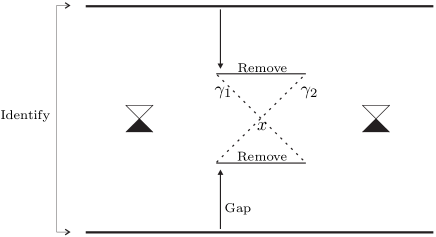
Figure 1: A non-totally vicious non-chronological spacetime obtained from Minkowski spacetime by removing two spacelike segments and by identifying two lines as displayed. If the gap is large enough there is only one component of the chronology violating set and no lightlike line though $\gamma_{1}$ and $\gamma_{2}$ are inextendible lightlike geodesics. If the gap is small enough there are two components, the interxection of their boundaries being the event $x$. The curves $\gamma_{1}$ and $\gamma_{2}$ are in this case lightlike lines as expected from theorem 4.5

Theorem 4.4.

Let $\gamma_{1}:\mathbb{R}\to M$ and $\gamma_{2}:\mathbb{R}\to M$ be two distinct lightlike lines which intersect at a event $x$, and assume that neither $\gamma_{1}$ nor $\gamma_{2}$ intersect the closure of the chronology violating set, then strong causality holds at every point of $\gamma_{1}$ and $\gamma_{2}$.

Proof.

Without loss of generality assume $\gamma_{1}(0)=\gamma_{2}(0)=x$. By theorem 4.3 either strong causality is satisfied at $x$ and hence it is satisfied at every point of $\gamma_{1}$ and $\gamma_{2}$ or it is not satisfied at $x$ and hence it fails at every point of $\gamma_{1}$ and $\gamma_{2}$ (case (ii3) of theorem 4.3 can not hold in this case otherwise $x$ would belong to the closure of the chronology violating set). In the latter case, split $\gamma_{1}$ in two parts $\gamma_{1}^{+}:[0,+\infty)\to M$, and $\gamma_{1}^{-}:(-\infty,0]\to M$ and do the same with $\gamma_{2}$. By the same theorem for every $\epsilon>0$, defined $x_{1}^{+}=\gamma_{1}(\epsilon)$, $x_{1}^{-}=\gamma_{1}(-\epsilon)$, $x_{2}^{+}=\gamma_{2}(\epsilon)$, $x_{2}^{-}=\gamma_{2}(-\epsilon)$, it is $(x_{2}^{+},x_{2}^{-})\in\bar{J}^{+}$.

Since the lines are distinct it is possible to round the corner at $x$ of $\gamma^{+}_{2}\circ\gamma_{1}^{-}$, and it is possible to do the same for $\gamma^{+}_{1}\circ\gamma_{2}^{-}$. As a result, $(x_{1}^{-},x_{2}^{+})\in I^{+}$ and $(x_{2}^{-},x_{1}^{+})\in I^{+}$, and using the fact that $I^{+}$ is open it follows that $(x_{1}^{-},x_{1}^{+})\in I^{+}$, a contradiction since $\gamma_{1}$ is a line. ∎

Clearly, the previous theorem holds even if the the lightlike lines are replaced with lightlike maximizing segments which intersect at a event which corresponds to parameter values which stay in the interior of their respective domains.

It is well known since the work of Brandon Carter that the chronology violating set is the union of open components, where two points $p$ and $q$ belong to the same component whenever $p\ll q\ll p$. In some cases the boundaries of the components may intersect (see figure 1).

Theorem 4.5.

Let $B_{1}=\dot{C}_{1}$ and $B_{2}=\dot{C}_{2}$ where $C_{1}$ and $C_{2}$ are distinct components of the chronology violating set of $(M,g)$. Through every point of $B_{1}\cap B_{2}$ (which may be empty) there passes a lightlike line entirely contained in $B_{1}\cup B_{2}$. In particular a spacetime without lightlike lines has a chronology violating set with components having disjoint closures.

Proof.

Assume that $x\in B_{1}\cap B_{2}$, and let $\gamma^{(1)}_{n}$ be a sequence of closed timelike curves of starting point and ending point $x^{(1)}_{n}$, $x^{(1)}_{n}\in C_{1}$ and $x^{(1)}_{n}\to x$ (thus $\gamma^{(1)}_{n}$ are contained in $C_{1}$). Analogously, let $\gamma^{(2)}_{n}$ be a sequence of closed timelike curves of starting point and ending point $x^{(2)}_{n}$, $x^{(2)}_{n}\in C_{2}$ and $x^{(2)}_{n}\to x$ (thus $\gamma^{(2)}_{n}$ are contained in $C_{2}$). Apply the limit curve theorem case (2) to $\gamma^{(1)}_{n}$ with $z=x$. If $b<+\infty$ then $\gamma^{(1)x}$ is a closed causal curve, it must be achronal since if $p,q\in\gamma^{(1)x}$, $p\ll q$, then $x\leq p\ll q\leq x$ and hence $x\ll x$ which implies $x\in C_{1}$ a contradiction. Thus $\gamma^{(1)x}$ is a geodesic with no discontinuity in the tangent vectors at $x$. It can be extended to a lightlike line $\gamma$ by making infinite rounds over $\gamma^{(1)x}$. Moreover, note that $\gamma^{(1)x}$ can’t have any point $p$ in $C_{1}$ otherwise $x\leq p\ll p\leq x$ and again $x\ll x$, $x\in C_{1}$, a contradiction, thus $\gamma\subset\dot{C}_{1}$.

It remains to consider the case in which the limit curve theorem case (2) applies to $\gamma^{(1)}_{n}$ and $\gamma^{(2)}_{n}$ with $b=+\infty$. With the notations of the limit curve theorem, there are future inextendible continuous causal curves $\gamma^{(1)x}\subset\bar{C}_{1}$, $\gamma^{(2)x}\subset\bar{C}_{2}$ and past inextendible continuous causal curves $\gamma^{(1)z}\subset\bar{C}_{1}$, $\gamma^{(2)z}\subset\bar{C}_{2}$. Assume that neither $\gamma^{(21)}=\gamma^{(1)x}\circ\gamma^{(2)z}$ nor $\gamma^{(12)}=\gamma^{(2)x}\circ\gamma^{(1)z}$ are lightlike lines. There are points $\bar{z}^{(2)}\in\gamma^{(2)z}$, $\bar{x}^{(1)}\in\gamma^{(1)x}$, $\bar{z}^{(2)}\ll\bar{x}^{(1)}$, and $\bar{z}^{(1)}\in\gamma^{(1)z}$, $\bar{x}^{(2)}\in\gamma^{(2)x}$, $\bar{z}^{(1)}\ll\bar{x}^{(2)}$. Since $I^{+}$ is open there are open sets $V^{(2)}\ni\bar{z}^{(2)}$, $U^{(1)}\ni\bar{x}^{(1)}$, $V^{(1)}\ni\bar{z}^{(1)}$ and $U^{(2)}\ni\bar{x}^{(2)}$ such that $V^{(2)}\times U^{(1)}\subset I^{+}$, $V^{(1)}\times U^{(2)}\subset I^{+}$. But $(U^{(1)}\cap C_{1})\times(V^{(1)}\cap C_{1})\subset I^{+}$ because any two points of $C_{1}$ are chronologically related. Analogously, $(U^{(2)}\cap C_{2})\times(V^{(2)}\cap C_{2})\subset I^{+}$. These relations prove that it is possible to find two points $p\in C_{1}$ and $q\in C_{2}$ such that $p\ll q\ll p$ and thus the two components would coincide. The contradiction proves that $\gamma^{(21)}$ or $\gamma^{(12)}$ is a lightlike line. Assume it is the former the latter case being analogous. The curve $\gamma^{(1)x}$ can’t intersect $C_{1}$ otherwise taken any two points of $\gamma^{(1)x}$ in $C_{1}$ they would be chronologically related in contradiction with the achronality of $\gamma^{(21)}$. Thus $\gamma^{(1)x}\subset\dot{C}_{1}$ and analogously, $\gamma^{(2)z}\subset\dot{C}_{2}$, in conclusion $\gamma^{(21)}\subset B_{1}\cup B_{2}$. ∎

5 Conclusions

In the first sections of this work the topic of limit curve theorems in Lorentzian geometry has been reviewed. Since the aim was the formulation of a limit curve theorem which holds even in the case of curves with endpoints, the definition of uniform convergence on compact subsets has been generalized to the case in which the converging curves do not have the same domain of definition.

The upper semi-continuity of the length functional has been given a new proof which is suitable to this generalized circumstance (theorem 2.4). It avoids any mention to the property of strong causality while it replaces $C^{0}$ convergence with uniform converge.

The notion of limit maximizing sequence has been generalized to the case of curves without endpoints, as well as the theorem that the uniform limit of a limit maximizing sequence is a maximizing curve (theorem 2.13).

The central result of the work, theorem 3.1, is separated into three parts.

Point (1) gives the generalization of Beem et al. limit curve lemma to the case of curves with endpoints, with a few more observations which are helpful in order to establish whether the limit curve is inextendible or not. Thanks to the fact that it holds for curves with endpoints, it can be used to construct limit maximizing sequences where one or both endpoints go to infinity. Thus it is useful in order to establish the existence of lines or rays passing through a point.

Point (2) focuses on the case in which there have been given, since the beginning, two limit events $x$ and $z$ and not only one as in (1). This case is very useful in applications, especially when it comes to prove the connectedness of spacetime through maximizing geodesics or similar results. It also becomes specially interesting when $x$ and $z$ coincide. In this case it provides information on the existence of lightlike lines given suitable causality violations on the spacetime. I will consider these aspects in a related work . If the sequence of curves is limit maximizing, point (2) gives a bound to the sum of the lengths of the two limit curves, generalizing a key observation by Newman [13].

Point (3) focuses on a very general case in which the limit points given in the beginning can be infinite but numerable. In this case it is proved that through each one of them there passes a uniform limit curve and in case of a limit maximizing sequence, an upper bound to the sum of their lengths has been given.

Some consequences of the limit curve theorem have been considered in the last sections. It has been proved for instance that in chronological spacetimes the maximizing lightlike segments defined over open intervals are such that strong causality either is everywhere violated or everywhere verified over the curve (theorem 4.3). A consequence is that if in a chronological spacetime two distinct lightlike lines intersect each other then strong causality holds at the points of their union (theorem 4.4).

Finally, the last result has been the proof that any spacetime without lightlike lines has a chronology violating set such that the closures of its components are disjoint.

References

- [1] E. Aguirre-Dabán and M. Gutiérrez-López. On the topology of stable causality. Gen. Relativ. Gravit., 21:45–59, 1989.
- [2] J. K. Beem. Conformal changes and geodesic completeness. Commun. Math. Phys., 49:179–186, 1976.
- [3] J. K. Beem, P. E. Ehrlich, and K. L. Easley. Global Lorentzian Geometry. Marcel Dekker Inc., New York, 1996.
- [4] H. Busemann. Timelike spaces. Dissertationes Mathematicae (formerly Rozprawy Matematyczne - Instytut Matematyczny Polskiej Akademii Nauk), 53:1–52, 1967.
- [5] G. Buttazzo and M. Giaquinta. One-dimensional variational problems. Oxford University Press, Oxford, 1998.
- [6] J.-H. Eschenburg and G. J. Galloway. Lines in space-times. Comm. Math. Phys., 148:209–216, 1992.
- [7] G. J. Galloway. Curvature, causality and completeness in space-times with causally complete spacelike slices. Math. Proc. Camb. Phil. Soc., 99:367–375, 1986.
- [8] S. W. Hawking and G. F. R. Ellis. The Large Scale Structure of Space-Time. Cambridge University Press, Cambridge, 1973.
- [9] E. Minguzzi. The causal ladder and the strength of -causality. I. Class. Quantum Grav., 25:015009, 2008.
- [10] E. Minguzzi. The causal ladder and the strength of -causality. II. Class. Quantum Grav., 25:015010, 2008.
- [11] E. Minguzzi. Non-imprisonment conditions on spacetime. J. Math. Phys., 49:062503, 2008.
- [12] E. Minguzzi and M. Sánchez. The causal hierarchy of spacetimes, volume H. Baum, D. Alekseevsky (eds.), Recent developments in pseudo-Riemannian geometry, of ESI Lect. Math. Phys., pages 299 – 358. Eur. Math. Soc. Publ. House, Zurich, 2008. gr-qc/0609119.
- [13] R. P. A. C. Newman. A proof of the splitting conjecture of S.-T. Yau. J. Diff. Geom., 31:163 –184, 1990.
- [14] B. O’Neill. Semi-Riemannian Geometry. Academic Press, San Diego, 1983.
- [15] R. Penrose. Techniques of Differential Topology in Relativity. Cbms-Nsf Regional Conference Series in Applied Mathematics. SIAM, Philadelphia, 1972.
- [16] H. Seifert. The causal boundary of space-times. Gen. Relativ. Gravit., 1:247–259, 1971.