Aharonov-Bohm ring with a side-coupled atomic cluster: magneto-transport and the selective switching effect

Abstract

Abstract

We report electronic transmission properties of a simple tight binding Aharonov-Bohm ring threaded by a magnetic flux, to one arm of which a finite cluster of atoms has been attached from one side. We demonstrate that, by suitably choosing the number of scatterers in each arm of the quantum ring, the transmission across the ring can be completely blocked when the ring is decoupled from the atomic cluster and the flux threading the ring becomes equal to half the fundamental flux quantum. A novel transmission resonance then occurs immediately as the coupling between the ring and the impurity cluster is switched ‘on’. It is shown that the delta-like transmission resonances occur precisely at the eigenvalues of the side coupled chain of atoms. The ‘switching’ effect can be observed either for all the eigenvalues of the isolated atomic cluster, or for a selected set of them, depending on the number of scatterers in the arms of the ring. The ring-dot coupling can be gradually increased to suppress the oscillations in the magneto-transmission completely. However, the suppression can lead either to a complete transparency or no transmission at all, occasionally accompanied by a reversal of phase at special values of the magnetic flux.

I Introduction

Simple tight binding models of mesoscopic systems have been quite extensively studied in recent times kub02 -xiong06 with a view to understand the basic features of electronic transport in quantum dots (QD) or the magneto-transport in closed loop geometries such as an Aharonov-Bohm (AB) ring. One reason behind such model studies is definitely the simple geometry of the models which enables one to derive exact results and to look into the possible causes of certain salient features observed in the transport properties of real life small scale semiconducting or metallic systems. The other reason can be attributed to the immense success of nano-technology and the use of precision instruments such as a scanning tunnel microscope (STM) which can be used to build low dimensional nanostructures with tailor-made geometries. One such geometry, which will be our concern in this communication, is an AB ring threaded by a magnetic flux $\Phi$ and with a finite segment of $N$ atomic sites attached to one arm of the ring at an arbitrary point.

The central feature of electron transport across an AB ring is the periodic oscillation in the magnetoconductance whenever the phase coherence length exceeds the dimension of the sample ab59 . Büttiker et al butt83 provided an early formulation of the problem. The transport in such a closed geometry was re-addressed by Gefen et al gefen84 who obtained an exact expression for the two-terminal conductance across the ring. Using a discrete tight binding formulation the two-terminal conductance was also examined by D’Amato et al amato89 , and subsequently, by Aldea et al aldea92 . A non-trivial change in the transport of an AB ring is observed when the ring contains a quantum dot (QD) either embedded in an arm, or side coupled to it yacob95 -holl01 . Motivated by the experiment of Yacoby et al yacob95 , Yeyati and Büttiker levy95 prescribed an exact formulation of the magnetoconductance of an AB ring with a QD embedded in its arm. A similar problem with a multi-terminal geometry was later addressed by Kang kang99 . The QD-AB ring hybrid system also received attention in relatively recent experiments by Meier et al meier04 and Kobayashi et al koba02 -koba04 with a focus on the study of single electron charging and suppression of AB oscillations meier04 , and the Fano resonance in the magnetoconductance koba02 -koba04 .

In a quantum dot discrete energy levels arise as a consequence of confinement of electrons in all three directions. This has inspired a considerable number of theoretical works involving a discrete lattice of the so called ‘single level’ QD’s kub02 , mimicked by ‘atomic’ sites arranged either in an open geometrical arrangement or in a closed AB ring within a tight binding formalism. For example, QD’s, single, or in an array, side coupled to an open chain have already received attention in the context of Kondo effect torio02 , one electron transport ore03 , rod03 , adam04 and Dicke effect paore04 . The prospect of engineering Fano resonances mir05 -kiv05 , design of spin filters lee06 and the localization-delocalization problem pou02 in a series of atomic clusters side coupled to an infinite lattice have also been discussed in details.

Motivated by such simple models which, inspite of their simplicity, brings out the rich quantum coherence effects exhibited by a mesoscopic system, we re-visit the problem of magneto-transport in an AB ring threaded by a magnetic flux, but now with a chain of $N$ atomic sites (an array of single level QD’s) attached to one arm of the ring. Inspite of the previous studies we believe that the interplay of the closed loop geometry and the eigenvalue spectrum of the dangling QD array is little studied and, is likely to provide new features in the electronic transport, that might throw some light on the potential of such systems as novel quantum devices. This is our main objective.

We focus on the role of the ring-dot coupling in particular, and come across several interesting results. For example, it is found that the ring-dot system displays a ‘switching’ action for small values of the ring-dot coupling at selected energies of the electron when the flux penetrating the ring is $\Phi=\Phi_{0}/2$. The energy values (at which the switching takes place), for a given size of the QD array coupled to the ring, belong to the set of eigenvalues of the isolated QD array, and depend on the number of scatterers in the upper and the lower arms of the ring. A gradual increase in the ring-dot coupling suppresses the AB oscillations and is accompanied by occasional transmission phase-reversals at specific values of the magnetic flux.

In what follows, we present the model and the method in section II. Section III contains the results and the related discussion and we draw conclusion in section IV.

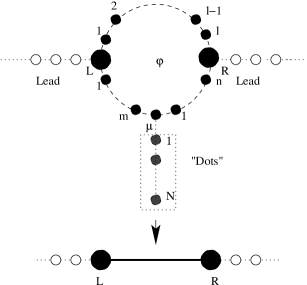
Figure 1: The quantum ring and the side coupled chain of quantum dots. The sites $L$ and $R$ (bigger solid circles) mark the left and the right junctions with the leads, and the site marked $\mu=+1$ is the ‘connecting’ point of the side coupled FA chain.

II The model and the method

We begin by referring to Fig.1. The ring contains $l$ atoms in the upper arm, excluding the sites marked $L$ and $R$ where the leads join the ring. The site marked $\mu$ in the lower arm is the point where the dangling QD chain is attached. There are $m$ sites to the left of $\mu$ and $n$ sites to its right. Changing $m$ and $n$ therefore shifts the location of the attachment of the ‘defect’ chain. The Hamiltonian of the lead-ring-dot-lead system, in the standard tight binding form, is written as,

$$H=H_{lead}+H_{ring}+H_{dot}+H_{ring-dot}+H_{ring-lead}$$ (1)

where,

$$H_{lead} = \epsilon_{0}\sum_{i=-\infty}^{L-1}c_{i}^{{\dagger}}c_{i}+\epsilon_{0}\sum_{i=R+1}^{\infty}c_{i}^{{\dagger}}c_{i}+t_{0}\sum_{<ij>}c_{i}^{{\dagger}}c_{j}$$

$$H_{ring} = \epsilon_{L}r_{L}^{{\dagger}}r_{L}+\epsilon_{R}r_{R}^{{\dagger}}r_{R}+t_{0}\exp(i\gamma)\sum_{<ij>}r_{i}^{{\dagger}}r_{j}+h.c.$$

$$H_{dot} = \sum_{i=1}^{N}\epsilon_{i}d_{i}^{{\dagger}}d_{i}+t_{0}\sum_{i=1}^{N-1}d_{i}^{{\dagger}}d_{j}+h.c.$$

$$H_{ring-dot} = \lambda(r_{\mu}^{{\dagger}}d_{1}+h.c.)$$

$$H_{ring-lead} = t_{0}(r_{L}^{{\dagger}}c_{L-1}+r_{R}^{{\dagger}}c_{R+1})$$ (2)

In the above, $c^{{\dagger}}(c)$, $r^{{\dagger}}(r)$, and $d^{{\dagger}}(d)$ represent the creation (annihilation) operators for the leads, the ring and the QD chain respectively. $r_{L}$$(r_{L}^{\dagger})$ and $r_{R}(r_{R}^{\dagger})$ represent the same at the lead-ring connecting sites $L$ and $R$ respectively. The on-site potential at the leads, in the QD chain and in the bulk of the ring is taken to be $\epsilon_{0}$ for every site including the site marked $\mu$. The lead-ring connecting sites have been assigned the on-site potentials $\epsilon_{L}$ and $\epsilon_{R}$ respectively. The amplitude of the hopping integral is taken to be $t_{0}$ throughout except the hopping from the site $\mu$ in the ring to the first site of the QD chain, which has been symbolized as $\lambda$ and represents the ‘strength’ of coupling between the ring and the QD array. $\gamma$ is given by $\gamma=2\pi\Phi/(l+m+n+1)\Phi_{0}$, where, $\Phi$ is the flux threading the ring and $\Phi_{0}=hc/e$ is the fundamental flux quantum. The task of solving the Schrödinger equation to obtain the stationary states of the system can be reduced to an equivalent problem of solving a set of the following difference equations:

For the sites $L$ and $R$ at the ring-lead junctions,

$$(E-\epsilon_{L})\psi_{L} = t_{0}e^{i\gamma}\psi_{1,\cal U}+t_{0}e^{-i\gamma}\psi_{1,\cal L}+t_{0}\psi_{L-1}$$

$$(E-\epsilon_{R})\psi_{R} = t_{0}e^{-i\gamma}\psi_{l,\cal U}+t_{0}e^{i\gamma}\psi_{m+n+1,\cal L}+t_{0}\psi_{R+1}$$

In the above, $\psi_{L-1}$ and $\psi_{R+1}$ represent the amplitudes of the wave function at the sites on the lead which are closest to the points $L$ and $R$, and, $\cal U$ and $\cal L$ in the subscripts refer to the ‘upper’ and the ‘lower’ arms respectively.

For the sites in the bulk of the ring the equations are,

$$(E-\epsilon_{0})\psi_{j,\cal U} = t_{0}e^{-i\gamma}\psi_{j-1,\cal U}+t_{0}e^{i\gamma}\psi_{j+1,\cal U}$$

$$(E-\epsilon_{0})\psi_{j,\cal L} = t_{0}e^{i\gamma}\psi_{j-1,\cal L}+t_{0}e^{-i\gamma}\psi_{j+1,\cal L}$$ (4)

where, by $j+1$ and $j-1$th we symbolize the sites to the right and to the left of the $j$th site in any arm of the ring.

For the site marked $\mu$ in the lower arm of the ring, the equation is,

$$(E-\epsilon_{0})\psi_{\mu,\cal L}=t_{0}e^{i\gamma}\psi_{\mu-1,\cal L}+t_{0}e^{-i\gamma}\psi_{\mu+1,\cal L}$$ (5)

$\mu\pm 1$ implying the sites to the right and to the left of the site marked $\mu$ respectively. Finally, for the QD array we have the following set of difference equations,

$$(E-\epsilon_{1})\psi_{1} = \lambda\psi_{\mu}+t_{0}\psi_{2}$$

$$(E-\epsilon_{j})\psi_{j} = t_{0}\psi_{j-1}+t_{0}\psi_{j+1}$$

$$(E-\epsilon_{N})\psi_{N} = t_{0}\psi_{N-1}$$ (6)

where the central set of equations above refer to the bulk sites viz. $j=2,...N-1$ in the QD array.

The process of calculating the transmission coefficient across such a ring-dot system consists of the following steps. First, the dangling QD chain is ‘wrapped’ into an effective site by decimating the amplitudes $\psi_{2}$ to $\psi_{N}$ from Eq.(6). The renormalized on-site potential of the first site of the QD array is given by arun07 ,

$$\tilde{\epsilon}=\epsilon_{0}+\frac{t_{0}U_{N-3}(x)}{U_{N-2}(x)}+\frac{t_{0}^{2}}{U_{N-2}^{2}(x)}\frac{1}{E-\epsilon_{0}-\frac{t_{0}U_{N-3}(x)}{U_{N-2}(x)}}$$ (7)

for $N\geq 2$. For $N=1$, we simply have $\tilde{\epsilon}=\epsilon_{0}+\lambda^{2}/(E-\epsilon_{0})$. Here, $x=(E-\epsilon_{0})/2t_{0}$ and $U_{N}(x)$ is the $N$th order Chebyshev polynomial of the second kind, with $U_{0}=1$ and $U_{-1}=0$ grim00 . This ‘effective’ site is coupled to the site marked $\mu$ in the lower arm of the ring via a hopping integral $\lambda$. In the second step, the effective site with on-site potential is further ‘folded’ back into the site $\mu$, whose renormalized on-site potential now reads arun07 ,

$$\epsilon^{*}=\epsilon_{0}+\frac{\lambda^{2}}{E-\tilde{\epsilon}}.$$ (8)

We now have a ring with $l$ atoms in the upper arm and an effective site at position $\mu$ in the lower arm, flanked by $m$ atoms on its left and $n$ atoms on the right, so that there is a total of $m+n+1$ atoms in the lower arm. This is just the case of a QD with an energy dependent on-site potential embedded in an arm of an AB-ring. In the final step, all the $l+m+n+1$ atoms are decimated using the set of appropriate difference equations (3) and (4), to reduce the ring into an effective diatomic molecule (Fig.1). The renormalized values of the on-site potential at the two extremeties of the molecule are given by,

$$\tilde{\epsilon}_{L} = \epsilon_{0}+t_{0}\left(\frac{U_{l-1}}{U_{l}}+\frac{U_{m-1}}{U_{m}}\right)+\frac{t_{0}^{2}}{U_{m}^{2}}F(E,\lambda,m,n)$$

$$\tilde{\epsilon}_{R} = \epsilon_{0}+t_{0}\left(\frac{U_{l-1}}{U_{l}}+\frac{U_{n-1}}{U_{n}}\right)+\frac{t_{0}^{2}}{U_{n}^{2}}F(E,\lambda,m,n)$$

where, for a fixed set of $\epsilon_{0}$ and $t_{0}$,

$$F(E,\lambda,m,n)=\left[E-\epsilon^{*}-t_{0}\left(\frac{U_{m-1}}{U_{m}}+\frac{U_{n-1}}{U_{n}}\right)\right]^{-1}$$ (10)

The time reversal symmetry of the hopping integral between the atoms at $L$ and $R$ of the diatomic molecule is broken due to the flux threading the ring, and is given by,

$$t_{F}=\frac{t_{0}}{U_{l}}e^{i(l+1)\gamma}+\frac{t_{0}^{2}}{U_{m}U_{n}}F(E,\lambda,m,n)e^{-i(m+n+2)\gamma}$$ (11)

for the forward hopping from $L$ to $R$ and by $t_{B}=t_{F}^{*}$ for the backward hopping from $R$ to $L$. The transmission coefficient across the effective diatomic molecule is given by stone81 ,

$$T=\frac{4\sin^{2}qa}{|M_{12}-M_{21}+(M_{11}-M_{22})\cos qa|^{2}+|M_{11}+M_{22}|^{2}\sin^{2}qa}$$ (12)

where, $a$ is the lattice constant in the leads, taken to be equal to one throughout the calculation. In what follws, we discuss various aspects of the electronic transmission across the ring-QD array system. We fix the on-site potential at all sites, including the QD chain, as $\epsilon_{0}$ and the hopping integrals has been kept equal to $t_{0}$ throughout, except the ring-QD array coupling $\lambda$. The ‘defect’ that we hang from an otherwise perfect ring is thus only of a topological nature.

III Results and Discussions

III.1 Suprression of AB oscillations

Figure 2: The gradual suppression of AB oscillations in the transmission spectrum as the ring-dot coupling increases. (a) $E=10^{-6}$, $l=13$, $m=n=6$ and $N=5$. Here, $\lambda=0.001$ (solid), $0.002$ (dashed), $0.005$ (dotted) and $0.1$ (dot-dash). (b) $E=10^{-6}$, $L=7$, $m=3$, $n=8$ and $N=7$. $\lambda=0.001$ (solid), $0.004$ (dashed), $0.005$ (dotted) and $0.006$ (dot-dash). (c) $E=0.618011988$, $l=9$, $m=3$, $n=8$ and $N=4$. The values of $\lambda$ are, $0.001$ (solid), $0.007$ (dashed), $0.01$ (dotted) and $0.5$ (dot-dash) respectively. Other parameters are, $\epsilon_{0}=0$, $t_{0}=1$ and the energy and $\lambda$ are measured in unit of $t_{0}$, and the flux is measured in unit of $\Phi_{0}$

In all transmission profiles the ring-dot coupling $\lambda$ plays a crucial role. The first effect that we present is a supression of the AB oscillations as a function of $\lambda$. We choose the energy $E$ from a specially selected set obtained by solving the equation $E-\tilde{\epsilon}=0$. For these $E$-values the suppression of the AB oscillations can be directly worked out from our formulation. It is to be appreciated that the eigenvalues of the isolated quantum dot array are obtained by solving the polynomial equation $E-\tilde{\epsilon}=0$ mir05 -arun07 . We select any one of the roots, name it $\tilde{\epsilon}_{0}$, and fix $\lambda\neq 0$. This last condition is important.

A close look at the expression of $\epsilon^{*}$ reveals that for $E=\tilde{\epsilon}_{0}$ (in fact, for any real root of the equation $E-\tilde{\epsilon}=0$) we get $\epsilon^{*}=\infty$. This leads to the following reduced forms of $\epsilon_{L}$, $\epsilon_{R}$ and $t_{F}(=t_{B}^{*})$:

$$\tilde{\epsilon}_{L} = \epsilon_{0}+t_{0}\left(\frac{U_{l-1}}{U_{l}}+\frac{U_{m-1}}{U_{m}}\right)$$

$$\tilde{\epsilon}_{R} = \epsilon_{0}+t_{0}\left(\frac{U_{l-1}}{U_{l}}+\frac{U_{n-1}}{U_{n}}\right)$$

$$t_{F} = \frac{t_{0}}{U_{l}}e^{i(l+1)\gamma}$$ (13)

We observe that the ring-dot coupling $\lambda$ does not appear in any of these expressions. This is because of the selection $E=\tilde{\epsilon}_{0}$ and a non-zero $\lambda$, however small. Let us now define, $\cos(qa)=(E-\epsilon_{0})/2t_{0}=(\tilde{\epsilon}_{0}-\epsilon_{0})/2t_{0}=\delta/2t_{0}$, $\tilde{\epsilon}_{0}-\tilde{\epsilon}_{L}=\xi_{1}$ and $\tilde{\epsilon}_{0}-\tilde{\epsilon}_{R}=\xi_{2}$. With these, the transfer matrix elements for the diatomic molecule read,

$$M_{11} = \left[\frac{\xi_{1}\xi_{2}U_{l}}{t_{0}^{2}}-\frac{1}{U_{l}}\right]e^{-i(l+1)\gamma}$$

$$M_{12} = -\frac{\xi_{2}U_{l}}{t_{0}}e^{-i(l+1)\gamma}$$

$$M_{21} = \frac{\xi_{1}U_{l}}{t_{0}}e^{-i(l+1)\gamma}$$

$$M_{22} = -U_{l}e^{-i(l+1)\gamma}$$ (14)

Finally, the transmission coefficient is given by,

$$T=\frac{4[1-\frac{\delta^{2}}{4t_{0}^{2}}]}{|d_{1}|^{2}+|d_{2}|^{2}}$$ (15)

where,

$$d_{1} = \frac{e^{-i(l+1)\gamma}}{t_{0}}\left[\left(\frac{\xi_{1}\xi_{2}U_{l}}{t_{0}^{2}}+\frac{U_{l}^{2}-1}{U_{l}}\right)\frac{\delta}{2}-(\xi_{1}+\xi_{2})U_{l}\right]$$

$$d_{2} = e^{-i(l+1)\gamma}\left(\frac{\xi_{1}\xi_{2}U_{l}}{t_{0}^{2}}-\frac{U_{l}^{2}+1}{U_{l}}\right)\sqrt{1-\frac{\delta^{2}}{4t_{0}^{2}}}$$ (16)

As we observe, $|d_{1}|^{2}$ and $|d_{2}|^{2}$ and hence $T$, are independent of the flux. That is, the AB-oscillations are suppressed whenever the Fermi energy coincides with any of the discrete eigenvalues of the isolated QD-array.

In view of the above calculation, a few pertinent observations should be given due importance. Let us detune $E$ slightly from an eigenvalue of the QD-array. That is, let’s set $E-\tilde{\epsilon}_{0}=\Delta$, $\Delta$ being very small. How does the shape of the AB-oscillation get altered in the neighborhood of $E=\tilde{\epsilon}_{0}$ ? In this case we have,

$$\epsilon^{*}=\epsilon_{0}+\frac{\lambda^{2}}{\Delta}$$ (17)

Clearly, if $\lambda\neq 0$, but very very small so that $\lambda^{2}\sim{\cal O}(\Delta)$, then the analysis as given above, is not valid, as $\epsilon^{*}$ is not infinity any more. As a result, we shall observe AB-oscillations in the transmission spectrum in general. If we gradually increase the value of $\lambda$ so that $\Delta\ll\lambda$, or even smaller, then we essentially keep on making $\lambda^{2}/\Delta$ and hence $\epsilon^{*}$ larger and larger. This results in the gradual suppression of the amplitude of the AB-oscillations, and finally, when $\lambda^{2}/\Delta$ becomes a very large number (dictated by the machine precision), the transmission coefficient ($T$) becomes independent of the flux threading the ring. AB-oscillations disappear completely.

An interesting feature of the AB oscillations in such cases is that, a gradual increase in the value of $\lambda$ can lead either to $T=1$ (Fig.2a) or to $T=0$ (Figs.2b and 2c). This depends on the combination of the size of the ring (i.e. on $l$, $m$ and $n$) and the length of the QD array ($N$). In every case however, the progress towards $T=1$ or $T=0$ is accompanied by a gradual suppression of the AB oscillations. Most interestingly, for a set of values of $l$, $m$, $n$ and $N$, the phase of the AB oscillations is reversed at specific values of the magnetic flux as soon as $\lambda$ exceeds some ‘critical’ value. Incidentally, a similar observation in a simpler geometry was reported by Kubala and König as well kub02 . The present cases are depicted in Fig.$2$(b) and $2$(c) where the reversal is observed at $\Phi=\Phi_{0}/2$ and $3\Phi_{0}/2$ (odd multiple of $\Phi_{0}/2$ in general). However, with different combinations of $l$, $m$, $n$ and $N$, the reversal can take place at other flux values as well, for example at $\Phi=0$ and $\Phi=\Phi_{0}$. We have not been able to obtain exact criterion for the phase reversal. However, extensive numerical search has revealed that this is true for various combinations of the size of the ring and the length of the QD array.

Before ending, it should be mentioned that, the flux indepence that we have discussed above, is basically caused by the divergence of $\epsilon^{*}$ at special energies. This divergence can also be achieved for any arbitrary energy other that the eigenvalues of the isolated QD array, by letting $\lambda\rightarrow\infty$. Such a situation, as we have carefully observed, but do not report here to save space, leads to a flux independent $T-E$ spectrum.

III.2 Selective switching

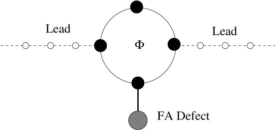
Figure 3: A simple $4$-site ring with a single FA defect attached to it

At first, we note that, for $l=m+n+1$, i.e., for an equal number ($l$) atoms in the two arms, and with $\lambda=0$, the $L-R$ hopping integral in the effective diatomic molecule is real, and reads,

$$t_{F}=\frac{2t_{0}}{U_{l}}\cos(\frac{\pi\Phi}{\Phi_{0}})$$ (18)

$t_{B}$ is of course, equal to $t_{F}$. It is now clear that for $\Phi=\Phi_{0}/2$, the effective hopping integral becomes zero, resulting in $T=0$ (an antiresonance) independent of the energy of the electron. As soon as the ring-dot coupling $\lambda$ assumes a non-zero value, interesting transmission behavior is observed. To get a clearer understanding, we refer to Fig.3, which is a ring with just one atom in both the lower and the upper arms with a single QD with an on-site potential $\epsilon_{D}$ coupled to the atom in the lower arm. This is a simple modification of the model used by Kubala and König kub02 . For this simple geometry, with $\lambda\neq 0$, we get,

$$\tilde{\epsilon}_{L} = \epsilon_{0}+\frac{t_{0}^{2}}{E-\epsilon_{0}}+\frac{t_{0}^{2}(E-\epsilon_{D})}{(E-\epsilon_{0})(E-\epsilon_{D})-\lambda^{2}}$$

$$t_{F} = (-i)t_{0}^{2}\frac{\lambda^{2}}{(E-\epsilon_{0})[(E-\epsilon_{0})(E-\epsilon_{D})-\lambda^{2}]}$$ (19)

with $\tilde{\epsilon}_{R}=\tilde{\epsilon}_{L}$ and $t_{B}=t_{F}^{*}$. Using these, one can work out the transfer matrix elements for the diatomic molecule, in the limit $E\rightarrow\epsilon_{D}$, to be equal to,

$$\lim_{E\rightarrow\epsilon_{D}}M_{11} = \frac{-i\delta(2t_{0}^{2}-\delta^{2})}{t_{0}^{3}}$$

$$\lim_{E\rightarrow\epsilon_{D}}M_{12} = \frac{-i(t_{0}^{2}-\delta^{2})}{t_{0}^{2}}$$

$$\lim_{E\rightarrow\epsilon_{D}}M_{21} = \frac{i\delta(2t_{0}^{2}-\delta^{2})}{t_{0}^{3}}$$

$$\lim_{E\rightarrow\epsilon_{D}}M_{22} = \frac{-i\delta}{t_{0}}$$ (20)

where, $\delta=\epsilon_{0}-\epsilon_{D}$. Inserting these values in the formula for the transmission coefficient, it is observed that $T=1$ for $E=\epsilon_{D}$ with any $\lambda\neq 0$. That is, the presence of a finite ring-dot coupling, however small, triggers ballistic transmission across the ring.

With an arbitrary number of scatteres in either arm of the ring, and the QD array extending beyond one atom, the situation is non-trivial and closed form expressions look extremely cumbersome to deal with. We have conducted extensive and careful numerical investigation to examine several cases. Here, details of a specific case are given which reflect the generic features of the selective switching effect that we wish to highlight.

We choose a situation where the QD array contains, for example, five atoms ($N=5$). The on-site potential $\epsilon_{0}$ and the hopping integral $t_{0}$ are set equal to zero and unity everywhere, including the QD array. We set the magnetic flux $\Phi=\Phi_{0}/2$, and select $l=2m+1$ and $m=n$. The $5$-site QD chain is now diagonalized to get the eigenvalues $0$, $\pm 1$ and $\pm\sqrt{3}$. With $\lambda$ set equal to zero, as discussed before, we get $T=0$ irrespective of energy $E$. Interestingly, it is found that, by choosing a small non-zero value of $\lambda$ and an appropriate set of values for $l$, $m$ and $n$, but always satisfying the requirement $l=2m+1$ and $m=n$, it is possible to make the ring-dot system completely transparent to an incoming electron when its energy becomes equal to some or all of the eigenvalues of the $5$-site QD array. The transmission at any energy outside the set of five eigenvalues mentioned above can be completely suppressed if $\lambda$ is kept small enough. However, a gradual increase in the value of $\lambda$ gives rise to secondary transmission peaks as the ring ‘interacts’ with the QD more strongly. These secondary peaks finally settle into bands of transmission separated by transmission dips, as a result of quantum interference. The important thing to appreciate is that whether we observe complete transparency at a subset of the eigenvalues or for all of them, depends strongly on the mutual tuning of the values of the ring-dot coupling $\lambda$ and $l$, $m$ and $n$. Fig.4 displays the slective switching action when the QD array contains $3$ and $5$ sites respectively (Fig.4a and 4b). In Fig.4a, setting $\lambda=0.08$ and attaching the array to an $(l,m,n)=(1,0,0)$ ring (like one shown in Fig.2), we see that the transmission coefficient is unity (or very close to it) only when energy $E$ is equal to the three eigenvalues of the isolated $3$-dot array, viz, at $E=0$ and $\pm\sqrt{2}$. On the other hand, with $N=5$ (Fig.4b), with $l=17$, $m=n=8$ and $\lambda=0.04$, transmission is triggered only at three of the five eigenvalues. The scenario of course changes as the parameters are varied, keeping $\lambda$ small. However, the ‘smallness’ of $\lambda$ is to be selected by trial method, at least so far as we have checked. In Table 1, we provide a list of such selective values for which $T=1$ (or very close to it) at $\Phi=\Phi_{0}/2$.

Figure 4: Selective switching effect at $\Phi=\Phi_{0}/2$ for a QD array of $3$ sites (a), and $5$ sites (b). In $4(a)$, we have taken $l=1$, $m=n=0$ and $\lambda=0.08$. Three transmission peaks at three distinct eigenvalues $E=0$ and $\pm\sqrt{2}$ of the isolated $3$-site QD chain are visible. In (b) $l=17$, $m=n=8$, $N=5$ and $\lambda=0.04$. Peaks appear at $E=0,\pm\sqrt{3}$, and transmission at two other eigenvalues of the isolated QD chain, viz, at $E=\pm 1$ are blocked.

(l,m,n)	Typical value of $\lambda$	$T\sim 1$ at $E=$
(12k-1,6k-1,6k-1)	arbitrary	No peak at all
(12k-7,6k-4,6k-4)	0.04	$0$, $\pm\sqrt{3}$
(12k-5,6k-3,6k-3)	0.04-0.045	$\pm 1$, $\pm\sqrt{3}$
(12k+3,6k+1,6k+1)	0.04-0.045	$\pm 1$, $\pm\sqrt{3}$
(12k-11,6k-6,6k-6)	0.05-0.10	$0$, $\pm 1$, $\pm\sqrt{3}$
(12k-3,6k-2,6k-2)	0.05-0.10	$0$, $\pm 1$, $\pm\sqrt{3}$

Table 1. Some typical combinations of $l$, $m$, $n$ and the ring-dot coupling $\lambda$ that give rise to selective swithing at $\Phi=\Phi_{0}/2$. $k$ is a positive integer.

Before we end, it should be noted that the geometry dealt with in the present communication can equivalently be thought as a discrete part (the lower arm plus the QD array) to an infinite linear chain (the left lead plus the upper arm plus the right lead). Considering no magnetic field, we expect Fano lineshapes in the transmission spectrum as a result of an ‘interaction’ of the discrete spectrum of the lower parts with the continuous spectrum offered by the upper section mir05 ,kiv05 . Indeed there are such lineshapes in the transmission resonances, which however get masked due to quantum interference as we take larger and larger size of the ring as well as the QD array.

IV conclusion

We have addressed the issue of transmission across an Aharonov-Bohm ring with a dangling chain of single level quantum dots within a tight binding formalism. In presence of a magnetic flux threading the ring, we discuss the role of the ring-dot coupling in controlling the profile of transmission oscillations. The central feature is a suppression of the AB oscillations with occasional reversal of phase at specific values of the flux. Most interestingly, it is found that, a simultaneous adjustment of the number of scatterers in the arms of the ring and the ring-dot coupling can lead to a complete transparency of the system at some or all of the eigenvalues of the QD array. It is important to note that a bigger ring with large values of $l$, $m$, $n$ (always satisfying the condition $m=n$, $l=2m+1$ and $\Phi=\Phi_{0}/2$) exhibits ballistic transmission $T=1$ for rather low values of the ring-dot coupling $\lambda$. This is because, with a bigger ring the coupled QD array stays far away from the junctions $L$ and $R$. The ‘end effects’ are thus minimised. We have also tested these features with a QD array formed according to the quasiperiodic Fibonacci growth rule arun06 . The essential features like the self-similarity in the electronic transmission are also observed in the selective switching case. Such aspects will be discussed elsewhere.

References

• B. Kubala and J. König, Phys. Rev. B 65, 245301 (2002).
• Z. Y. Zeng, F. Claro, and A. Pérez, phys. Rev. B 65, 085308 (2002).
• M. E. Torio, K. Hallberg, A. H. Cecatto, and C. R. Pretto, Phys. Rev. B 65, 085302 (2002).
• V. Pouthier and G. Girardet, Phys. Rev. B 66, 115322 (2002).
• M. L. Ladrón de Guevara, F. Claro, and P. A. Orellana, Phys. Rev. B 67, 195335 (2003).
• P. A. Orellana, F. Domínuez-Adame, I. Gómez, and M. L. Ladrón de Guevara, Phys. Rev. B 67, 085321 (2003).
• A. Rodríguez, F. Domínguez-Adame, I. Gómez, and P. A. Orellana, Phys. Lett. A 320, 242 (2003).
• Y. -J. Xiong and X. -T. Liang, Phys. Lett. A 330, 307 (2004).
• P. A. Orellana, M. L. Ladrón de Guevara, and F. Claro, Phys. Rev. B 70, 233315 (2004).
• I. Gómez, F. Domínguez-Adame, and P. Orellana, J. Phys.:Condens. Matter 16, 1613 (2004). Phys. Rev. B 70, 035319 (2004).
• M. E. Torio, K. Hallberg, A. E. Miroshnichenko, and M. Titov, Eur. Phys. J. B 37, 399 (2004).
• F. Domínguez-Adame, I. Gómez, P. A. Orellana, and M. L. Ladrón de Guevara, Microelectronics. Jour. 35 87 (2004).
• A. E. Miroshnichenko and Y. S. Kivshar, Phys. Rev. E 72, 056611 (2005).
• A. Chakrabarti, Phys. Rev. B 74, 205315 (2006).
• A. Chakrabarti, Phys. Lett. A 366 507 (2007).
• A. E. Miroshnichenko, S. F. Mingaleev, S. Flach, and Y. S. Kivshar, Phys. Rev. E bf 71, 036626 (2005).
• K. Bao and Y. zheng, Phys. Rev. B 73, 045306 (2005).
• H. Li, T. Lü, and P. Sun, Phys. Lett. A 343, 403 (2005).
• M. Mardaani and K. Esfarjani, Physica E 27, 227 (2005).
• Z.-B. He and Y.-J. Xiong, Phys. Lett. A 349, 276 (2006).
• Y. Aharonov and D. Bohm, Phys. Rev. 115, 485 (1959).
• M. Büttiker, Y. Imry, and R. Landauer, Phys. Lett. A 96, 365 (1983).
• Y. Gefen, Y. Imry, and M. Ya. Azbel, Phys. Rev. Lett. 52, 129 (1984).
• J. L. D’Amatao, H. M. Pastawski, and J. F. Weisz, Phys. Rev. B 39, 3554 (1989).
• A. Aldea, P. Gartner, and I. Corcotoi, Phys. Rev. B 45, 14122 (1992).
• A. Yacoby, M. Heiblum, D. Mahalu, and H. Shtrikman, Phys. Rev. Lett. 74, 4047 (1995).
• R. Schuster, E. Buks, M. Heiblum, D. Mahalu, V. Umansky, and H. Shtrikman, Nature (London) 385, 417 (1997).
• A. W. Holleitner, C. R. Decker, H. Qin, K. Eberl, and R. H. Blick, Phys. Rev. Lett. 87, 256802 (2001).
• A. Levy Yeyati and M. Büttiker, Phys. Rev. B 52, R14360 (1995).
• K. Kang, Phys. Rev. B 59, 4608 (1999).
• L. Meier, A. Fuhrer, T. Ihn, K. Ensslin, W. Wegscheider, and M. Bichler, Phys. Rev. B 69, 241302(R) (2004).
• K. Kobayashi, H. Aikawa, S. Katsumoto, and Y. Iye, Phys. Rev. Lett. 88, 256806 (2002).
• K. Kobayashi, H. Aikawa, A. Sano, S. Katsumoto, and Y. Iye, Phys. Rev. B 70, 035319 (2004).
• M. Lee and C. Bruder, Phys. Rev. B 73, 085315 (2006); R. Wang and J.-Q. Liang, Phys. Rev. B 74, 144302 (2006).
• U. Fano, Phys. Rev. 124, 1866 (1961).
• X. Wang, U. Grimm, and M. Schreiber, Phys. Rev. B 62, 14020 (2000); J. Q. You and Q. B. Yang, J. Phys.:Condens. Matter 2, 2093 (1990).
• A. Douglas Stone, J. D. Joannopoulos, and D. J. Chadi, Phys. Rev. B 24, 5583 (1981).