A comparative study of two phenomenological models of dephasing in series and parallel resistors

Abstract

We compare two phenomenological models of dephasing that are in use recently. We show that the stochastic absorption model leads to reasonable dephasing in series (double barrier) and parallel (ring) quantum resistors in presence and absence of magnetic flux. For large enough dephasing it leads to Ohm’s law. On the other hand a random phase based statistical model that uses averaging over Gaussian random-phases, picked up by the propagators, leads to several inconsistencies. This can be attributed to the failure of this model to dephase interference between complementary electron waves each following time-reversed path of the other.

I Introduction

Dephasing is defined as the process by which quantum mechanical interference is destroyed gradually. An electron in a sample may lose its phase memory via interaction with large number of other degrees of freedom, like a phonon bath or even due to interaction with all other electrons. While the microscopic details of such system-bath interactions leading to dephasing is of interest by itself, we focus on a couple of phenomenological models that are currently in use to understand how dephasing affects many quantum interference phenomena in mesoscopic systems. In a double slit setup, if $\psi_{1}$ and $\psi_{2}$ be the two propagating wave functions that superpose with a phase difference $\phi$, the interference intensity is $A=|\psi_{1}|^{2}+|\psi_{2}|^{2}+2Re[\psi_{1}\psi_{2}\exp(i\phi)]$. In the classical limit of complete decoherence the interference term gets totally suppressed and $A=|\psi_{1}|^{2}+|\psi_{2}|^{2}$.

Most of the mesoscopic samples have dimensions close to the phase coherence length $l_{\phi}$, the length scale over which the electrons lose their phase memory. $l_{\phi}$ can be reduced by increasing temperatureimry . An efficient phenomenological model of dephasing was proposed by BüttikerbuttikerVP ; buttikerVP2 . In this model, one attaches ‘virtual voltage probes’ to a system. The probe absorbs phase coherent electrons and in turn reinjects incoherent electrons back to the system to conserve the overall unitarity of the system plus the probes. This model uses elastic scattering to generate dephasing via introduction of the virtual voltage probe which carries no net current. A series of side coupled self-consistent reservoirs, each drawing zero current, can effectively induce dephasing; moreover this method also allows one to calculate local chemical potentials and temperaturesdib-dabhi . The main drawback in Büttiker’s model is that dephasing occurs locally at the point of contact between the system and voltage probes. However in a natural sample electrons lose phase memory almost uniformly due to interaction with other degrees of freedom.

This can be taken into account by adding a spatially uniform imaginary potential to the Hamiltonianimagpot one can introduce uniform absorption. The main problem with this model is that with increase in imaginary potential one obtains enhanced back reflection, therefore dephasing can not be increased monotonically kumar ; amjIP1 ; amjIP2 . To avoid this, an uniform absorption in the coherent wave function can be introduced via a wave attenuation factorjoshi . This factor reduces the wave amplitude by $\exp(-\alpha\ell)$ after traversal of a length $\ell$ in a free propagating region. Wave attenuation added with a proper incoherent reinjectionbrouwer maintaining the overall unitarity can be used to introduce dephasing in the following way. The three probe Büttiker’s model can be mapped into an effective two terminal geometry by eliminating transmission amplitudes which explicitly depend on the third (virtual) voltage probebrouwer . In the system, a current $I=I_{1}=-I_{2}$ flows from source (via lead $1$) to drain (via lead $2$). The chemical potential of the side coupled voltage probe is adjusted such that no current flows through it i.e. $I_{3}=0$. The unitarity of the $3\times 3$ $S$-matrix of the combined system (system plus voltage probe) has been used to eliminate the transmission coefficients which explicitly depend on the virtual voltage probe. Using Landauer-Büttiker formula buttikerVP ; buttikerVP2 ; brouwer ; datta for coherent transport and eliminating the elements due to the third virtual probe, the two probe conductance (dimensionless) can be finally expressed ascolin ; brouwer

$$G = \frac{h}{2\,e^{2}}\,\frac{I}{\mu_{1}-\mu_{2}}$$ (1)

$$= T_{21}+\frac{(1-R_{11}-T_{21})\,(1-R_{22}-T_{21})}{1-R_{11}-T_{21}+1-R_{22}-T_{12}}.$$

The first term is the transmittance $T_{21}$ from terminal $1$ to terminal $2$. The second term is the incoherent reinjection ensuring particle conservation. $R_{11}$ has the meaning of reflectance back into the first terminal. All other terms in the above expression are self explanatory. All these terms are obtainable from a reduced $2\times 2~{}non-unitaryS$-matrix which characterizes an effective two terminal absorbing device. For further calculation one can use the coefficients of an absorbing $S$-matrix where absorption takes place uniformly via an wave attenuation factor as described above. This model of dephasing is known as stochastic absorption (SA). For further details one can see Ref.colin ; brouwer ; phiby2 . The SA model is shown to produce reasonable agreement with experimental resultsfuhrer .

In another recently proposed phenomenological modelpala dephasing is introduced via an additive random phase $\phi$ of Gaussian distribution to the phase of a propagator after it travels a distance $\ell$. In this random phase (RP) statistical model the following property of Gaussian distributed variables is utilized. If the mean of the distribution $\langle\phi\rangle=0$, $\langle\exp(i\phi)\rangle=\exp(-\langle\phi^{2}\rangle/2)$. Thus if a propagator picks up an extra Gaussian random phase $\phi$ of mean zero, it loses an amplitude $\exp(-\langle\phi^{2}\rangle/2)$ in an average sense. This will be equivalent to the loss in amplitude in the SA scheme [$\exp(-\alpha\ell)$] if $\langle\phi^{2}\rangle=2\alpha\ell$. Utilizing wave interference it was shownpala that a Monte-Carlo (MC) averaging over many such (perfectly unitary) realizations of random phases is expected to generate dephasing. To maintain the Onsager-Casimir reciprocity, the unitary $S$-matrix of the phase randomizer, is symmetric and independent of magnetic fluxpala . Thus a propagator picks up the same (random) phase in its time-forward and time-reversed path. It is possible to do an MC averaging of relevant quantities, like conductance, from individual unitary processes involving random phase factors to obtain the effect of dephasingpala ; zheng . Other random-phase models, like the Lloyd modeldib-kumar1 , are also in use. Both the above mentioned methods, stochastic absorption and random phase model, are expected to allow one to go from a fully coherent transport to a fully incoherent one, continuously, by varying $\alpha$ from zero to infinity.

In this paper, we use a series and parallel resistor geometry to test these two models for dephasing. We first study a quantum double barrier system (Sec. II). The two dephasing models predict completely different results in the incoherent limit. For the parallel geometry, we choose a quantum ring in Sec. III. In absence of magnetic flux, we study the impact of dephasing on the quantum current magnification (CM)cm-deo ; cm-sw effect. After that, in this section, we study the two models of dephasing in the context of the Aharonov-Bohm (AB) effect. While RP model gives rise to many inconsistencies, SA technique produces well behaved predictions. Finally we conclude with some discussions in Sec. IV.

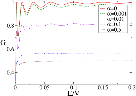
Figure 1: Dephasing in quantum double barrier system in 1D obtained from stochastic absorption model. The data is for two rectangular potential barrier having same width ($w_{1}=w_{2}=0.01$) and strength ($V_{1}=V_{2}=V=20)$. The intermediate distance between two barriers is $s=10$. We plot conductance $G$ (in units of $2e^{2}/h$) as a function of energy $E/V$. The SA gives $G=T/2$ in the incoherent limit of large $\alpha s$, $T$ being the transmittance through a single barrier.

II Double barrier

Let us assume a double barrier system consisting of two barriers characterized by transmittances $T_{1}$ and $T_{2}$. We consider the expression for two terminal conductance given by $G=T$ or equivalently the two terminal resistance ${\cal R}=1/T$. In the incoherent limit resistances should add as in Ohm’s law to give the total resistance: ${\cal R}=1/G=\sum_{i}1/T_{i}$ for a system of $i=1\dots n$ barriers connected in series.

To test the SA and RP models of dephasing let us take a one dimensional double barrier system consisting of two identical rectangular potential barriers of strength $V$ and width $w$. Let the two barriers be separated by a distance $s$. $k=\sqrt{2mE/\hbar^{2}}$ is the wave-vector and the imaginary wave-number is $\kappa=\sqrt{2m(V-E)/\hbar^{2}}$. The $S$-matrix elements for each of the rectangular barriers are,

$$t = \frac{-4ik}{2\kappa\sinh(\kappa w)(1-\frac{k^{2}}{\kappa^{2}})-4ik\cosh(\kappa w)},$$

$$r = \frac{\kappa+ik}{\kappa-ik}\left(-1+t\exp(-\kappa w)\right)$$ (2)

and the $S$-matrix is unitary and symmetric. In the SA model we assume that the propagator undergoes an attenuation $\exp(-\alpha s)$ in a single trip between the barriers. Thus the various elements of the combined S-matrix required to calculate the conductance in SA method are,

$$t_{12}=t^{2}\exp(-\alpha s+iks)/D,$$

$$r_{11}=r+t^{2}~{}r\exp(-2\alpha s+2iks)/D$$ (3)

with $t_{21}=t_{12}$, $r_{22}=r_{11}$. In the above expressions, $D=1-r^{2}\exp(-2\alpha s+2iks)$. Using these and Eq.(1) we find a loss of oscillation (coherence) in the total conductance along with a decay in total conductance as a function of $\alpha$ (See Fig.1). At large enough absorption $\alpha s\to\infty$ (practically already for $\alpha s\geq 5$) the total conductance asymptotically approaches the value $G\to T/2$, a result expected from the earlier discussions on incoherent limit ($1/G=1/T+1/T$).

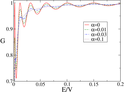
Figure 2: Dephasing in quantum double barrier system in 1D using random phase model. The system parameters are the same as in Fig.1. We plot conductance $G$ (in units of $2e^{2}/h$) as a function of energy $E/V$. The MC simulation predicts $G=T/(2-T)$ in the incoherent limit of large $\alpha s$, $T$ being the transmittance through a single barrier.

For the implementation of MC averaging over random phases, note that the transmittance through a single such barrier is $T=1/[1+(k^{2}+\kappa^{2})^{2}~{}\sinh^{2}(2\kappa w)/4k^{2}\kappa^{2}]$ and reflectance is $R=1-T$. We assume that the propagator picks up a random phase $\phi$ while traversing the free space ($s$) between the barriers, the total transmittance through the double barrier system. For each realization of the random phase, total transmittance across the double barrier system is

$$T_{12}=\frac{T^{2}}{1-2R\cos(2ks+2\phi)+R^{2}}.$$ (4)

The random phase is assumed to follow a Gaussian distribution of mean $\langle\phi\rangle=0$ and variance $\langle\phi^{2}\rangle=2\alpha s$. An average over $500$ realizations of the random phase is performed at each $\alpha$ to observe a monotonic decay of the oscillations (dephasing) in total conductance $G=\langle T_{12}\rangle$. In the limit of large dephasing factor $\alpha s\to\infty$ (practically already for $\alpha s\geq 1$) $G\to T/(2-T)$ (Fig.2). This is what one obtains by adding the $S$-matrices of the two barriers incoherentlydatta ; zheng . For two dissimilar barriers the RP method in the incoherent limit predicts $G=T_{1}T_{2}/(1-R_{1}R_{2})$, $G=T/(2-T)$ being a special case with $T_{1}=T_{2}=T$. This result is in clear disagreement with the expectation of Ohm’s law in series resistors in the limit of complete dephasing.

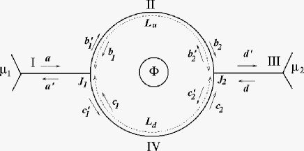
Figure 3: A schematic diagram of the 1D quantum ring considered. $\Phi$ denotes the flux enclosed. The arrows show counter propagating amplitudes of wave functions. $\mu_{1,2}$ chemical potentials at two reservoirs connecting the ring at the junctions $J_{1,2}$ by two leads.

III Quantum ring

We consider a quantum ring (Fig.3) where $L_{u},~{}L_{d}$ are the lengths of the upper and lower arms respectively. The total circumference of the ring is $L=L_{u}+L_{d}$. The ring is connected to two leads at junctions $J_{1}$ and $J_{2}$. These connections are described by a scattering matrix $S_{c}$. For the junction $J_{1}$ the outgoing amplitudes $(a^{\prime},b^{\prime}_{1},c^{\prime}_{1})$ are connected to the incoming amplitudes $(a,b_{1},c_{1})$ via $S_{c}$. Similarly for junction $J_{2}$, $(d^{\prime}~{}b^{\prime}_{2}~{}c^{\prime}_{2})^{T}=S_{c}(d~{}b_{2}~{}c_{2})^{T}$. The junction S-matrices can be modeled asazbel

$$S_{c}=\left(\begin{array}[]{ccc}-(p+q)&\sqrt{\epsilon}&\sqrt{\epsilon}\\ \sqrt{\epsilon}&p&q\\ \sqrt{\epsilon}&q&p\end{array}\right)$$ (8)

with $p=[\sqrt{1-2\epsilon}-1]/2$ and $q=[\sqrt{1-2\epsilon}+1]/2$. The $S$-matrix $S_{c}$ is characterized by a single parameter $\epsilon$, which can take any value from $0$ (decoupled) to $0.5$ (strongly coupled). The quantum mechanical continuity of wave-function and its derivative is attained at the junctions for $\epsilon=4/9$. Without any lack of generality we use this value for the coupler $\epsilon$ in our study.

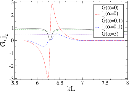
Figure 4: Results from stochastic absorption in quantum ring with $L_{u}/L=0.45$ and $L_{d}/L=0.55$ in absence of magnetic flux. The coupler $\epsilon=4/9$. Conductance $G$ (in units of $2e^{2}/h$) and circulating current density $j_{c}$ (in units of $j_{in}$, see text) in a open quantum ring with changing Fermi momentum $kL$. The amount of circulating current $j_{c}$ and the range of energy over which it is obtained reduces with increase in dephasing $\alpha$. At large enough $\alpha(=5)$ $G\to\epsilon$.

The amplitudes $b_{1},b_{2}$ and $b_{1}^{\prime},b_{2}^{\prime}$ of the upper arm are related by an $S$-matrix

$$\left(\begin{array}[]{c}b_{1}\\ b_{2}\end{array}\right)=\left(\begin{array}[]{cc}0&e^{i(k-\theta/L)\,L_{u}}\,P_{u}\\ e^{i(k+\theta/L)\,L_{u}}\,P_{u}&0\end{array}\right)\left(\begin{array}[]{c}b_{1}^{\prime}\\ b_{2}^{\prime}\end{array}\right).$$ (15)

Similarly for lower arm

$$\left(\begin{array}[]{c}c_{1}\\ c_{2}\end{array}\right)=\left(\begin{array}[]{cc}0&e^{i(k+\theta/L)\,L_{d}}\,P_{d}\\ e^{i(k-\theta/L)\,L_{d}}\,P_{d}&0\end{array}\right)\left(\begin{array}[]{c}c_{1}^{\prime}\\ c_{2}^{\prime}\end{array}\right).$$ (22)

Here $k\,L_{u}$ ($k\,L_{d}$) denotes the phase picked up by the electron while traversing the upper (lower) arm of the ring in absence of magnetic flux and any dephasing factor. In presence of Aharonov-Bohm flux ($\Phi$) phase of the wave-function in upper (lower) arm gets shifted by an amount $\theta\,L_{u}/L$ ($\theta\,L_{d}/L$). This phase-shift in two arms add up to give the total flux piercing the ring i.e. $\theta\,L_{u}/L+\theta\,L_{d}/L=2\,\pi\,\Phi/\Phi_{0}$, where $\Phi_{0}=h\,c/e$, flux quanta. An extra factor $P_{u}$ ($P_{d}$) in the propagator along the upper (lower) arm introduces dephasing in the system.

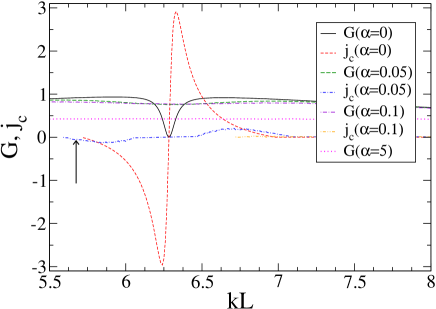
Figure 5: Results from random phase model in the quantum ring. Conductance $G$ (in units of $2e^{2}/h$) and circulating current density $j_{c}$ (in units of $j_{in}$) in a open quantum ring as a function of Fermi momentum $kL$. With increase in $\alpha$ amount of $j_{c}$ decreases. Notice the occurrence of $j_{c}\neq 0$ for $\alpha=0.05$ at some Fermi momenta (e.g. as denoted by the arrow) although for $\alpha=0$ at the same momenta $j_{c}=0$. At the incoherent limit of large $\alpha(=5)$ conductance obtained from MC averaging is $G<\epsilon$. The parameters used are $L_{u}/L=0.45,~{}L_{d}/L=0.55$ and $\epsilon=4/9$.

Before going into the calculation of conductance and impact of dephasing due to the two dephasing-models we study, let us first discuss what we expect in the completely incoherent limit. The incoming beam transits electrons in the upper (lower) arm with transmission coefficient $\epsilon$. Hence the upper (lower) arm have same resistances at the two junctions $1/\epsilon$. In the incoherent limit the resistances in upper (lower) arm add as in Ohm’s law, ${\cal R}_{u}=2/\epsilon$. Now these resistances add in parallel leading to the total conductance $G=2/{\cal R}_{u}=\epsilon$.

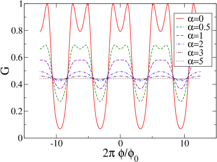
Figure 6: Stochastic absorption results in Aharonov-Bohm oscillations. The ring geometry is $L_{u}/L=0.45$, $L_{d}/L=0.55$. The coupler strength $\epsilon=4/9$. We fixed $kL=5$. The visibility of AB oscillations in $G$ (in units of $2e^{2}/h$) clearly dies out with increasing $\alpha$ to asymptotically reach a flux independent conductance $G=\epsilon$ in the limit of large $\alpha(=5)$.

In the method of stochastic absorption $P_{u}=\exp(-\alpha L_{u})$ and $P_{d}=\exp(-\alpha L_{d})$ act as the continuous lossy channels leading to dephasing. Thus combining these $S$-matrices one can obtain the elements of the effective two terminal ‘non-unitary’ $S$-matrix and using Eq.(1) find out the conductance $G$ in presence of lossy channels. In absence of magnetic flux ($\theta=0$) we study the conductance across an asymmetric ring ($L_{u}\neq L_{d}$). Throughout this analysis we use $L_{u}=0.45$ and $L_{d}=0.55$ in units of $L=L_{u}+L_{d}=1$. The conductance in such an asymmetric ring is known to show Fano-resonances as well as Breit-Wigner line shapes as a function of Fermi energycm-deo ; cm-pareek ; cm-sw . The Fano resonances accompany occurrences of circulating current in the ring. In presence of transport current through an asymmetric ring system, depending on Fermi-energy, in one of the arms current can be larger than the transport current. Thus it is known as current magnificationcm-deo ; cm-pareek ; cm-sw . In such a case, to maintain current conservation, in the other arm, current flows opposite to the bias. The amount of current flowing opposite to the bias (negative current) in upper and lower arms of the ring gives the magnitude of circulating current density $j_{c}$. We assign positive (negative) sign to $j_{c}$ for clockwise (anti-clockwise) circulating current density i.e. negative current density in lower (upper) arm $j_{d}<0$ ($j_{u}<0$). We measure the current densities in the unit of incident current density $j_{in}$. In a small energy interval $dE$ about the Fermi energy, the incident current density is $j_{in}=ev\frac{dn}{dE}f(E)dE$, where $f(E)$ is the Fermi distribution function, $\frac{dn}{dE}=2/hv$ is the density of states (DOS) in the perfect wire and $v=\hbar k/m$. For the zero temperature calculations $f(E)=1$ for occupied states. Thus the incident current density becomes $j_{in}=(2e/h)dE$. In dimensionless units the current density in upper (lower) arm is $j_{u}/j_{in}=|b^{\prime}_{1}|^{2}-|b_{1}|^{2}=|b_{2}|^{2}-|b^{\prime}_{2}|^{2}$ ($j_{d}/j_{in}=|c^{\prime}_{1}|^{2}-|c_{1}|^{2}=|c_{2}|^{2}-|c^{\prime}_{2}|^{2}$).

Occurrence of circulating current is a purely quantum phase coherence effect. Thus with increasing dephasing the circulating current density is expected to decay, vanishing completely for fully incoherent transport. So we focus on the change in this quantity with increasing $\alpha$ to quantify the degree of dephasing introduced by the two dephasing models at hand. Fig.4 shows the total conductance $G$ and the circulating current density $j_{c}$ as a function of Fermi momentum ($kL$) in absence ($\alpha=0$) and presence ($\alpha=0.1$) of dephasing. It is clear from the figure that amount of the circulating current density $j_{c}$ and the range of Fermi momentum over which it is found, decreases with increasing $\alpha$. It is assumed here that the reinjected current which leads to classical behaviour does not contribute to circulating current. At the $\alpha\to\infty$ limit it is found that $G\to\epsilon$ [see $G^{sa}(\alpha=5)$ in Fig.4]. In this limit the circulating current density is completely absent. Thus predictions from SA is completely consistent with our expectations about the incoherent limit.

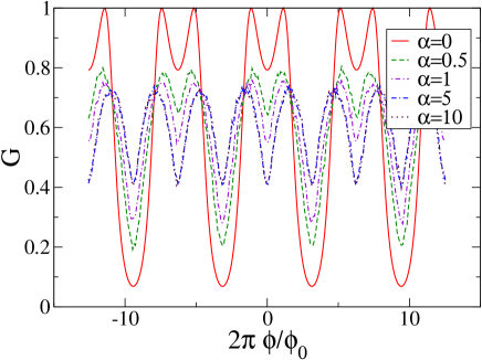
Figure 7: Results of random phase model in Aharonov-Bohm oscillations. The parameters used are $L_{u}/L=0.45,~{}L_{d}/L=0.55,~{}kL=5$ and $\epsilon=4/9$. The method clearly fails to reduce the visibility of AB oscillations in $G$ (in units of $2e^{2}/h$) with increasing $\alpha$ beyond $5$.

In the RP model, on the other hand, a random phase is picked up by the propagator while traversing the two arms of the ring. Dephasing in this model is introduced by $P_{u}=\exp(i\phi_{u})$ and $P_{d}=\exp(i\phi_{d})$ such that the phases obey Gaussian distributions with zero mean and variance $\sigma_{u}^{2}=2\alpha L_{u}$ and $\sigma_{u}^{2}=2\alpha L_{d}$. At each realization of the random phases the $S$-matrices connecting the left and right junctions (Eqs. (15) and (22)) are unitary and symmetric. Thus they obey Onsager reciprocitydatta at each given realization. In this method one needs to find the transmittance $T_{12}$ in each realization and perform an MC averaging over various realizations. We averaged over $500$ realizations for each value of $\alpha$. From Fig.5 it is clear that this method is also capable of reducing the amount of circulating current density for most of the Fermi momenta. However, at some regimes of Fermi momenta, e.g. near $kL=5.6$, we now observe non-zero $j_{c}$ in presence of non-zero $\alpha$(=0.05) though at the same points with $\alpha=0$ circulating current density was absent (Fig.5). This clearly goes against the basic notion of dephasing – as this is enhancement of an effect (circulating current) purely attributed to phase coherencecm-sw . SA method is seen to be free from such discrepancies. However at large enough $\alpha$(=5) the circulating current density completely vanishes and the total conductance becomes independent of $kL$. The $\alpha\to\infty$ limit of $G$ obtained by this method remains slightly smaller than that obtained in SA method ($G<\epsilon$, see Fig.5).

Next we switch on the magnetic flux $\Phi$ and study how dephasing affects the Aharonov-Bohm (AB) oscillations of conductance $G$ as a function of magnetic flux. The SA absorption method leads to a monotonic decay in the visibility of oscillations (difference between maxima and minima) with increasing $\alpha$ (Fig.6) eventually the conductance becoming independent of $\Phi$ in the limit $\alpha L\to\infty$. In fact at $\alpha L=5$ it reaches the incoherent limit of $G\to\epsilon$. On the other hand, though the RP model leads to dephasing at small $\alpha$, it rapidly saturates and fails to kill the AB oscillation with increasing $\alpha$ any further.

\psfrag{ai}{\Large{$a_{i}$}}\psfrag{a1}{\large{$a_{1}$}}\psfrag{a2}{\large{$a_{2}$}}\psfrag{a3}{\large{$a_{3}$}}\psfrag{al}{\Large{$\alpha$}}\includegraphics[width=227.62204pt]{sa-harms.eps}

Figure 8: First three harmonics $a_{i}$, $i=1,2,3$ of $G$ as a function of dephasing factor $\alpha$. Result from stochastic absorption.

To understand the results, we explicitly extract the various harmonics in the conductance data presented above. The $n$-th harmonic is

$$a_{n}=\frac{1}{\pi}\int_{0}^{2\pi}G\cos(n\theta)d\theta.$$ (23)

The SA method shows fast decay in the various harmonics. In Fig.8 it is clearly seen that the higher is the harmonic the faster it decays to zero with increasing $\alpha$. However, the same first three harmonics from MC data shows a different behavior (Fig.9). All the odd harmonics decay to zero, higher harmonics going to zero faster than the lower one. Whereas the even harmonics show an initial decay followed by a saturation. It is clear from Fig.9 that the second harmonic $a_{2}$ saturates to $a_{2}=-0.14$ with increasing $\alpha$. Therefore the AB oscillation that was predominantly $\Phi_{0}$ oscillation at $\alpha L=0$ becomes predominantly a $\Phi_{0}/2$ oscillation for $\alpha L>5$ (Fig.7). In fact, the RP model fails to kill all the even harmonics in the AB oscillations.

This failure of RP model can be understood in the following way. Consider two paths which are time reversed version of each other. Start from a point to go around the ring (clockwise) once and come back to origin. One can also travel anticlockwise and come back to the same point. These are the two time reversed paths. These two paths together encloses the flux twice. This leads to the $\Phi_{0}/2$ oscillation as a function of magnetic flux. Notice that the phase difference, due to the magnetic flux, between these two paths is $4\pi\Phi/\Phi_{0}$. However, due to the symmetric nature of the phase randomizing $S$-matrix, each of these two paths picks up the same random phase. Thus in the phase difference, the contribution from random phase cancels out. Therefore phase randomization in the RP model fails to kill even periodicity ($\Phi_{0}/2n$ with integer n) contributions in one dimensional geometries. This is true for all even harmonics.

\psfrag{ai}{\Large{$a_{i}$}}\psfrag{a1}{\large{$a_{1}$}}\psfrag{a2}{\large{$a_{2}$}}\psfrag{a3}{\large{$a_{3}$}}\psfrag{al}{\Large{$\alpha$}}\includegraphics[width=227.62204pt]{mc-harms.eps}

Figure 9: First three harmonics $a_{i}$, $i=1,2,3$ of $G$ as a function of dephasing factor $\alpha$. Result from random phase model.

IV Discussions and conclusion

Studies on series and parallel geometry showed that the SA method leads to monotonic dephasing (decay in visibility of oscillations or purely coherent effect like circulating current densities in the ring) with increase in dephasing parameter $\alpha$. In the fully incoherent limit of $\alpha\to\infty$ we recover Ohm’s law, inverse transmittance through individual elements (a barrier in double barrier case and an arm in quantum ring) behaving as classical resistances. On the other hand RP model of introducing random phases to the propagator and averaging over many realizations leads to several inconsistencies. For double barrier transmittance, this leads to an incoherent limit that differs from the classical Ohm’s law. For the transmission through quantum ring, this method generates circulating current in some regimes of Fermi wave-vectors where there was no circulating current in absence of phase randomization. This behavior is clearly beyond the very principle of dephasing, as the circulating current is of purely quantum mechanical origin. If the ring is penetrated by magnetic flux, RP model fails to kill the $\Phi_{0}/2$ oscillations. This is because RP model fails to dephase interference between complementary electron waves which follow time reversed path of each other.

Thus in conclusion, we find the SA method to be a reliable phenomenological technique of introducing dephasing. This systematically increases dephasing with increasing value of the dephasing parameter $\alpha$, finally leading to classical Ohm’s law in the limit of large $\alpha$. However the RP model fails in many aspects to be a useful phenomenological model of dephasing.

V Acknowledgment

We thank Martina Hentschel for useful comments on the manuscript.

References

- (1) Y. Imry, Introduction to mesoscopic physics, 2nd ed. (Oxford University press, Oxford, 2002).
- (2) M. Büttiker, Phys. Rev. B 33, 3020 (1986).
- (3) M. Büttiker, IBM J. Res. Dev. 32, 63 (1988).
- (4) D. Roy and A. Dhar, Phys. Rev. B 75, 195110 (2007).
- (5) Y. Zohta and H. Ezawa, J. Appl. Phys. 72, 3584 (1992).
- (6) A. Rubio and N. Kumar, Phys. Rev. B 47, 2420 (1993).
- (7) A. M. Jayannavar, Phys. Rev. B 49, 14 718 (1994).
- (8) A. K. Gupta and A. M. Jayannavar, Phys. Rev. B 52, 4156 (1995).
- (9) S. K. Joshi, D. Sahoo, and A. M. Jayannavar, Phys. Rev. B 62, 880 (2000).
- (10) P. W. Brouwer and C. W. J. Beenakker, Phys. Rev. B 55, 4695 (1997).
- (11) S. Datta, Electronic transport in mesoscopic systems (Cambridge University press, Cambridge, 1997).
- (12) C. Benjamin and A. M. Jayannavar, Phys. Rev. B 65, 153309 (2002).
- (13) C. Benjamin, S. Bandopadhyay and A. M. Jayannavar, Solid State Commun. 124, 331 (2002).
- (14) A. Fuhrer et al., Phys. Rev. B 73, 205326 (2006).
- (15) M. G. Pala and G. Iannaccone, Phys. Rev. B 69, 235304 (2004).
- (16) H. Zheng, Z. Wang, Q. Shi, X. Wang, and J. Chen, Phys. Rev. B 74, 155323 (2006).
- (17) D. Roy and N. Kumar, Phys. Rev. B 76, 092202 (2007).
- (18) A. M. Jayannavar and P. SinghaDeo, Phys. Rev. B 51, 10175 (1995).
- (19) S. Bandopadhyay, P. S. Deo, and A. M. Jayannavar, Phys. Rev. B 70, 075315 (2004).
- (20) M. Büttiker, Y. Imry, and M. Y. Azbel, Phys. Rev. A 30, 1982 (1984).
- (21) T. P. Pareek, P. S. Deo, and A. M. Jayannavar, Phys. Rev. B 52, 14657 (1995).