Phase diagram of the one dimensional anisotropic Kondo-necklace model

Abstract

The one dimensional anisotropic Kondo-necklace model has been studied by several methods. It is shown that a mean field approach fails to gain the correct phase diagram for the Ising type anisotropy. We then applied the spin wave theory which is justified for the anisotropic case. We have derived the phase diagram between the antiferromagnetic long range order and the Kondo singlet phases. We have found that the exchange interaction ($J$) between the itinerant spins and local ones enhances the quantum fluctuations around the classical long range antiferromagnetic order and finally destroy the ordered phase at the critical value, $J_{c}$. Moreover, our results show that the onset of anisotropy in the XY term of the itinerant interactions develops the antiferromagnetic order for $J<J_{c}$. This is in agreement with the qualitative feature which we expect from the symmetry of the anisotropic XY interaction. We have justified our results by the numerical Lanczos method where the structure factor at the antiferromagnetic wave vector diverges as the size of system goes to infinity.

I Introduction

Quantum phase transitions between Kondo singlet and antiferromagnetically ordered states such as found in heavy fermion compounds have been attracted much research interest recently Continentino05 ; Vojta03 ; Fulde06 . It is therefore of great importance to understand the approach to the quantum critical region within suitable theoretical models. The most important among them is the Kondo lattice model consisting of a free conduction band and an on-site antiferromagnetic Kondo interaction which favors non-magnetic singlet formation. In the second order it also leads to the effective inter-site Ruderman-Kittel-Kasuya-Yosida (RKKY) interactions which favor magnetic order. Their competition leads to the appearance of the quantum critical point. In such a picture only spin degrees of freedom are involved in the quantum phase transition. Therefore the Kondo lattice model may be replaced by a simpler model where the itinerant hopping part is simulated by an inter-site interaction of the itinerant spins. Kondo necklace (KN) model has been originally proposed by Doniach Doniach77 for the one-dimensional case as a simplified version of the itinerant Kondo lattice (KL) model Tsunetsugu97 . Thereby the kinetic energy of conduction electrons is replaced by an intersite exchange term. For a pure XY-type intersite exchange this may be obtained by a Jordan-Wigner transformation. The intuitive argument is that at low temperatures the charge fluctuations in the Kondo lattice model are frozen out and the remaining spin fluctuation spectrum can be simulated by an antiferromagnetic inter-site interaction term of immobile $\tau$ spins coupled by a Kondo interaction to the local noninteracting spins $S$.

The quantum phase transition between the spin liquid and antiferromagnetic phases in the one dimensional Kondo necklace model has been studied by several methods jullien ; scalettar ; moukouri . The phase diagram of the genuine Kondo necklace model has been studied by mean field approach Zhang00 in spatial dimension D=1, 2, 3. The one dimensional case is always in the Kondo singlet phase which is justified by the numerical Monte-Carlo scalettar and Density Matrix Renormalization Group moukouri (DMRG) results. While a quantum phase transition between the Kondo singlet phase and the antiferromagnetic (AF) ordered phase happens by increasing the ratio ($t/J$) of inter-site to the local exchange interaction for D=2, 3. The effect of both intersite and intrasite anisotropies on the quantum critical point have also been investigated by the same approach langari-thalmeier . Mean field theory has also been applied to study the effect of magnetic field on the Kondo necklace model thalmeier-langari . However, for D=1 the mean field approach always shows a non-magnetic Kondo singlet phase even in the presence of anisotropy in the easy axis term langari-thalmeier .

In the present work we want to study the possible quantum phase transition in the D = 1 Kondo-necklace model under the assumption of the anisotropy in the XY-interaction ($\eta$) between the spin of itinerant electrons. However, the real space renormalization group (RG) study saguia shows that if the anisotropy in the XY-interaction is greater than some nonzero value a phase transition from the Kondo singlet to the antiferromagnetic long range order takes place by changing the local exchange coupling ($J/t$). It means that for $\eta<\eta_{c}$ the system is always in Kondo singlet state but for $\eta>\eta_{c}$ there is a critical exchange coupling ($J_{c}/t$) which is the border between the Kondo singlet and AF long range ordered phases. However, we will show that the quantum phase transition between the Kondo singlet and AF order exists for any nonzero value of $\eta$. Our result is based on the spin wave approach which is justified in the absence of local exchange for the anisotropic case. This is in agreement with the general statement which tells us about the universality of this transition. Moreover, the Lanczos numerical computations justify that our statement is correct.

In Sec.II we will explain why the mean field approach fails to produce the correct results in one spatial dimension and easy axis anisotropy. We then consider a more general case of anisotropy in the Hamiltonian in Sec.III. We then implement a spin wave theory to the Hamiltonian with anisotropy in Sec.IV and show that the local exchange will increase the quantum fluctuations which destroy the AF ordered state. In Sec.V we present our numerical Lanczos results which verifies our proposed phase diagram. Finally, the conclusion and discussion are presented in Sec.VI.

II Mean field theory

In this section we shortly review the mean field approach to the Kondo-necklace model. We will show that this approach fails to represent the antiferromagnetic phase for Ising like anisotropy. Let first consider the following Hamiltonian

$$\mathcal{H}_{\rm AKN}=t\sum_{\langle ij\rangle}\left(\tau_{i}^{x}\tau_{j}^{x}+\tau_{i}^{y}\tau_{j}^{y}+\delta\tau_{i}^{z}\tau_{j}^{z}\right)+J\sum_{i}\tau_{i}\cdot S_{i},$$ (1)

where $t$ is the strength of exchange coupling between the spin ($\tau$) of itinerant electrons and $J$ is exchange coupling between the spin of itinerant electrons and localized spins ($S$). The anisotropy parameter is represented by $\delta$. The bond operator representation Sachdev90 is used to transform the spin operators in terms of bosonic operators langari-thalmeier ($s,t_{x},t_{y},t_{z}$). We start from the strong coupling limit where the mean field theory works well and the model has a Kondo singlet ground state. For the mean field approach langari-thalmeier we assume a singlet condensation $\langle s\rangle=\bar{s}$ and a condensation for one triplet component to induce the antiferromagnetic order $t_{k,z}=\sqrt{N}\bar{t}\delta_{k,Q}+\eta_{k,z}$, where $\eta_{k,z}$ is the quantum fluctuation above the triplet condensation and $Q=\pi$. After performing the Bogoliubov transformation the Hamiltonian in momentum space becomes

$$\mathcal{H}^{mf}_{AKN}=E_{0}^{AF}+\sum_{k}[\sum_{\alpha=x,y}\omega_{\alpha}(k){\tilde{t}}^{\dagger}_{k,\alpha}{\tilde{t}}_{k,\alpha}+\omega_{z}(k){\tilde{\eta}}^{\dagger}_{k,z}{\tilde{\eta}}_{k,z}]$$ (2)

where $E_{0}^{AF}$ is the ground state energy, $\omega_{\alpha}(k)$ are the excitation energies ($\alpha=x,y,z$) and ${\tilde{t}}^{\dagger}_{k,x(y)}$, ${\tilde{\eta}}^{\dagger}_{k,z}$ (${\tilde{t}}_{k,x(y)}$, ${\tilde{\eta}}^{\dagger}_{k,z}$ ) are the bosonic creation (annihilation) operators in the diagonal representation. (More details can be found in Ref.langari-thalmeier, ). The excitation energies are

$$\omega_{\alpha}(k)=\sqrt{d_{\alpha}^{2}(k)-4f_{\alpha}^{2}(k)},\hskip 14.22636pt\alpha=x,y,z.$$ (3)

where

$$f_{x}(k) = f_{y}(k)=\frac{t\bar{s}^{2}}{4}\gamma(k),$$

$$d_{x}(k) = d_{y}(k)=\mu+\frac{J}{4}+\frac{t\bar{s}^{2}}{2}\gamma(k),$$

$$f_{z}(k) = \frac{t\bar{s}^{2}}{4}\delta\gamma(k),\hskip 2.84526ptd_{z}(k)=\mu+\frac{J}{4}+\frac{t\bar{s}^{2}}{2}\delta\gamma(k),$$ (4)

and $\gamma(k)=\cos(k)$. The ground state energy is

$$E_{0}^{AF}=E_{0}+N\bar{t}^{2}\left[\mu+\frac{J}{4}-t\bar{s}^{2}\delta\right],$$ (5)

where

$$E_{0}=N\Big{(}(\mu-\frac{3J}{4})\bar{s}^{2}-\mu\Big{)}+\frac{1}{2}\sum_{k,\alpha=x,y,z}\Big{(}\omega_{\alpha}(k)-d_{\alpha}(k)\Big{)}.$$ (6)

The chemical potential ($\mu$) has been added as a Lagrange multiplier to the mean field Hamiltonian to preserve the dimension of Hilbert space on each bond. The ground state energy should be minimized with respect to $\bar{s}$, $\bar{t}$ and $\mu$. It gives the following equations

$$\mu=t\delta\bar{s}^{2}-\frac{J}{4},$$

$$\bar{t}^{2}=\frac{5}{4}-\frac{J}{2t\delta}-\frac{1}{4N}\sum_{k}\Big{(}\frac{1}{\sqrt{1+\gamma(k)}}+\frac{2}{\sqrt{1+\frac{\gamma(k)}{\delta}}}\Big{)},$$

$$\bar{s}^{2}=\frac{5}{4}+\frac{J}{2t\delta}-\frac{1}{4N}\sum_{k}\Big{(}\sqrt{1+\gamma(k)}+2\sqrt{1+\frac{\gamma(k)}{\delta}}\Big{)},$$

(7)

which should be solved self consistently. For $\delta>1$, we expect to have the long range antiferromagnetic order in $z$ direction. However, the summation $\frac{1}{N}\sum_{k}\frac{1}{\sqrt{1+\gamma(k)}}$ in Eq.(7) diverges which shows that the mean field approach fails to work correctly in this case.

We have even considered the extreme case of only an Ising term in the interaction between itinerant spins, namely $t\rightarrow 0$ and $t\delta=constant$. It is clear that for $J=0$ the ground state is long ranged antiferromagnetic ordered. However, the above mean field theory fails to show the nonzero AF ordering. We conclude that the mean field theory is not suitable to show the long ranged antiferromagnetic phase in one dimension. It should be related to the strong quantum fluctuations which have dominant effect in one dimension. Moreover, the above mean field theory starts from the strong coupling limit ($t=0$) where the singlet condensation is supposed to be the case while for the antiferromagnetic phase we need to consider the weak coupling limit ($J=0$). Having this in mind, we start from the weak coupling limit with an AF ordered ground state for the Ising anisotropy case. The effect of nonzero local exchange ($J\neq 0$) increases the quantum fluctuations which finally destroy the AF long range order. In this respect, we apply the spin wave theory to the anisotropic Kondo necklace chain.

III The model Hamiltonian

The Hamiltonian defined in Eq.(1) is always in the Kondo singlet phase for XY anisotropy ($\delta\leq 1$) while it is expected to have a quantum phase transition to the AF ordered state at a critical exchange coupling ($\frac{J}{t}|_{c}$) for Ising anisotropy ($\delta>1$). To consider a general case we will investigate the phase diagram of the following Hamiltonian in one dimension

$$\mathcal{H}=t\sum_{i=1}^{N}(\tau_{i}^{z}\tau_{i+1}^{z}+(1-\eta)\tau_{i}^{y}\tau_{i+1}^{y})+J\sum_{i=1}^{N}(\overrightarrow{\tau_{i}}\cdot\overrightarrow{S_{i}}),$$ (8)

where $\eta$ is the anisotropy parameter which defines the deviation from the Ising limit ($\eta=1$). The main reason to consider the anisotropy in this form is that the anisotropy in the itinerant part of the interaction enables us to investigate the effect of symmetry on the results of the Kondo necklace model compared with the Kondo model. The present model, the case of $\eta=0$ has U(1) symmetry and for $\eta\neq 0$ it has Z2 symmetry. In the case of full anisotropy ($\eta=1$, Ising limit) we expect to have a quantum phase transition from the antiferromagnetic long range order to the Kondo singlet phase. Moreover, in the absence of local exchange coupling ($J=0$) the universal behavior of the XY term is the same as for all $\eta\neq 0$. It is also another motivation to see what is the effect of $\eta$ anisotropy on the phase diagram of the model. Specially, our final results show that there exist an antiferromagnetic phase for any nonzero value of $\eta$ when $J$ is smaller than the critical exchange coupling $J_{c}(\eta)$. The latter result is in contradiction with the renormalization group result presented in Ref.saguia, .

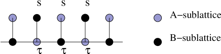
Figure 1: (Color online) One dimensional Kondo-necklace lattice labeled by two sublattices.

IV Spin wave approach

The spin wave theory is constructed on a ground state which is maximally polarized. The low-lying excitations are expected to be created by flipping a spin and letting this disturbance to propagate in the crystal which is a spin wave. These excitations are called magnons which are bosonic quasi particles.

To apply the spin wave approach the one dimensional Kondo-necklace lattice is labeled by two sublattices A and B (see Fig.1). The Hamiltonian (8) can be written in the following form where $\sum_{\sigma}$ represents the summation over the nearest neighbors

$$\mathcal{H}=t\sum_{i=1}^{N/2}\sum_{\sigma}(\tau_{i}^{zA}\tau_{i+\sigma}^{zB}+(1-\eta)\tau_{i}^{yA}\tau_{i+\sigma}^{yB})$$

$$+J\sum_{i=1}^{N/2}(\overrightarrow{\tau_{i}}^{A}\cdot\overrightarrow{S_{i}}^{B}+\overrightarrow{\tau_{i}}^{B}\cdot\overrightarrow{S_{i}}^{A}).$$ (9)

We then implement the Holstein-Primakov transformation hp to write the spin operators in terms of bosonic operators. Starting from the weak coupling regime ($J=0$) the polarized ground state is the Neel state which impose the following transformations for spins of the itinerant electrons

$$\tau_{i}^{zA}=\tau-a_{i}^{\dagger}a_{i}\hskip 14.22636pt,\hskip 14.22636pt\tau_{i}^{zB}=-\tau+a_{i}^{\dagger}a_{i},$$ (10)

$$\tau_{i}^{+A}=(\sqrt{2\tau})(1-\frac{a_{i}^{\dagger}a_{i}}{2\tau})^{1/2}a_{i},$$

$$\tau_{i}^{+B}=(\sqrt{2\tau})a_{i}^{\dagger}(1-\frac{a_{i}^{\dagger}a_{i}}{2\tau})^{1/2},$$

$$\tau_{i}^{-A}=(\sqrt{2\tau})a_{i}^{\dagger}(1-\frac{a_{i}^{\dagger}a_{i}}{2\tau})^{1/2},$$

$$\tau_{i}^{-B}=(\sqrt{2\tau})(1-\frac{a_{i}^{\dagger}a_{i}}{2\tau})^{1/2}a_{i}.$$

In the above equations $\tau$ is the magnitude of spin and the Boson creation ($a^{\dagger}$) and annihilation ($a$) operators obey the following commutation relations,

$$[a_{i}^{\dagger},a_{j}]=\delta_{i,j}\hskip 5.69054pt,\hskip 5.69054pt[a_{i}^{\dagger},a_{j}^{\dagger}]=0\hskip 5.69054pt,\hskip 5.69054pt[a_{i},a_{j}]=0.$$ (11)

A similar transformations is also defined for the localized spin ($S$) by replacing $\tau\longrightarrow S$ and $a\longrightarrow e$ in Eqs.(10) where $e^{\dagger}$ ($e$) represents the creation (annihilation) Boson operator for the localized spins. Generally, one should define two types of Boson operators (in each sublattice) for both itinerant and localized spins. However, due to the translational invariance symmetry of the model the Boson operators for itinerant spins in each sublattice define the same operator as defined in Eqs.(10). The same story exists also for the localized ones.

The linear spin wave theory is implemented here where the spin operators are described in linear form of the Boson operators and higher order terms have been neglected,

$$\tau_{j}^{yA}\simeq\frac{\sqrt{2\tau}}{2i}(a_{j}-a_{j}^{\dagger})\hskip 5.69054pt,\hskip 5.69054pt\tau_{j}^{yB}\simeq\frac{\sqrt{2\tau}}{2i}(a_{j}^{\dagger}-a_{j}).$$ (12)

Similar expressions to Eq.(12) are applied for the other component of spin operators where they are replaced by Boson ones within the linear spin wave approximation which finally leads to the following form for the whole Hamiltonian

$$\mathcal{H}=-N(t\tau^{2}+J\tau S)+t\tau\sum_{i=1}^{N/2}\sum_{\sigma}(2a_{i}^{\dagger}a_{i}+a_{i+\sigma}^{\dagger}a_{i+\sigma})$$ (13)

$$- \frac{t\tau(1-\eta)}{2}\sum_{i=1}^{N/2}\sum_{\sigma}(a_{i}a_{i+\sigma}^{\dagger}+a_{i}^{\dagger}a_{i+\sigma}-a_{i}^{\dagger}a_{i+\sigma}^{\dagger}-a_{i}a_{i+\sigma})$$

$$+ 2J\sum_{i=1}^{N/2}(Sa_{i}^{\dagger}a_{i}+\tau e_{i}^{\dagger}e_{i})+2J\sqrt{\tau S}\sum_{i=1}^{N/2}(a_{i}e_{i}+a^{\dagger}_{i}e^{\dagger}_{i}).$$

To proceed further and diagonalize the Hamiltonian we first transform the operators to their Fourier counterparts by the following relations,

$$a_{j}=\sqrt{\frac{2}{N}}\sum_{k}e^{ikj}c_{k}\hskip 14.22636pt,\hskip 14.22636ptc_{k}=\sqrt{\frac{2}{N}}\sum_{j}e^{-ikj}a_{j},$$ (14)

$$e_{j}=\sqrt{\frac{2}{N}}\sum_{k}e^{ikj}h_{k}\hskip 14.22636pt,\hskip 14.22636pth_{k}=\sqrt{\frac{2}{N}}\sum_{j}e^{-ikj}e_{j}.$$ (15)

In the momentum space representation and for $\tau=s=1/2$ the Hamiltonian (Eq.(13)) is finally written in the following form

$$\mathcal{H}=-\frac{N}{4}(1+J)+\frac{(1-\eta)}{4}\sum_{k}\gamma(k)[c_{k}^{\dagger}c_{-k}^{\dagger}+c_{k}c_{-k}]$$

$$+\frac{J}{2}\sum_{k}\Big{(}c_{k}h_{-k}+c_{-k}^{\dagger}h_{k}^{\dagger}+c_{-k}h_{k}$$

$$\hskip 99.58464pt+c_{k}^{\dagger}h_{-k}^{\dagger}+h_{k}^{\dagger}h_{k}+h_{-k}^{\dagger}h_{-k}\Big{)}$$

$$+\sum_{k}[(J/2+1)-\frac{(1-\eta)}{4}\gamma(k)][c_{k}^{\dagger}c_{k}+c_{-k}^{\dagger}c_{-k}].$$ (16)

The Hamiltonian can be diagonalized by the para-unitary transformation paraunitary for the general case of $\eta\neq 1$. However, for the case of $\eta=1$, one can use the Bogoliubov transformation which is a special case of the general para-unitary transformation.

IV.1 $\eta=1$

The Hamiltonian of the general case $\eta\neq 1$ can be diagonalized by the para-unitary transformation paraunitary for the bosonic operators. In this formalism the Hamiltonian is written as a hermitian 2m-square matrix $D$. The para-unitary transformation ($\Gamma$) can be constructed if and only if $D$ is positive definite. This procedure is presented in appendix.

However, for the special case $\eta=1$ the para-unitary transformation is the usual Boguliubov transformation bogolioubov . In this case, the bosonic operators is transformed to a new set of bosonic operators ($\alpha,\beta$) by the following relations,

$$c_{k}=u_{k}\alpha_{k}+v_{k}\beta^{\dagger}_{-k}\hskip 5.69054pt,\hskip 5.69054pth_{k}=u_{k}\beta_{k}+v_{k}\alpha^{\dagger}_{-k}$$ (17)

where $u_{k}=\cosh(\theta_{k})$ and $v_{k}=\sinh(\theta_{k})$ and $\theta_{k}$ is the free parameter of transformation. The parameter $\theta_{k}$ should satisfy the following relation to have a diagonal Hamiltonian

$$\mbox{tanh}(2\theta_{k})=\frac{-J}{J+1},$$ (18)

which is actually independent of $k$. The diagonalized Hamiltonian in terms of the new sets of operators is

$$\mathcal{H}=E_{0}(J)+\sum_{k}(\overline{\omega}_{\alpha}(k)\alpha_{k}^{\dagger}\alpha_{k}+\overline{\omega}_{\beta}(k)\beta_{k}^{\dagger}\beta_{k})$$ (19)

where the ground state energy is

$$E_{0}(J)=N[-\frac{5}{4}(1+J)+\sqrt{1+2J}],$$ (20)

and the quasiparticle excitations are

$$\overline{\omega}_{\alpha}(k)=-1+\sqrt{1+2J}\hskip 5.69054pt,\hskip 5.69054pt\overline{\omega}_{\beta}(k)=1+\sqrt{1+2J}.$$ (21)

The sublattice magnetization $m_{A}=\frac{2}{N}\sum_{i}\langle\tau-a_{i}^{\dagger}a_{i}\rangle$ defines the order parameter for the AF long range ordered phase which can be calculated in the diagonal bases of the Hamiltonian. For simplicity we put $t=1$ as the scale of energy. In the weak coupling limit $J=0$ the Hamiltonian (Eq.(8)) has long range AF order. The quantum fluctuations which are created by nonzero $J$ decrease the amount of AF ordering and finally destroy the ordered phase at a critical value, $J_{c}$, where the sublattice magnetization becomes zero

$$m_{A}=\frac{1}{2}-\langle a_{i}^{\dagger}a_{i}\rangle=1-\frac{J+1}{2\sqrt{1+2J}}=0\Longrightarrow J_{c}\simeq 6.46.$$ (22)

It is the first estimate of the critical value of the exchange coupling. However, the condition which we have stated is the extreme value where the quantum fluctuations suppress the sublattice magnetization totally. At this extreme condition the accuracy of the linear spin wave results is not justified, since the amplitude of the quantum fluctuations is not small. However, this approach is valid for small amplitude of fluctuations. Moreover, it shows that the amplitude of fluctuations become large by increasing the value of exchange coupling ($J$). Thus, the qualitative picture of the spin wave approximation is correct.

To justify that the spin wave theory gives correct results, we have plotted the ground state energy per site versus the exchange coupling ($J$) in Fig.2. We have compared the results obtained in Eq.(20) with the numerical Lanczos ones which will be discussed in the next section. It shows very good agreement of the spin wave with Lanczos results which justifies that the spin wave ground state presented here can be a good candidate to represent the many body ground state in this case.

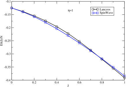
Figure 2: (Color online) Ground state energy per site ($E_{0}(J)/N$) versus $J$ for $\eta=1$ obtained by numerical Lanczos method (extrapolated to the $N\rightarrow\infty$ with 4 digits accuracy) and linear spin wave theory which show very good agreement.

IV.2 $\eta\neq 1$

We have implemented the para-unitary transformation (see appendix) to diagonalize the Hamiltonian (Eq.(IV)). The diagonalized Hamiltonian in terms of new sets of bosonic operators ($\phi,\psi$) is

$$\mathcal{H}=E_{0}(\eta,J)+\sum_{k}[\Omega_{\alpha}(k)\phi_{k}^{\dagger}\phi_{k}+\Omega_{\beta}(k)\psi_{k}^{\dagger}\psi_{k}].$$ (23)

where $E_{0}(\eta,J)=(1/N)\sum_{k}e_{0}(\eta,J;k)$ is the ground state energy and $e_{0}(\eta,J;k)$ has the following expression

$$e_{0}(\eta,J;k)=\frac{1}{2\sqrt{2}}\big{(}\sqrt{\mathcal{P}-\mathcal{Q}}+\sqrt{\mathcal{P}+\mathcal{Q}}\big{)},$$

$$\mathcal{P}=4(1+J)-(2+J)\gamma(k)\;\;,\;\;\mathcal{Q}=\sqrt{\mathcal{S}+\mathcal{T}^{2}},$$

$$\mathcal{S}=(2+J)\gamma(k)\eta-8J^{2}(2+\gamma(k)(\eta-1)),$$

$$\mathcal{T}=4+J(4+\gamma(k)(\eta-1))+2\gamma(k)(\eta-1).$$ (24)

The frequencies $\Omega_{\alpha}(k)$ and $\Omega_{\beta}(k)$ are

$$\Omega_{\alpha}(k)=\frac{1}{\sqrt{2}}\sqrt{4(1+J)-(2+J)\gamma(k)-\mathcal{A}}$$

$$\Omega_{\beta}(k)=\frac{1}{\sqrt{2}}\sqrt{4(1+J)-(2+J)\gamma(k)+\mathcal{A}},$$ (25)

where

$$\mathcal{A}=\sqrt{\mathcal{S}+\mathcal{T}^{2}}.$$ (26)

A remark is in order here, the results in this subsection will not reproduce the results of $\eta=1$ case simply by putting $\eta$ equal to one. The reason is related to a divergent factor of $(1-\eta)^{-1}$ which appears in the intermediate part of calculations. Such terms will not appear if we put $\eta=1$ from the beginning and the calculations will become much simpler as presented in the last subsection. In the diagonal bases of the Hamiltonian we can calculate the sublattice magnetization as defined in Eq.(10). As we have discussed in the previous subsection we can determine the critical border between the AF order and the Kondo singlet phase by looking for the position where the sublattice magnetization becomes zero.

Our results which are summerized in Table.1. show that the onset of nonzero XY-anisotropy ($\eta\neq 0$) develops the long range AF order for small local exchange coupling ($J<J_{c}$). This is also justified by the numerical Lanczos results where the static structure factor at momentum $\pi$ diverges for any nonzero $\eta$ and $J<J_{c}$. However, the numerical values for $J_{c}$ which are obtained by the spin wave approach is far from the numerical Lanczos ones. This will be discussed in the Sec.VI.

V Numerical Lanczos Results

The numerical Lanczos method has been applied to the one dimensional anisotropic Kondo-necklace model defined in Eq.(8). The anisotropic Hamiltonian does not commute with the total $z$-component spin. Thus, one should consider the full Hilbert space for doing numerics. In this respect, we have performed the numerical computations with $N=12,16,20,24$ spins. The computations have been done for different values of the exchange coupling ($J$) and the anisotropy parameter ($\eta$) to trace the quantum phase transition between the Kondo singlet phase and the antiferromagnetic one. The Kondo singlet ground state is not ordered while the antiferromagnetic phase has long range order. The long range order imposes that the structure factor diverges in the thermodynamic limit ($N\rightarrow\infty$) for the antiferromagnetic wave vector $k=\pi$. The structure factor of the $z$-component spin at the wave vector $k$ is defined by

$$G(k)=\sum_{r=0}^{\frac{N}{2}-1}\langle\tau_{0}^{z}\tau_{r}^{z}\rangle e^{ikr}.$$ (27)

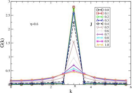
Figure 3: (Color online) The $z$-component structure factor versus $k$ for $\eta=0.6$, $N=24$ and different $J=0.0,0.1,0.2,\dots,1.0$.

We have plotted the structure factor ($G(k)$) versus the wave vector ($k$) for $\eta=0.6$, $N=24$ and different exchange couplings ($J=0.0,0.1,0.2,\dots,1.0$) in Fig.3. The structure factor gets a strong peak at $k=\pi$ for some values of $J$. This peak shows the presence of antiferromagnetic order. We will show in the next plots how the height of this peak evolve as the size of system changes.

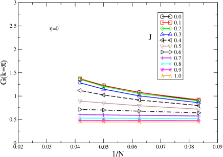
Figure 4: (Color online) The $z$-component structure factor for $k=\pi$ versus the inverse of of system size ($1/N$) for $\eta=0.0$ and different $J=0.0,0.1,0.2,\dots,1.0$. The structure factor diverges for $J=0$ like $\sqrt{N}$ which represent the massless behavior of XX spin 1/2 chain. The other sets of data show no divergence or weaker than $\sqrt{N}$ which justifies no long range antiferromagnetic order.

The $z$-component spin of structure factor at the antiferromagnetic wave vector, $k=\pi$, has been plotted in Figs.4-8 for different anisotropy ($\eta$) versus the inverse of system size ($N$). The system sizes are $N=12,16,20,24$. Each figure contains different plots for $J=0.0,0.1,0.2,\dots,1.0$.

We have plotted the case of genuine Kondo-necklace model, $\eta=0$ in Fig.4. For $J=0$, the properties of the XX spin 1/2 chain is reproduced which shows that the structure factor diverges karbach proportional to $\sqrt{N}$. However, it does not show the antiferromagnetic order of this model. It only represent the critical properties of the XX spin 1/2 chain which has algebraic decay of correlation functions. Turning on the local exchange to nonzero values $J\neq 0$ we observe weaker growth of the structure factor as the system size in increased. It is concluded that the one dimensional genuine Kondo-necklace model does not have an antiferromagnetic phase and is always in the Kondo singlet state. Moreover, we expect the structure factor diverges stronger than $\sqrt{N}$ for the antiferromagnetic ordered phase.

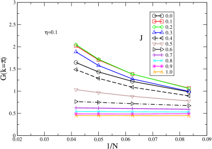
Figure 5: (Color online) The $z$-component structure factor versus $1/N$ (inverse of size of system) at $k=\pi$ for $\eta=0.1$ and different $J=0.0,0.1,0.2,\dots,1.0$. The divergence of $G(k=\pi)$ as $\frac{1}{N}\rightarrow 0$ for $J\leq 0.3$ is faster than $\sqrt{N}$. It shows the antiferromagnetic ordered phase for $J\leq 0.3$.

The presence of anisotropy ($\eta\neq 0$) breaks the U(1) symmetry and reduces it to Z2 symmetry. This is the onset of antiferromagnetic ordering formation which is the result of symmetry breaking. The structure factor at $k=\pi$ versus the inverse of length ($1/N$) for $\eta=0.1$ has been plotted in Fig.5. It is clear that $G(\pi)$ diverges faster than $\sqrt{N}$ for $J=0$ which verifies the formation of antiferromagnetic ordering in the ground state. A similar situation exists also for $J=0.1,0.2,0.3,0.4$. However, for $J\geq 0.5$ the divergence of $G(\pi)$ is not apparent as $N\rightarrow\infty$. We then conclude that for $J\leq J_{c}(\eta=0.1)\simeq 0.4$ the model has antiferromagnetic ordering while for larger values of $J$ it is in the Kondo singlet phase. Thus, a quantum phase transition occurs at $J_{c}$ from the antiferromagnetic order to the disordered Kondo singlet state.

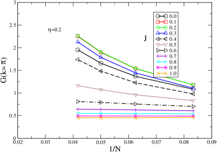
Figure 6: (Color online) $G(k=\pi)$ (the $z$-component structure factor) versus $1/N$ for $\eta=0.2$ and different $J=0.0,0.1,0.2,\dots,1.0$. It is clear that $G(k=\pi)$ diverges for $J<0.4$ as $N$ goes to infinity.

We have also plotted the z-component structure factor at antiferromagnetic wave length ($G(k=\pi)$) versus the inverse of system size ($1/N$) for $\eta=0.2$ in Fig.6, $\eta=0.6$ in Fig.7 and $\eta=1.0$ in Fig.8. We have observed that $G(k=\pi)$ diverges in the thermodynamic limit ($N\rightarrow\infty$) for $J\leq J_{c}(\eta)$ which verifies the existence of antiferromagnetic ordering. Our results for the critical exchange have been summerized in table.1. The accuracy of our results for the critical point ($J_{c}$) is about $\pm 0.05$. Because, the size of system is limited to $N=24$. To distinguish between the ordered and disordered phase more accurately it is necessary to consider larger system sizes.

Table 1: The critical exchange value ($J_{c}$) for different values of anisotropy ($\eta$). The Lanczos results are read from the data of $G(\pi)$ versus $1/N$ which has an accuracy about $\pm 0.05$.

$\eta$	0.1	0.2	0.6	1.0
$J_{c}$ (Lanczos)	0.3	0.35	0.4	0.45
$J_{c}$ (Spin Wave)	6.13	6.21	6.39	6.46

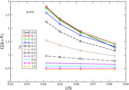
Figure 7: (Color online) The $z$-component structure factor versus $1/N$ for $k=\pi$ and $\eta=0.6$ and different $J=0.0,0.1,0.2,\dots,1.0$. The structure factor diverges for $J\leq 0.4$ and $\frac{1}{N}\rightarrow 0$.

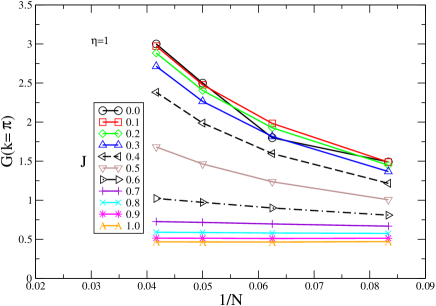
Figure 8: (Color online) The $z$-component structure factor versus $1/N$ at $k=\pi$ for $\eta=1.0$ and different $J=0.0,0.1,0.2,\dots,1.0$. The divergence of $G(k=\pi)$ for $N\rightarrow\infty$ is clear for $J<0.5$.

VI Conclusion and Discussion

We have studied the phase diagram of the one dimensional anisotropic Kondo necklace model. We have focused our attention on the case of Ising anisotropy (easy axis of the spin of itinerant electrons, $\delta>1$). Let us suppose that the interaction between the spin of itinerant electrons is only composed of $\tau^{z}_{i}\tau^{z}_{j}$ type. It is clear that in the absence of local exchange interaction ($J=0$) the model has a classical antiferromagnetic ordered ground state with nonzero staggered magnetization. It is expected that a nonzero local exchange ($J\neq 0$) adds quantum fluctuations which destroy the antiferromagnetic order at a critical exchange ($J_{c}$). However, the mean field approach langari-thalmeier fails to produce this picture correctly. In the mean field approach which is based on the strong coupling limit ($J/t\rightarrow\infty$) we have assumed a nonzero condensation for local singlet formation plus a nonzero triplet occupation ($\bar{t}$) which induces the antiferromagnetic order. The solution of the self consistent mean field equations always give no magnetic order, $\bar{t}=0$. A divergent integral appears if we assume $\bar{t}\neq 0$. However, the mean filed approach works fairly well in two and three dimensional models in addition to the case of XY anisotropy ($0<\delta<1$) of the one dimensional system langari-thalmeier .

To overcome the problem which appears in the mean field approach for Ising anisotropy of the one dimensional model we decided to start from the weak coupling limit ($J\rightarrow 0$). The linear spin wave theory has been implemented which is based on a classical antiferromagnetic ground state. To study the phase diagram we have considered a general case of Hamiltonian which has been given in Eq.(8). Our results show that the quantum fluctuations grow with increasing $J$ such that the sublattice magnetization becomes zero at a critical exchange coupling ($J_{c}$). Moreover, the antiferromagnetic phase exists for any nonzero value of anisotropy ($\eta\neq 0$) and $J<J_{c}$. It is in contradiction with the results presented in Ref.saguia, which gives the antiferromagnetic phase only for $\eta>\eta_{c}\simeq 0.58$. In other words our results state that $\eta_{c}=0$. We have plotted the phase diagram of the one dimensional anisotropic Kondo necklace model in the $J-\eta$ plane in Fig.9. It is obvious that for any nonzero $\eta$ there exists an antiferromagnetic phase. Moreover, the critical exchange coupling ($J_{c}$) depends strongly on $\eta$ for small anisotropy, $0<\eta<0.1$ while its dependence is weak for $\eta>0.1$.

Our result is in agreement with the symmetry arguments which is based on a qualitative picture. Let us first suppose that $J=0$. The remaining Hamiltonian is an anisotropic XY spin 1/2 chain. The quantum renormalization group langari verifies that the universality class of the nonzero anisotropy ($\eta\neq 0$) is the same as Ising case ($\eta=1$). Thus, if the antiferromagnetic phase exists for the Ising case it should also appear for any nonzero value of $0<\eta<1$. Moreover, the Hamiltonian has U(1) symmetry at $\eta=0$ while the symmetry is broken to the lower Z2 for $\eta\neq 0$. It is thus expected that the quantum phase transition happens at the symmetry breaking point. We expect that the addition of local exchange ($J\neq 0$) becomes irrelevant at the fixed point $J=0$, which is in agreement with our numerical results. However, this needs to be proved by more sophisticated methods like weak-coupling renormalization group which is out of the scope of this article.

Figure 9: Phase diagram of the one dimensional anisotropic Kondo necklace model where a quantum phase transition (dashed line) separates the ordered antiferromagnetic phase from the Kondo singlet one.

To verify that our result gives the correct phase diagram we have implemented the numerical Lanczos method. Our results show that the z-component structure factor diverges at the antiferromagnetic wave vector for any nonzero $\eta$ and $J<J_{c}$. However, the value of the quantum critical point ($J_{c}$) can not be determined with very high accuracy because of the finite size effect. In this study we have been limited to $N=24$ because the full Hilbert space should be considered in computation and the Lanczos is basically limited to such values. However, it is proposed that a density matrix renormalization group can get more accurate values. Moreover, we have understood that the critical exchange ($J_{c}$) which is given by spin wave theory is far from the real one which is given by numerical Lanczos method. The reason is related to the strong quantum fluctuations which exist close to critical point and ruin the accuracy of linear spin wave results.

VII Acknowledgments

This work was supported in part by the center of excellence in Complex Systems and Condensed Matter (www.cscm.ir). The authors acknowledge the support of Sharif University of Technology.

Appendix A The para-unitary transformation

This section is based on the approach proposed in Ref.paraunitary, to diagonalize a bosonic Hamiltonian. The Hamiltonian in Eq.(13) can be written in the following matrix form

$$\mathcal{H}=\sum_{k}\Gamma^{\dagger}D\Gamma$$ (28)

where $\Gamma^{\dagger}$ is a row vector

$$\Gamma^{\dagger}=(c^{\dagger}_{k}\hskip 5.69054pth^{\dagger}_{k}\hskip 5.69054ptc_{-k}\hskip 5.69054pth_{-k}),$$ (29)

and $D$ is a square matrix

$$D=\left(\begin{array}[]{cccc}\frac{2J+4-(1-\eta)\gamma(k)}{4}&0&\frac{(1-\eta)\gamma(k)}{4}&\frac{J}{2}\\ 0&\frac{J}{2}&\frac{J}{2}&0\\ \frac{(1-\eta)\gamma(k)}{4}&\frac{J}{2}&\frac{2J+4-(1-\eta)\gamma(k)}{4}&0\\ \frac{J}{2}&0&0&\frac{J}{2}\end{array}\right).$$ (34)

The Hamiltonian will be diagonalized by the following transformation ($\mathcal{J}$) to the new set of boson operators,

$$\Lambda=\mathcal{J}\Gamma,$$ (35)

where

$$\Lambda^{\dagger}=(\phi^{\dagger}_{k}\hskip 5.69054pt\psi^{\dagger}_{k}\hskip 5.69054pt\phi_{-k}\hskip 5.69054pt\psi_{-k}),$$ (36)

and the diagonal representation is given in Eq.(23). The new set of operators should satisfy the bosonic commutation relation, namely

$$[\Lambda_{i},\Lambda^{\dagger}_{j}]=\hat{\delta}_{i,j},$$ (37)

where $\hat{\delta}$ is the para Kronecker symbol defined by

$$\hat{\delta}_{i,i}=1\hskip 8.53581pt \hskip 8.53581pt1\leq i\leq 2,$$ ,

$$\hat{\delta}_{i,i}=-1\hskip 8.53581pt \hskip 8.53581pt3\leq i\leq 4,$$ ,

$$\hat{\delta}_{i,j}=0\hskip 8.53581pt \hskip 8.53581pti\neq j.$$ , (38)

In other words the transformation matrix ($\mathcal{J}$) should obey the following equations,

$$\mathcal{J}\hat{I}\mathcal{J}^{\dagger}=\hat{I}\hskip 8.53581pt\hbox{or}\hskip 8.53581pt\mathcal{J}^{\dagger}\hat{I}\mathcal{J}=\hat{I},$$ (39)

where $\hat{I}$ is the para unit matrix, $\hat{I}\equiv diag(1,1,-1,-1)$. A theorem which has been proved in Ref.paraunitary, states that the matrix $D$ can be para unitary diagonalized into a matrix with all diagonal elements positive if and only if $D$ is positive definite. According to Eq.(34), $D$ is positive definite except at the point ($\eta=0$, $J=0$). To find the para unitary transformation which satisfies Eq.(39) the Hamiltonian and the transformation will be written in the following matrix form

$$D=\left(\begin{array}[]{cc}A&B\\ B&A\end{array}\right).$$ (42)

and

$$\mathcal{J}=\left(\begin{array}[]{cc}U^{\dagger}&-V^{\dagger}\\ -V^{\dagger}&U^{\dagger}\end{array}\right).$$ (45)

where $A,B,U$ and $V$ are $2\times 2$ matrices.

The $2\times 2$ matrix $K$ is defined by $K^{\dagger}K=A-B$. The eigenvalues of the Hermitian matrix $K(A+B)K^{\dagger}$ are identified by $\mbox{det}[K(A+B)K^{\dagger}-\lambda^{2}_{i}I]=0$, $i=1,2$ where $I$ is the $2\times 2$ unit matrix and the corresponding eigenvectors ($\chi_{i}$) are normalized such that $\chi_{i}^{\dagger}\chi_{i}=\frac{1}{\lambda_{i}}$. We define $f_{i}=K^{\dagger}\chi_{i}$ and obtain $p_{i}$ such that

$$(A+B)f_{i}=\lambda_{i}p_{i}.$$ (46)

The transformation matrices $U$ and $V$ are given by their column vectors with the following relations,

$$u_{i}=\frac{1}{2}(f_{i}+p_{i}),$$

$$v_{i}=\frac{1}{2}(f_{i}-p_{i}).$$ (47)

References

References

- (1) M. A. Continentino, Brazilian Journal of Physics 35, 197 (2005).
- (2) M. Vojta, Rep. Prog. Phys. 66, 2069 (2003).
- (3) P. Fulde, P. Thalmeier and G. Zwicknagl Solid State Physics Vol. 60 (Academic Press, 2006).
- (4) S. Doniach, Physica 91B, 231 (1977).
- (5) H. Tsunetsugu, M. Sigrist and K. Ueda, Rev. Mod. Phys. 69, 809 (1997).
- (6) R. Jullien, J. N. Fields and S. Doniach, Phys. Rev. B 16, 4889 (1977).
- (7) R. T. Scalettar, D. J. Scalapino, and R. L. Sugar, Phys. Rev. B 31, 7316 (1985) and references therein.
- (8) S. Moukouri, L. G. Caron, C. Bourbonnais, and L. Hubert, Phys. Rev. B 51, 15920 (1995).
- (9) G. M. Zhang, Q. Gu and L. Yu, Phys. Rev. B 62, 69 (2000).
- (10) A. Langari and P. Thalmeier, Phys. Rev. B 74, 24431 (2006).
- (11) P. Thalmeier and A. Langari, Phys. Rev. B 75, 174426 (2007).
- (12) A. Saguia, T. G. Rappoport, B. Boechat and M. A. Continentino, Physica A 344, 644 (2004).
- (13) S. Sachdev and R. N. Bhatt, Phys. Rev. B 41, 9323 (1990).
- (14) T. Holstein and H. Primakoff, Phys. Rev. 58, 1908 (1940).
- (15) J. H. P. Colpa, Physica A 93, 327 (1978).
- (16) N. Bogoliubov, J. Phys. (USSR) 11, 23 (1947), also reprinted in D. Pines, The Many-Body Problem (W. A. Benjamin, Inc., New York, 1961) p.292.
- (17) A. Langari, Phys. Rev. B 69, 100402(R) (2004).
- (18) M. Karbach, K.-H. Mütter and M. Schmidt, Phys. Rev. B 50, 9281 (1994).