Topological Maps from Signals

Abstract

We discuss the task of reconstructing the topological map of an environment based on the sequences of locations visited by a mobile agent – this occurs in systems neuroscience, where one runs into the task of reconstructing the global topological map of the environment based on activation patterns of the place coding cells in hippocampus area of the brain. A similar task appears in the context of establishing wifi connectivity maps.

I Introduction

This paper considers how to infer a topological representation of an environment from a trace of place information. By place information we assume that this takes the form of a finite set of places names, of unknown location, and a time series specifying when a mobile agent is at these locations. The places may overlap spatially (and thus more than one place name may be simultaneously “active”), but are assumed to be unique (not spatially identical).

One example of such data (which was our original motivation) are the firing traces of place cells (PCs) of a rat hippocampus after it has learned a particular environment ODbook . After a period of exposure to a particular spatial environment, cells in the rat hippocampus are reliably associated with particular regions of space, place fields (PFs) such that the PCs “fire” (i.e. have a firing frequency above a certain threshold) when the rat is in the PF, and only then. Can the spatial layout of the environment be recovered purely by inspection of the firing activity of the PCs? Recovering a topological map from PC data in this way has been called the “space reconstructing thought experiment” (SRE)archive . This paper builds on this unpublished report archive where the relevant neuroscience literature is surveyed in detail. archive also suggests the use of homology theory and mereotopology to analyse the PC data. Here we explore the second suggestion. This problem may occur in other domains; one example is the set of visible SSIDs of wifi base stationswifiref1 ; wifiref2 .

We take the position here that places are regions rather than points, not only because it may be hard to determine when the agent is at the central “focus” of a place, but also because this naturally fits with the two domains mentioned above. This naturally suggests the use of a region based representation such as RCCCohnRenz . In both these domains it is unlikely that regions will ever be tangentially connected (the EC or TPP relations of the RCC mereotopological calculus, or similar relations in other calculi CohnRenz ). Thus we will use a purely mereological calculus, RCC-5CohnRenz , illustrated in fig. 1. Connectivity between places implies that two regions at least partially overlap (PO). The RCC relations can all be defined in terms of the connection primitive C($x,y$) CohnRenz , “$x$ is connected to $y$, as can a predicate Con($x$), which is true when $x$ is a simply connected region (i.e. is one-piece), and a predicate P($x,y$) which is true when $x$ is a part of $y$ (i.e. either EQ($x,y$) or PP($x,y$) holds).

Figure 1: The RCC5 relations, from the left: DC, EC, PO, PP, PPi, EQ.

The underlying question we are trying to answer here, is whether and how can a topological map be extracted from the sparse time series data indicated above. In particular we deliberately assume that there is no information as to the agent’s actual metrical movements, orientation, odometry or heading. This might be because such information is hard to obtain or compute, but seems to be an interesting challenge in its own right.

The idea of computing a topological representation of the environment of a mobile agent is not new, and has been the subject of active research in robotics. The work on the “spatial semantic hierarchy” is perhaps the most relevant here Remolina . This framework provides a multilevel approach to computing a topological representation, taking account of metrical, geometrical information and potentially a wide variety of sensor readings. Topological information is thus inferred after several layers of processing, and “describes the environment as a collection of places, paths and regions, linked by topological relations, such as connectivity, order, boundary and containment”. Places are always points, paths are one dimensional, and regions two dimensional, e.g. defined by a closed loop of paths, or by abstraction of a group of places. The process of inferring the topology of these entities is by abduction using circumscription: the underlying idea is to abduce a minimal topological description which explains the underlying sensor data. Although relevant to the considerations in this paper, the spatial semantic hierarchy framework differs in several respects; in particular it assumes, and makes use of non topological information and it allows for the possibility of aliasing (i.e. that place names are not necessarily unique). Finally, we mention the Ratslam approach to simultaneous location and mapping (SLAM) inspired by the neuroscience work on the rat hippocampus ratslam3 . This uses vision, odometry and neural networks to produce a topological map based on PCs and is contrasted with the more usual approach to SLAM using a probabilistic approach based on particles. Ratslam uses both head direction and PCs (i.e. both directional and positional information) to produce its maps. Here we only use PCs in order to concentrate on the purely topological aspects of the problem.

II Computing Connectivity

We assume that we have a finite set of $k$ places, $p_{i}$, distinguished by a predicate Place($p_{i}$), whose intended interpretations are regions of 2D space. We also assume a finite set of $n$ times, with a primitive ordering relation $t_{1}<t_{2}$ which specifies when $t_{1}$ is temporally before $t_{2}$ and a predicate At($t,p$) which specifies whether the agent is at place $p$ at time $t$. For the present, we also assume that time is sufficiently fine grained such that no place transitions are missed, i.e. not recorded. We will return to this assumption below in §III. If the agent is at two places simultaneously then we can infer that they are connected:

$\forall x\forall y\exists t[{\sf At}(t,x)\wedge{\sf At}(t,y)]\rightarrow{\sf C}(x,y)$

Note that for the converse to hold, we would have to assume that the agent had made a complete exploration of the environment, in the sense that every actually physically connected pairs of places had actually been visited at consecutive times. For the case of rats running experimental mazes in laboratories, this is certainly the case after a relatively short period of time. For large scale geographic environments this may not hold, though it may be a reasonable “closed world” assumption to make, until contrary evidence comes in, requiring a non monotonic revision of the topological map. Of course map revisions may have to be made in any case as a result of structural changes in the environment or the number or liveliness of the place indicators.

The set of pairwise place connections can clearly can be computed in at most $k^{2}*n$ time, since it simply requires that each time point is scanned in turn, checking all pairs of places for whether they are simultaneously active.

In some domains, determining whether the agent is currently at a particular place may be more problematic. E.g. in the case of hippocampal PFs, a certain threshold of firing frequency is required, or in the wifi domain a minimum signal level might be required. Such additional constraints would need to be factored into the computation of At. This might be a global threshold, or it may be a local (spatial) threshold to the particular place, or a temporal threshold (i.e. different thresholds might be applicable at different times, perhaps due to changing environmental conditions). We will not consider this further in this paper, though we note that calculi for reasoning about regions with indeterminate boundaries, such as the “egg-yolk” calculusCohnRenz may be relevant.

From the predicate C, it is straightforward to build a connectivity graph, specifying which regions/places are connected through the overlap relation, and thus the connection relation C($x,y$) holds between them. From the point of view of having a representation from which it is possible e.g. to do path planning, this is all that is needed. But it would be useful to be able to determine the overall “topological shape” of the environment as exposed by the time series data. Below we show how this might be done; we are not proposing the particular definitions and concepts below as final, but rather as illustrative of the kind of analysis possible.

We first consider environments which are essentially linear, such as the typical mazes run by rodents. These might be simple linear runs, or with junctions (e.g. in the shape of a T, W, H),or more complex mazes, with loops (e.g. O, 8, 9). In a strictly topological sense, the first set of examples above are all topologically identical – they can all be shrunk to a point. However, by subdividing the shapes into parts (corresponding to the simple linear stretches), and then specifying the connectivity between these parts, these shapes can all be distinguished – see fig. 2, where three shapes and their connection structure are depicted. Shapes (i) and (ii) are topologically identical in the sense that they can both be shrunk to a point, but the connection structure of their places is different. The connection structure can also of course be given purely symbolically; e.g. (i) is: C(a,b), C(b,c), C(b,d), C(d,e), and DC($\alpha,\beta$), for all other pairs of regions $\alpha,\beta$. Visualizing this purely symbolic structure is an interesting problem which we return to below.

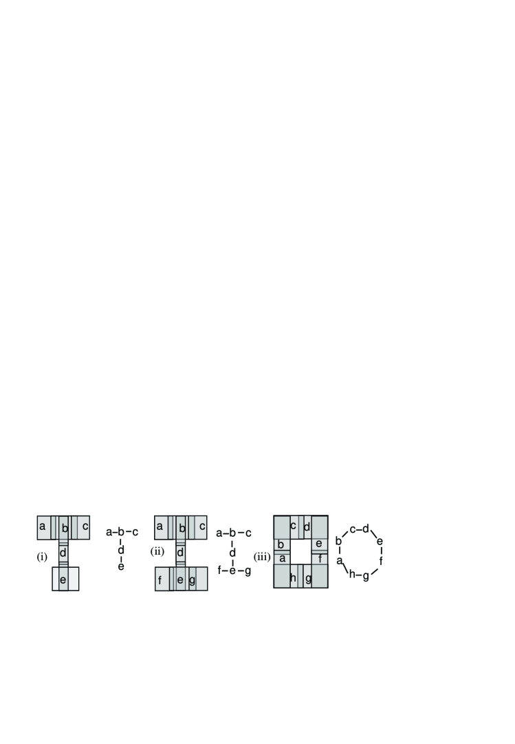
Figure 2: Three 1D environments formed by overlapping places – the darker areas show overlap between regions; to the right of each shape is the connection structure constructed by the overlaps between places, which can be distinguished by virtue of their connectivity structure.

In order to formally analyse such linear structures we can make the following definitions, which group together collections of regions to form higher level abstractions.

${\sf LinearSegment}(x)\equiv_{def}{\sf Con}(x)\wedge{\sf SumOfPlaces}(x)\wedge$
  $\forall y[[{\sf Place}(y)\wedge{\sf P}(y,x)]\rightarrow[{\sf End}(y)\vee{\sf Middle}(y)\vee{\sf Junction}(y)]]\wedge$
  $\exists!^{2}y[{\sf Place}(y)\wedge{\sf P}(y,x)\wedge[{\sf End}(y)\vee{\sf Junction}(y)]]$

${\sf End}(x)\equiv_{def}{\sf Place}(x)\wedge\exists!^{1}y[{\sf Place}(y)\wedge{\sf C}(x,y)\wedge\neg{\sf EQ}(y,x)]$

${\sf Middle}(x)\equiv_{def}{\sf Place}(x)\wedge\exists!^{2}y[{\sf Place}(y)\wedge{\sf C}(x,y)\wedge\neg{\sf EQ}(y,x)]$

${\sf Junction}(x)\equiv_{def}{\sf Place}(x)\wedge\exists^{3}y[{\sf Place}(y)\wedge{\sf C}(x,y)\wedge\neg{\sf EQ}(y,x)]$

${\sf SumOfPlaces}(x)\equiv_{def}$
  $\neg\exists y[{\sf P}(y,x)\wedge\forall z[[{\sf Place}(z)\wedge{\sf P}(z,x)]\rightarrow{\sf DC}(y,z)]]$

Thus Ends are places only connected to one other place, Middles only to two other places, and Junctions are connected to three or more other places; LinearSegments are composed of two places being either Ends or Junctions and all other places in the LinearSegment are Middles. The predicate SumOfPlaces($x$) ensures that $x$ is a region every part of which is part of some place, so that there are no “extra bits” of space which are part of $x$ but not part of some place.

These definitions achieve the desired effect in linear environments providing that no places are long enough to overlap more than one place in each direction (i.e as in fig. 3(ii)). E.g., consider fig. 3(i) – the layout is still clearly in some sense linear, but as the connection graph shows, it is not so in any very straightforward way.

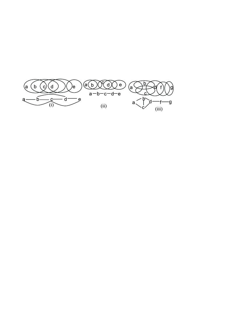
Figure 3: A linear track composed of (i) doubly overlapping places, & (ii) singly overlapping places; beneath are the connection structures formed by the overlaps. (iii): An environment with two maximal induced paths: abdfg & acdfg.

One approach to this might be to use the idea of an induced path – i.e. a sequence of nodes in a graph such that each is connected to two neighbours in the path, except for the two end nodes, and with the proviso that there are no “short cuts” (i.e. direct links) between any two nodes in the path using other edges in the graph (which would be indicated by the presence of a 3-clique). Thus in the graph in fig. 3(i), abde, ace, bce, acd, are all (maximal) induced paths. However this notion is not entirely satisfactory since it does not define a unique path for the environment (since there are two induced paths from a to e). In this case we can note that there is a unique longest induced path (abcd); of the others, ace has the same start and end nodes, and the other two each have an end in common with the longest. None are disjoint. We also note that all the nodes in the non longest induced paths are within one edge of a node on the longest induced path (i.e. c is directly linked to a,b,d and e). It is not guaranteed that there is a unique longest induced path – either because there are two entirely disjoint such paths, or because there are alternatives with common nodes – e.g. see fig. 3(iii). We thus propose the following definition for what we will call quasi linear segments.

Figure 4: A configuration in which by considering place trails from than two places simultaneously, a refined map can be obtained.

${\sf QuasiLin}(x)\equiv_{def}$
  $\exists w[{\sf P}(w,x)\wedge{\sf InducedPath}(w)\wedge{\sf SumofPlaces}(x)\wedge$
    $\forall y[[{\sf P}(y,x-w)\wedge{\sf Place}(y)]\rightarrow{\sf C}(y,w)]]$

${\sf InducedPath}(w)\equiv_{def}$
  ${\sf SumOfPlaces}(w)\wedge{\sf Con}(w)\wedge\neg\exists v[{\sf 3Clique}(v)\wedge{\sf P}(v,w)]\wedge$
  $\exists(s,x,y,z)[{\sf Place}(x)\wedge{\sf Place}(y)\wedge\neg{\sf EQ}(x,y)\wedge{\sf Place}(s)\wedge{\sf P}(s,z)\wedge$
  ${\sf EQ}(w,x+y+z)\wedge\forall u[[{\sf Place}(u)\wedge{\sf P}(u,z)]\rightarrow\neg{\sf Con}(w-u)]]$

${\sf 3Clique}(w)\equiv_{def}\exists(x,y,z)[$
  ${\sf Place}(x)\wedge{\sf Place}(y)\wedge{\sf Place}(z)\wedge{\sf EQ}(w,x+y+z)\wedge\neg{\sf EQ}(x,y)\wedge$
    $\neg{\sf EQ}(x,z)\wedge\neg{\sf EQ}(y,z)\wedge{\sf C}(x,y)\wedge{\sf C}(x,z)\wedge{\sf C}(z,y)]$

Returning to fig. 3(i), ${\sf QuasiLin}$(a+b+c+d+e) is true since it has at least one induced path in it, and all the other places in it are directly connected to a place in that induced path. Exactly what definition of “linearity” might be appropriate in a particular domain will depend on what is required or suitable for the application. E.g., ${\sf QuasiLin}(x)$ will be true if $x$ is the union of a simple path of length $m$ and a clique of size $n$ s.t. exactly two nodes are in common between the clique and the simple path. It would be straightforward to eliminate this case, or to allow only cliques of up to a size $m$ to occur within a quaslinear path.

Another important grouping of places are “open spaces” which are likely to be identified by clusters of many places, though not necessarily in the form of a clique (though they may well contain cliques). Having identified cliques, and linear segments, a natural step would be to replace these by “super nodes”, and then continue analysing the environment at this more abstract level. Indeed, there are already existing approaches to analysing and drawing graphs which take this approach, e.g. muller ; Friedrich . E.g., “open spaces” may frequently be represented as cliques of cliques.

One other aspect of connectivity analysis not so far mentioned explicitly is determining whether there are cycles in the environment (caused by circular structures in a linear environment, or by obstacles in an open environment). A graph theoretic approach to this would be to look for chordless cycles, i.e. circular induced paths of length at least four. As a trivial example of this, consider fig. 2(ii); in practice this approach is likely to require refinement to properly capture the required notion.

III Variants of the mapping task

In this section we consider a number of variants of the basic mapping task and how they might be achieved.

Computing Connectivity Mereologically: The approach outlined above shows how we can compute connection information from knowledge that the agent is simultaneously At two places. This gives rise to binary connectedness information, and thence (in RCC-5) the knowledge that particular pairs of places partially overlap (PO). It is not possible from the connection structure though to infer that any triple (quadruple…) of places overlap, even though this information might in fact be readily apparent in the place trail (indicated by an agent being simultaneously at three (four…) places). We could therefore compute a more fine grained representation, in which we explicitly represent those intersections of places which are known to exist, and similarly those relative complements of places known to exist. E.g. from the place trail: At(t1,a), At(t2,a), At(t2,b), At(t3,a), At(t3,b), At(t3,c), At(t4,b), At(t4,c), At(t5,b), At(t5,c), At(t5,d), At(t6,d), using pairwise connections, as in §II, then a connection structure as in fig. 4(i) would be computed. Not knowing about which subregions can actually exist, it would be reasonable to produce a map such as in fig. 4(ii). However, by inspecting the above place trail, we can infer that the regions a–b–c–d, a+b–c–d, a+b+c–d, b+c-a–b, b+c+d–a, and d–a–b–c all exist, but there is no evidence to support the existence of any of the other five Boolean combinations of the four places, a, b, c, d which exist in fig. 4(ii). Thus we can build a simplified map as in fig. 4(iii), in which these regions do not exist (indicated by shading).

Partial information: It is believed that PCs form a cover for the environment the rat has explored, i.e. wherever the rat is, at least one PC will be firing. However for the SRE, an external observer is receiving signals from a set of electrodes, and only a subset of the PCs will actually be recorded and thus only partial information about the set of places active at any time. At some times, there may be no active PCs being recorded, and thus there will be “temporal gaps”. The question is, what can we say about the nature of the environment given only such partial information? In the wifi domain, presumably full information would always be available; there might still be temporal gaps, because no base station is in range, but that is different to not being able to detect a base station which is in range. One might want to regard the union of all locations where there is no base station in range as a $k+1$st place. The discussion below concerns domains where there is only partial information. First we define the notion of a temporal gap:

${\sf Gap}(t_{1},t_{2})\equiv_{def}\exists(x_{1},x_{2})[{\sf At}(t_{1},x_{1})\wedge{\sf At}(t_{2},x_{2})\wedge$
  $\forall(t_{3},x_{3})[[t_{1}<t_{3}\wedge t_{3}<t_{2}]\rightarrow\neg{\sf At}(t_{3},x_{3})]$

We can now write a rule which allows us to infer that the agent must be at at least one place during a gap, and that these places form a connected region which is itself connected to all the places where the agent is at at $t_{1}$ and $t_{2}$.

$\forall(t_{1},t_{2},x_{1},x_{2})[[{\sf Gap}(t_{1},t_{2})\wedge{\sf At}(t_{1},x_{1})\wedge{\sf At}(t_{2},x_{2})]\rightarrow\\ \indent\exists x_{3}[{\sf SumOfPlaces}(x_{3})\wedge{\sf C}(x_{1},x_{3})\wedge{\sf C}(x_{2},x_{3})\wedge{\sf Con}(x_{3})]]$

There might be more than one path $x_{3}$ linking the places at $t_{1}$ and $t_{2}$, however, we cannot infer this without evidence (such as metric information about speed and distance travelled, but we do not consider such possibilities here).

There is (at least) a second way in which the underlying place information might be partial. We made the explicit assumption (in §II) that time is sufficiently fine grained that no place transitions are missed. If this is not the case (because the speed of the agent is fast with respect to the recording granularity), then gaps may occur even if there are no missing place sensors. In this case we would need a modified version of the rule above, since it may be that no new places need to be inferred to fill in the gap, but rather that at least one of the places at time $t_{1}$ directly connects with at least one of the places at time $t_{2}$. Some form of non monotonic reasoning is likely to be needed in general for reasoning in the presence of such kinds of partial knowledge, in order to perform a domain closure, or to minimize the number of places assumed to exist (as in the spatial semantic hierarchy discussed in §1).

IV Final Comments

We have discussed the problem of computing topological maps from knowledge of place trails, a task applicable at least in two identified domains. There are many ways in which this work could be extended. E.g. we could consider how to turn the symbolic topological representations into a graphic visualisation automatically. Of course any such depiction will inevitably have metric qualities, but these must be ignored when interpreting the visualization. Any qualitative spatial description will always have many metric realizations. One approach is to diagrammatic reasoning techniques (e.g. howse2 ) on visualising Euler diagrams.

We have already conducted some experimental work with artificial data and are currently collecting real data and will then evaluate the ideas sketched here, and refine them as appropriate. We may also consider other variants of the problem, e.g. scenarios with multiple agents (where the At predicate has a third argument indicating the agent).

References

- (1) J O’Keefe & L Nadel, The Hippocampus as a cognitive map, London, Oxford, (1978)
- (2) Yu. Dabaghian, A G Cohn, & L Frank, Topological coding in hippocampus, http://lanl.arxiv.org/abs/q-bio.OT/0702052
- (3) Ocana, M, Bergasa, L M, Sotelo, M A, Flores, R, Lopez, E & Barea, R, Training Method Improvements of a WiFi Navigation System Based on POMDP, IEEE/RSJ Int. Conf. on Intelligent Robots and Systems, 2006.
- (4) Kamakaris, T & Nickerson J V, Connectivity Maps: Measurements and Applications, Proc. 38th An. Hawaii international Conference on System Sciences (Hicss’05) - Track 9 - Volume 09, IEEE, 2005
- (5) A G Cohn & J Renz, Qualitative Spatial Representation and Reasoning, in V. Lifschitz, F. van Harmelen, F. Porter, Editors, Handbook of Knowledge Representation . Ch. 13, Elsevier 2007 (to appear)
- (6) E Remolina & B Kuipers, Towards a general theory of topological maps, Art. Intell. 152: 47-104, 2004
- (7) K Jeffery, J Donnett, N Burgess & J O’Keefe, Directional control of the orientation of hippocampal place fields, Exp. Brain Res., 117, pp. 131-142, 1997.
- (8) Hoang-Oanh Le, Van Bang Le, & H Mueller, Splitting a graph into disjoint induced paths or cycles, Disc. App. Maths 131 (2003) 199-212.
- (9) Friedrich, C & Schreiber, F, Flexible layering in hierarchical drawings with nodes of arbitrary size, Proc. 27th Australasian Conf. on Computer Science, 2004
- (10) Flower J & Howse J, Generating Euler Diagrams, Proc. Diagrams 2002, Springer Verlag, 61-75
- (11) M Milford, R Schulz, D Prasser, G Wyeth & J Wiles, Learning spatial concepts from RatSLAM representations, Robotics and Autonomous Systems, Vol 55(5), From Sensors to Human Spatial Concepts, 3 2007, pp 403-410