Spin-orbit coupling in bulk GaAs

Abstract

We study the spin-orbit coupling in the whole Brillouin zone for GaAs using both the $sp^{3}s^{\ast}d^{5}$ and $sp^{3}s^{\ast}$ nearest-neighbor tight-binding models. In the $\Gamma$-valley, the spin splitting obtained is in good agreement with experimental data. We then further explicitly present the coefficients of the spin splitting in GaAs $L$ and $X$ valleys. These results are important to the realization of spintronic device and the investigation of spin dynamics far away from equilibrium.

, ,

1 Introduction

Spin-orbit coupling (SOC) is the key ingredient to the semiconductor spintronic devices [1, 2]. Most of the proposed schemes of electrical generation, manipulation and detection of electron spin rely on it. Complete understanding of the SOC is therefore of great importance. In the bulk zinc-blende-type semiconductor such as GaAs, it is well known that near the center of Brillouin zone the zero field splitting caused by the SOC depends cubically on the wave-vector $k$ due to the bulk inversion asymmetry [3, 4] or linearly due to the structure inversion asymmetry [5, 6]. There are few investigations of the SOC for the states away from the band edge. The ab initio band structure calculation [7], diagonalizing of truncated $\mathbf{k}\cdot\mathbf{p}$ Hamiltonian [7] or nearest-neighbor tight-binding (TB) model including the SOC [8, 9] have been performed to obtain the spin-orbit splitting outside of the Brillouin zone center. For the states near other high symmetry points such as the $L$ and $X$ points, one can get the form of the splitting from the symmetry property [10], whereas the actual coefficients need to be further calculated. Recently the splitting of the $L$-valley in bulk GaSb and GaSb/AlSb quantum wells were calculated using an $sp^{3}s^{\ast}d^{5}$ nearest-neighbor TB model including the SOC [8]. It is shown that the splitting in GaSb $L$-valley exceeds 10 meV, an order of magnitude larger than the typical value in the $\Gamma$-valley. For GaAs the corresponding data are still not available.

The lack of quantitative information of the SOC outside the Brillouin center is not crucial to the development of spintronics at the present stage, since the electrons in most of the study locate at the bottom of the $\Gamma$-valley. However, in real situation, the devices usually work under high electric field which can drive the electrons to the states far away from $\Gamma$ point, or even further to other valleys such as $L$- and/or $X$-valleys. Therefore for the realization of the spintronic devices, the SOC in the whole Brillouin zone is essential. In the previous works on high field spin transport in GaAs [11, 12], the coefficient of spin splitting in high valleys are approximated by other material such as GaSb due to the lack of the corresponding data for GaAs. In this report we present the spin splitting of GaAs for the whole lowest conduction band. Especially, we calculate the the coefficients of spin splitting in $L$- and $X$- valleys.

2 Calculation and Results

Our calculations are performed in $sp^{3}s^{*}$ and $sp^{3}s^{*}d^{5}$ nearest-neighbor TB models with the SOC. This method has been proven to be an effective approach in band structure calculations [9, 13, 14, 15, 16, 17, 18]. The parameters we use are adopted from the published literate [9, 13, 14, 15, 16, 17, 18]. The original parameter sets have been optimized to fit the experimental data, such as the band edge and the effective mass. With the comparison to the experimental data, the spin splitting near the $\Gamma$-point is calculated as the benchmark of the suitability of these parameters for calculating the spin splitting.

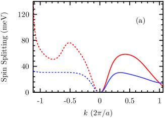
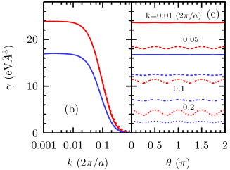
Figure 1: (Color Online) (a) Spin splitting in $\Gamma$-valley for different momentum along $\Gamma$-$K$ (solid curves) and $\Gamma$-$W$ (dashed curves) directions; (b) The corresponding SOC coefficient $\gamma$ vs. momentum along $\Gamma$-$K$ (solid curves) and $\Gamma$-$W$ (dashed curves) directions; (c) $\gamma$ vs. angle of the momentum with different amplitudes. Solid curves: $k=0.01$; Dashed curves: $k=0.05$; Chain curves: $k=0.1$; Dotted curves: $k=0.2$ $(2\pi/a)$, respectively. Red/Blue curves are the results from the $sp^{3}s^{\ast}d^{5}$/$sp^{3}s^{\ast}$ model.

In Fig. 1 we show the spin splitting around $\Gamma$ point for different momentums. In the figure the parameter sets are chosen from Refs. [15] and [9] for $sp^{3}s^{\ast}$ and $sp^{3}s^{\ast}d^{5}$ respectively. One can see from the figure that for small momentum the splittings calculated from $sp^{3}s^{\ast}$ and $sp^{3}d^{5}s^{\ast}$ approaches both increase with the momentum. When the momentum becomes large, the splitting is no longer a monotonic. The splittings along different directions have different behaviors. For the states near the $\Gamma$-point, the splitting can be described by $\gamma\mathbf{\Omega}(\mathbf{k})\cdot\mbox{\boldmath$\sigma$\unboldmath}$ with $\sigma$ being the Pauli matrices. In the coordinate system of $\hat{x}=[100]$, $\hat{y}=[010]$ and $\hat{z}=[001]$,

$$\gamma\mathbf{\Omega}(\mathbf{k})=\gamma(k_{x}(k_{y}^{2}-k_{z}^{2}),k_{y}(k_{z}^{2}-k_{x}^{2}),k_{z}(k_{x}^{2}-k_{y}^{2})).$$ (1)

This gives rise to a splitting that varies cubically in $k$, i.e., $\Delta E\sim\gamma k^{3}$. The splitting along different directions are different. In the $x$-$y$ plane, the splitting is $\Delta E=\gamma k^{3}|\sin(2\theta)|$ where $\theta$ is the angle between the momentum and $(100)$-axis. The exact value of $\gamma$ is still in debate. Different approaches give various values range from 8.5 to 34.5 eV$\cdot$ų. Overviews of these results are nicely listed in Refs. [19, 20]. Theoretical calculations based on different approaches give quite different values. There are two kinds of experiments that can measure $\gamma$ value. One is through the direct measurement of the splitting using Raman scattering. Experiments based on this approach show that $\gamma$ is about 23.5 eV$\cdot$ų in wide GaAs quantum well [21]. In asymmetric GaAs/AlGaAs heterostructure/quantum well, $\gamma$ is about 16.5 or 11.0 eV$\cdot$ų [22, 23]. The other kind of measurement is through spin relaxation time or magneto-conductance. This kind of measurement is indirect since it depends on how to qualitatively calculate the spin relaxation time or magneto-conductance. Earlier works of this kind estimate that $\gamma$ is about 20-30 eV$\cdot$ų [24, 25, 26]. Recent calculation based on fully microscopic approach reveals that the experiments in two-dimensional (2D) system can be explained by using much smaller $\gamma$ value [27]. In our calculation, value of this coefficient is calculated as $\gamma(\mathbf{k})=\Delta E/(2|\Omega(\mathbf{k})|)$. The results for different momentums are shown in Fig. 1(b) and (c). One can see from the figure that for $k<0.04\pi/a$, $\gamma$ is almost a constant that is independent on magnitude and the angle of momentum. For the parameters we use, $sp^{3}s^{\ast}$ and $sp^{3}s^{\ast}d^{5}$ give $\gamma=17.0$ and $23.9$ eV$\cdot$ų near the $\Gamma$-point, respectively. Both are close to the experimental data from Raman scattering. This good agreement between the theoretical result and the experimental data shows that the parameters we use can be applied to study the spin splitting for whole Brillouin zone. One can see from the figure that both models predict that the value of $\gamma$ decreases with the increase of momentum. Moreover, angle dependence of $\gamma$ becomes remarkable for large momentum. Thus $\gamma$ is no longer a constant for large momentum. Practically the SOC described by Eq. (1) with constant $\gamma$ is a good approximation for the state not far away from equilibrium since even for high-carrier-density samples the value of $\gamma$ at Fermi surface is only a few percents smaller than the value at $k=0$. However, when electrons are driven far away from the $\Gamma$ point, Eq. (1) is expected to over-estimate the SOC.

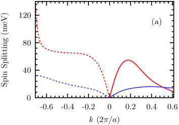
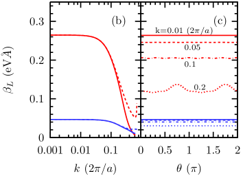
Figure 2: (Color Online) (a) Spin splitting in $L$-valley for different momentums along $L$-$K$ (solid curves) and $L$-$W$ (dashed curves) directions; (b) The corresponding SOC coefficients $\beta_{L}$ vs. momentum along $L$-$K$ (solid curves) and $L$-$W$ (dashed curves) directions; (c) $\beta_{L}$ vs. angle of the momentum with different amplitudes. Solid curves: $k=0.01$; Dashed curves: $k=0.05$; Chain curves: $k=0.1$; Dotted curves: $k=0.2$ $(2\pi/a)$, respectively. Red/Blue curves are the results from the $sp^{3}s^{\ast}d^{5}$/$sp^{3}s^{\ast}$ model.

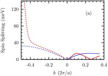
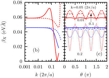
Figure 3: (Color Online) (a) Spin splitting in $X$-valley for different momentums along $X$-$K$ (solid curves) and $X$-$W$ (dashed curves) directions; (b) The corresponding SOC coefficient $\beta_{X}$ vs. momentum along $X$-$K$ (solid curves) and $X$-$W$ (dashed curves) directions; (c) $\beta_{X}$ vs. angle of the momentum with different amplitudes. Solid curves: $k=0.01$; Dashed curves: $k=0.05$; Chain curves: $k=0.1$; Dotted curves: $k=0.2$ $(2\pi/a)$, respectively. Red/Blue curves are the results from the $sp^{3}s^{\ast}d^{5}$/$sp^{3}s^{\ast}$ model.

We now turn to the states in $L$- and $X$-valleys. The spin splittings for different momentums are plotted in Figs. 2 and 3(a) respectively. One can see from the figures that, for the same amount of momentum variation from the valley bottom, the spin splitting in $L$/$X$-valley is much larger than that in $\Gamma$-valley. For the states near the $X$-point, the SOC is in the form [10], $\beta_{X}\mathbf{\Omega}_{X}(\mathbf{k})\cdot\mbox{\boldmath${\sigma}$\unboldmath}$ with

$$\beta_{X}\mathbf{\Omega}_{X}(\mathbf{k})=\beta_{X}(k_{x},-k_{y},0)\ .$$ (2)

Near the $L$-valley bottom, the SOC reads $\beta_{L}\mathbf{\Omega}_{L}(\mathbf{k})\cdot\mbox{\boldmath$\sigma$\unboldmath}$. In the new coordinate system spanned by [1$\bar{1}$0] ($x^{\prime}$-axis), [11$\bar{2}$] ($y^{\prime}$-axis) and [111] ($z^{\prime}$-axis) vectors, $\mathbf{\Omega}_{L}(\mathbf{k})$ reads [10]

$$\beta_{L}\mathbf{\Omega}_{L}(\mathbf{k})=\beta_{L}(k_{y}^{\prime},-k_{x}^{\prime},0)\ .$$ (3)

In the above two equations, $\mathbf{k}$ represents the momentum vector measured from $L$/$X$-valley bottom. These couplings give the splitting linear to the first order of momentum around the valley bottoms. The corresponding splitting coefficients $\beta_{L/X}=\Delta{E}(k)/2k$ for different momentum are plotted in Figs. 2(b) and 3(b) respectively. Similar to that of $\Gamma$-valley, these coefficients are constants near the valley bottoms. In the $X$-valley, the values of $\beta_{X}$ obtained from $sp^{3}s^{\ast}d^{5}$ and $sp^{3}s^{\ast}$ models are close to each other, i.e., $\beta_{X}=0.059$ and 0.046 eV$\cdot$Å, respectively. However, in the $L$-valley, $\beta_{L}$ determined from these two models are quite different. For $sp^{3}s^{\ast}d^{5}$, $\beta_{L}=0.26$ eV$\cdot$Å; while for $sp^{3}s^{\ast}$, $\beta_{L}=0.047$ eV$\cdot$Å. This profound difference implies that the $d$ orbit plays an important role in the spin splitting in the $L$-valley of the lowest conduction band. This is because the symmetry imposes a $d$-orbital component in the $L$-valley and $sp^{3}s^{\ast}d^{5}$ model can account this symmetry more accurate. It has been revealed that the inclusion of the $d$ orbit greatly improves the accuracy of the effective mass in $L$-valley [9, 28, 29, 30, 31]. Therefore, in our opinion the spin splitting determined by $sp^{3}s^{\ast}d^{5}$ model in $L$-valley is also more reliable than that by $sp^{3}s^{\ast}$ model.

3 Conclusion

In conclusion we study the SOC in the whole Brillouin zone for GaAs using both $sp^{3}s^{\ast}d^{5}$ and $sp^{3}s^{\ast}$ nearest-neighbor TB models. For the parameter sets we use, the spin splittings calculated from both models are in good agreement with experimental data in the $\Gamma$-valley. We then further explicitly present the coefficients of the spin splitting in the $L$ and $X$ valleys. These results are useful for understanding the spin dynamics far away from equilibrium.

References

- [1] S. A. Wolf, J. Supercond.: Incorporating Novel Magnetism 13 (2000) 195.
- [2] I. Žutić, J. Fabian, S. D. Sarma, Rev. Mod. Phys. 76 (2004) 323.
- [3] M. I. D’yakonov, V. I. Perel’, Zh. Eksp. Teor. Fiz. 60 (1971) 1954, [Sov. Phys.-JETP 33, 1053 (1971)].
- [4] M. I. D’yakonov, V. I. Perel’, Fiz. Tverd. Tela 13 (1971) 3581, [Sov. Phys. Solid State 13, 3023 (1972)].
- [5] Y. A. Bychkov, E. I. Rashba, J. Phys. C 17 (1984) 6039.
- [6] Y. A. Bychkov, E. I. Rashba, Pis’ma Zh. Eksp. Teor. Fiz. 39 (1984) 66.
- [7] M. Cardona, N. E. Christensen, G. Fasol, Phys. Rev. B 38 (1988) 1806.
- [8] J.-M. Jancu, R. Scholz, G. C. L. Rocca, E. A. de Andrada e Silva, P. Voisin, Phys. Rev. B 70 (2004) 121306(R).
- [9] J.-M. Jancu, R. Scholz, F. Beltram, F. Bassani, Phys. Rev. B 57 (1998) 6493.
- [10] E. L. Ivchenko, G. E. Pikus, Superlattices and Other Heterostructures, Springer, Berlin, 1995.
- [11] S. Saikin, M. Shen, M.-C. Cheng, J. Phys.: Condens. Matter 18 (2006) 1535.
- [12] M. Shen, S. Saikin, M.-C. Cheng, V. Privman, Mathematics and Computers in Simulation 65 (2004) 351.
- [13] P. Vogl, H. P. Hjalmarson, J. D. Dow, J. Phys. Chem. Solids 44 (1983) 365.
- [14] P. V. Santos, M. Willatzen, M. Cardona, A. Cantarero, Phys. Rev. B 51 (1995) 5121.
- [15] J. Klimeck, R. C. Bowen, T. B. Boykin, T. A. Cwik, Superlattices and Microstructures 27 (2000) 519.
- [16] T. B. Boykin, G. Klimeck, R. C. Bowen, R. Lake, Phys. Rev. B 56 (1997) 4102.
- [17] T. B. Boykin, G. Klimeck, R. C. Bowen, F. Oyafuso, Phys. Rev. B 66 (2002) 125207.
- [18] J. G. Dïaz, G. W. Bryant, Phys. Rev. B 73 (2006) 075329.
- [19] J. J. Krich, B. I. Halperin, Phys. Rev. Lett. 98 (2007) 226802.
- [20] A. N. Chantis, M. van Schilfgaarde, T. Kotani, Phys. Rev. Lett. 98 (2006) 086405.
- [21] D. Richards, B. Jusserand, H. Peric, B. Etienne, Phys. Rev. B 47 (1993) 16028.
- [22] B. Jusserand, D. Richards, G. Allan, C. Priester, B. Etienne, Phys. Rev. B 51 (1995) 4707.
- [23] D. Richards, B. Jusserand, G. Allan, C. Priester, B. Etienne, Solid-State Electron. 40 (1996) 127.
- [24] V. I. Marushak, T. V. Lagunova, M. N. Seepanova, A. N. Titkov, Fiz. Tverd. Tela 25 (1983) 2140.
- [25] A. G. Aronov, G. E. Pikus, A. N. Titkov, Zh. Eksp. Teor. Fiz. 84 (1983) 1170, [Sov. Phys.-JETP 57, 680 (1983)].
- [26] J. B. Miller, D. M. Zumbühl, C. M. Marcus, Y. B. Lyanda-Geller, D. Goldhaber-Gordon, K. Campman, A. C. Gossard, Phys. Rev. Lett. 90 (2003) 076807.
- [27] J. Zhou, J. L. Cheng, M. W. Wu, Phys. Rev. B 75 (2007) 045305.
- [28] S. B. Singh, C. A. Singh, Am. J. Phys. 57 (1989) 894.
- [29] Y.-C. Chang, D. E. Aspnes, Phys. Rev. B 41 (1990) 12002.
- [30] S. L. Richardson, M. L. Cohen, S. G. Louie, J. R. Chelikowsky, Phys. Rev. B 33 (1986) 1177.
- [31] P. Boguslawsky, I. Gorczyca, Semicond. Sci. Technol. 9 (1994) 2169.