QuanTree and QuanLin,
Two Special Purpose
Quantum Compilers

Abstract

This paper introduces QuanTree v1.1 and QuanLin v1.1, two Java applications available for free. (Source code included in the distribution.) Each application compiles a different type of input quantum evolution operator. The applications output a quantum circuit that is approximately equal to the input evolution operator. QuanTree compiles an input evolution operator whose Hamiltonian is proportional to the incidence matrix of a balanced, binary tree graph. QuanLin compiles an input evolution operator whose Hamiltonian is proportional to the incidence matrix of a line (open string) graph. Both applications also output an error, defined as the distance in the Frobenius norm between the input evolution operator and the output quantum circuit.

1 Introduction

We say a unitary operator acting on a set of qubits has been compiled if it has been expressed as a SEO (sequence of elementary operations, like CNOTs and single-qubit operations). SEO’s are often represented as quantum circuits.

There exist software (quantum compilers) like Qubiter[1] for compiling arbitrary unitary operators (operators that have no a priori known structure). This paper introduces two special purpose quantum compilers, QuanTree and QuanLin. They are special purpose in the sense that they can only compile unitary operators that have a very definite, special structure.

QuanTree v1.0 and QuanLin v1.1 are two Java applications, available[2] for free. (Source code included in the distribution.) Each application compiles a different kind of input quantum evolution operator. The applications output a quantum circuit that is approximately equal to the input evolution operator. QuanTree compiles an input evolution operator whose Hamiltonian is proportional to the incidence matrix of a balanced, binary tree graph. QuanLin compiles an input evolution operator whose Hamiltonian is proportional to the incidence matrix of a line (open string) graph. Both applications also output an error, defined as the distance in the Frobenius norm between the input evolution operator and the output quantum circuit.

Recently, Farhi-Goldstone-Gutmann (FGG) wrote a paper[3] that proposes a quantum algorithm for evaluating NAND formulas via a quantum walk over a tree graph connected to a line (“runway”) graph. Their paper has inspired a flurry of papers expanding on their ideas. Among these papers is one[4] written by me, which provides all the theoretical underpinnings of QuanTree and QuanLin. Please refer to Ref.[4] and the source code of QuanTree and QuanLin if you have any technical questions that are no addressed here. To get a quantum circuit for the FGG algorithm requires first finding a quantum circuit for the evolution operators of a tree and line graph, which is what QuanTree and QuanLin do. A future paper will combine QuanTree and QuanLin software to give a quantum circuit for the full FGG algorithm.

The standard definition of the evolution operator in Quantum Mechanics is $U=e^{-itH}$, where $t$ is time and $H$ is a Hamiltonian. Throughout this paper, we will set $t=-1$ so $U=e^{iH}$. If $H$ is proportional to a coupling constant $g$, reference to time can be restored easily by replacing the symbol $g$ by $-tg$, and the symbol $H$ by $-tH$.

2 QuanTree

2.1 Input Evolution Operator

A binary tree with ${\Lambda}+1$ levels has $1+2+2^{2}+\ldots 2^{{\Lambda}}=2^{{\Lambda}+1}-1$ nodes (a.k.a. as states). To reach ${N_{S}}=2^{{\Lambda}+1}$ states, we add an extra “dead” or “dud” node, labelled with the letter “$d$”. This $d$ node is not connected to any other node in the graph. If we include this dud node, then the number of leaves ${N_{lvs}}$ is exactly half the number of nodes: ${N_{lvs}}=\frac{1}{2}2^{{\Lambda}+1}=2^{\Lambda}$. We will often use ${N_{B}}$ for the number of bits and ${N_{S}}=2^{N_{B}}$ for the number of states. Therefore, ${N_{B}}={\Lambda}+1$. For example, Fig.1 shows a binary-tree graph with ${\Lambda}=2$ and ${N_{B}}=3$. It has ${N_{S}}=2^{{\Lambda}+1}$=8 nodes, labelled $d,1,2,\ldots,7$, half of which ($4,5,6,7$) are leaves.

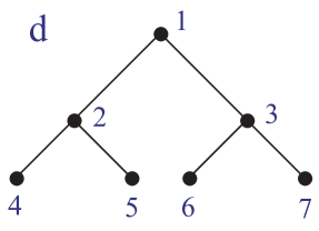
Figure 1: Binary tree with 8 nodes

The Hamiltonian for transitions along the edges of the graph Fig.1 is:

$$H_{tree}=g\begin{array}[]{c|c|c|c|c|c|c|c|c|}&{\scriptscriptstyle d}&{\scriptscriptstyle 1}&{\scriptscriptstyle 2}&{\scriptscriptstyle 3}&{\scriptscriptstyle 4}&{\scriptscriptstyle 5}&{\scriptscriptstyle 6}&{\scriptscriptstyle 7}\\ \hline\cr{\scriptscriptstyle d}&&&&&&&&\\ \hline\cr{\scriptscriptstyle 1}&&&1&1&&&&\\ \hline\cr{\scriptscriptstyle 2}&&1&&&1&1&&\\ \hline\cr{\scriptscriptstyle 3}&&1&&&&&1&1\\ \hline\cr{\scriptscriptstyle 4}&&&1&&&&&\\ \hline\cr{\scriptscriptstyle 5}&&&1&&&&&\\ \hline\cr{\scriptscriptstyle 6}&&&&1&&&&\\ \hline\cr{\scriptscriptstyle 7}&&&&1&&&&\\ \hline\cr\end{array}\;,$$ (1)

where $g$ is a real number that we will call the coupling constant. In Eq.(1), empty matrix entries represent zero.

For ${N_{B}}=3$ qubits (i.e., $2^{N_{B}}=8$ states), the input evolution operator for QuanTree is $U=e^{iH_{tree}}$, where $H_{tree}$ is given by Eq.(1). It is easy to generalize Fig.1 and Eq.(1) to arbitrary ${N_{B}}$. QuanTree can compile $e^{iH_{tree}}$ for ${N_{B}}\in\{2,3,4,\ldots\}$.

For $r=1,2,3,\ldots$, if $U=L_{r}(g)+{\cal O}(g^{r+1})$, we say $L_{r}(g)$ approximates (or is an approximant) of order $r$ for $U$.

Given an approximant $L_{r}(g)+{\cal O}(g^{r+1})$ of $U$, and some ${N_{T}}=1,2,3\,\ldots$, one can approximate $U$ by $\left(L_{r}(\frac{g}{{N_{T}}})\right)^{N_{T}}+{\cal O}(\frac{g^{r+1}}{{N_{T}}^{r}})$. We will refer to this as Trotter’s trick, and to ${N_{T}}$ as the number of trots.

For ${N_{T}}=1$, QuanTree approximates $e^{iH_{tree}}$ with an approximant of order 3 that is derived in Ref.[4]. Thus, for ${N_{T}}=1$, the error is ${\cal O}(g^{4})$. For ${N_{T}}>1$, the error is ${\cal O}(\frac{g^{4}}{{N_{T}}^{3}})$.

2.2 The Control Panel

Fig.2 shows the Control Panel for QuanTree. This is the main and only window of the application. This window is open if and only if the application is running.

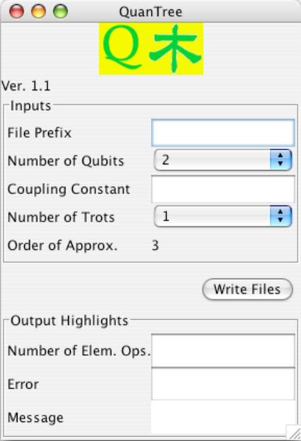
Figure 2: Control Panel of QuanTree

The Control Panel allows you to enter the following inputs:

File Prefix:

Prefix to the 3 output files that are written when you press the Write Files button. For example, if you insert test in this text field, the following 3 files will be written:

• test_qtree_log.txt (See Fig.3)

• test_qtree_eng.txt (See Fig.4)

• test_qtree_pic.txt (See Fig.5)

Number of Qubits:

The parameter ${N_{B}}=2,3,4,\ldots$ defined above.

Coupling Constant:

The parameter $g\in{\mathbb{R}}$ defined above.

Number of Trots:

The parameter ${N_{T}}=1,2,3,\ldots$ defined above.

The Control Panel displays the following outputs:

Number of Elementary Operations:

The number of elementary operations in the output quantum circuit. If there are no LOOPs, this is the number of lines in the English File (see Sec. 2.3.2), which equals the number of lines in the Picture File (see Sec. 2.3.3). When there are LOOPs, the “LOOP k REPS:${N_{T}}$” and “NEXT k” lines are not counted, whereas the lines between “LOOP k REPS:${N_{T}}$” and “NEXT k” are counted ${N_{T}}$ times.

Error:

The distance in the Frobenius norm between the input evolution operator and the output quantum circuit (i.e., the SEO given in the English File). For a nice review of matrix norms, see Ref.[5]. For any matrix $A\in{\mathbb{C}}^{n\times n}$, its Frobenius norm is defined as $\|A\|_{F}=\sqrt{\sum_{j,k}A_{j,k}A^{*}_{j,k}}$. Another common matrix norm is the 2-norm. The 2-norm $\|A\|_{2}$ of $A$ equals the largest singular value of $A$. The Frobenius and 2-norm of $A$ are related by[5]: $\|A\|_{2}\leq\|A\|_{F}\leq\sqrt{2}\|A\|_{2}$. Since the approximant used by QuanTree is of order 3, if $\epsilon$ denotes the error, then $\epsilon(g)\approx Kg^{4}$, for some $K\in{\mathbb{R}}$ and $|g|<<1$. Thus,

$$\frac{\log(\epsilon(g_{2})/\epsilon(g_{1}))}{\log(g_{2}/g_{1})}\approx 4\;.$$ (2)

For example, with ${N_{B}}=4$ and ${N_{T}}=1$, QuanTree gives $\epsilon(0.05)=1.383\times 10^{-5}$ and $\epsilon(0.06)=2.923\times 10^{-5}$, which gives $\log(\epsilon_{2}/\epsilon_{1})/\log(g_{2}/g_{1})=4.11$.

Message:

A message appears in this text field if you press Write Files with a bad input. The message tries to explain the mistake in the input.

2.3 Output Files

Figs.3, 4, 5, were all generated in a single run of QuanTree (by pressing the Write Files button just once). They are examples of what we call the Log File, English File, and Picture File, respectively, of QuanTree. Next we explain the contents of each of these output files.

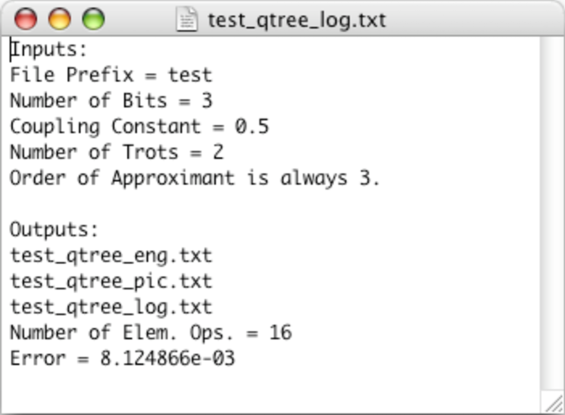
Figure 3: Log File generated by QuanTree

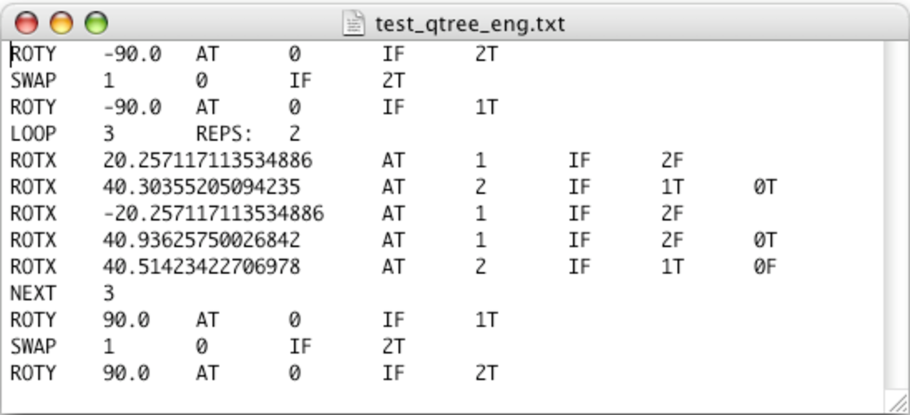
Figure 4: English File generated by QuanTree

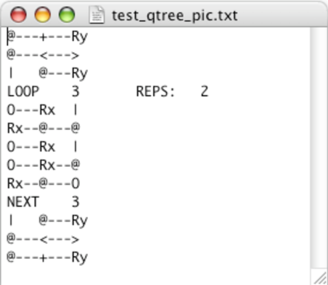
Figure 5: Picture File generated by QuanTree

2.3.1 Log File

Fig.3 is an example a Log File. The Log File records all the information found in the Control Panel.

2.3.2 English File

Fig.4 is an example of an English File. The English File completely specifies the output SEO. It does so “in English”, thus its name. Each line represents one elementary operation, and time increases as we move downwards.

In general, an English File obeys the following rules:

• Time grows as we move down the file.

• Each row corresponds to one elementary operation. Each row starts with 4 letters that indicate the type of elementary operation.

• For a one-bit operation acting on a “target bit” $\alpha$, the target bit $\alpha$ is given after the word AT.

• If the one-bit operation is controlled, then the controls are indicated after the word IF. T and F stand for true and false, respectively. $\alpha$T stands for a control $n(\alpha)$ at bit $\alpha$. $\alpha$F stands for a control ${\overline{n}}(\alpha)$ at bit $\alpha$.

• “LOOP k REPS:${N_{T}}$” and “NEXT k” mark the beginning and end of ${N_{T}}$ Trotter iterations. k labels the loop. k also equals the line-count number (first line is 0) of the line “LOOP k REPS:${N_{T}}$” in the English file.

• SWAP $\alpha$ $\beta$ stands for the swap(exchange) operator $E(\alpha,\beta)$ that swaps bits $\alpha$ and $\beta$.

• PHAS stands for a controlled one-bit gate, where the one-bit gate consists of $diag(1,1)$ times an angle (“phase”).

• P0PH stands for a controlled one-bit gate, where the one-bit gate consists of $P_{0}={\overline{n}}()$ times an angle (“phase”). P1PH stands for a controlled one-bit gate, where the one-bit gate consists of $P_{1}=n()$ times an angle (“phase”).

• SIGX, SIGY, SIGZ, HAD2 stand for the Pauli matrices ${\sigma_{X}},{\sigma_{Y}},{\sigma_{Z}}$ and the one-bit Hadamard matrix $H$.

• ROTX, ROTY, ROTZ, ROTN stand for rotations with rotation axes in the directions: $x$, $y$, $z$, and an arbitrary direction $n$, respectively.

Here is a list of examples showing how to translate the mathematical notation used in Ref.[4] into the English File language:

Mathematical language	English File language
Loop called 5 with 2 repetitions	LOOP 5 REPS: 2
Next iteration of loop called 5	NEXT 5
$E(1,0)^{{\overline{n}}(3)n(2)}$	SWAP 1 0 IF 3F 2T
$e^{i42.7{\overline{n}}(3)n(2)}$	PHAS 42.7 IF 3F 2T
$e^{i42.7{\overline{n}}(3)n(2)}$	P0PH 42.7 AT 3 IF 2T
$e^{i42.7n(3)n(2)}$	P1PH 42.7 AT 3 IF 2T
${\sigma_{X}}(1)^{{\overline{n}}(3)n(2)}$	SIGX AT 1 IF 3F 2T
${\sigma_{Y}}(1)^{{\overline{n}}(3)n(2)}$	SIGY AT 1 IF 3F 2T
${\sigma_{Z}}(1)^{{\overline{n}}(3)n(2)}$	SIGZ AT 1 IF 3F 2T
$H(1)^{{\overline{n}}(3)n(2)}$	HAD2 AT 1 IF 3F 2T
$(e^{\frac{i}{2}\frac{\pi}{180}23.7{\sigma_{X}}(1)})^{{\overline{n}}(3)n(2)}$	ROTX 23.7 AT 1 IF 3F 2T
$(e^{\frac{i}{2}\frac{\pi}{180}23.7{\sigma_{Y}}(1)})^{{\overline{n}}(3)n(2)}$	ROTY 23.7 AT 1 IF 3F 2T
$(e^{\frac{i}{2}\frac{\pi}{180}23.7{\sigma_{Z}}(1)})^{{\overline{n}}(3)n(2)}$	ROTZ 23.7 AT 1 IF 3F 2T
$(e^{\frac{i}{2}\frac{\pi}{180}[30{\sigma_{X}}(1)+40{\sigma_{Y}}(1)+11{\sigma_{Z}}(1)]})^{{\overline{n}}(3)n(2)}$	ROTN 30.0 40.0 11.0 AT 1 IF 3F 2T

2.3.3 ASCII Picture File

Fig.5 is an example of a Picture File. The Picture File partially specifies the output SEO. It gives an ASCII picture of the quantum circuit. Each line represents one elementary operation, and time increases as we move downwards. There is a one-to-one onto correspondence between the rows of the English and Picture Files.

In general, a Picture File obeys the following rules:

• Time grows as we move down the file.

• Each row corresponds to one elementary operation. Columns $1,5,9,13,\ldots$ represent qubits (or, qubit positions). We define the rightmost qubit as 0. The qubit immediately to the left of the rightmost qubit is 1, etc. For a one-bit operator acting on a “target bit” $\alpha$, one places a symbol of the operator at bit position $\alpha$.

• | represents a wire connecting the same qubit at two times.

• -represents a wire connecting different qubits at the same time.

• + represents both | and -.

• If the one-bit operation is controlled, then the controls are indicated as follows. @ at bit position $\alpha$ stands for a control $n(\alpha)$. 0 at bit position $\alpha$ stands for a control ${\overline{n}}(\alpha)$.

• “LOOP k REPS:${N_{T}}$” and “NEXT k” mark the beginning and end of ${N_{T}}$ Trotter iterations. k labels the loop. k also equals the line-count number (first line is 0) of the line “LOOP k REPS:${N_{T}}$” in the picture file.

• The swap(exchange) operator $E(\alpha,\beta)$ is represented by putting arrow heads < and > at bit positions $\alpha$ and $\beta$.

• A phase factor $e^{i\theta}$ for some angle $\theta$ is represented by placing Ph at any bit position which does not already hold a control.

• The one-bit gate $P_{0}(\alpha)={\overline{n}}(\alpha)$ times an angle is represented by putting OP at bit position $\alpha$.

• The one-bit gate $P_{1}(\alpha)=n(\alpha)$ times an angle is represented by putting @P at bit position $\alpha$.

• One-bit operations ${\sigma_{X}}(\alpha)$, ${\sigma_{Y}}(\alpha)$, ${\sigma_{Z}}(\alpha)$ and $H(\alpha)$ are represented by placing the letters X,Y,Z, H, respectively, at bit position $\alpha$.

• One-bit rotations acting on bit $\alpha$, in the $x,y,z,n$ directions, are represented by placing Rx,Ry,Rz, R, respectively, at bit position $\alpha$.

Here is a list of examples showing how to translate the mathematical notation used in Ref.[4] into the Picture File language:

Mathematical language	Picture File language
Loop called 5 with 2 repetitions	LOOP 5 REPS:2
Next iteration of loop called 5	NEXT 5
$E(1,0)^{{\overline{n}}(3)n(2)}$	0---@---<--->
$e^{i42.7{\overline{n}}(3)n(2)}$	0---@---+--Ph
$e^{i42.7{\overline{n}}(3)n(2)}$	0P--@   |   |
$e^{i42.7n(3)n(2)}$	@P--@   |   |
${\sigma_{X}}(1)^{{\overline{n}}(3)n(2)}$	0---@---X   |
${\sigma_{Y}}(1)^{{\overline{n}}(3)n(2)}$	0---@---Y   |
${\sigma_{Z}}(1)^{{\overline{n}}(3)n(2)}$	0---@---Z   |
$H(1)^{{\overline{n}}(3)n(2)}$	0---@---H   |
$(e^{\frac{i}{2}\frac{\pi}{180}23.7{\sigma_{X}}(1)})^{{\overline{n}}(3)n(2)}$	0---@---Rx  |
$(e^{\frac{i}{2}\frac{\pi}{180}23.7{\sigma_{Y}}(1)})^{{\overline{n}}(3)n(2)}$	0---@---Ry  |
$(e^{\frac{i}{2}\frac{\pi}{180}23.7{\sigma_{Z}}(1)})^{{\overline{n}}(3)n(2)}$	0---@---Rz  |
$(e^{\frac{i}{2}\frac{\pi}{180}[30{\sigma_{X}}(1)+40{\sigma_{Y}}(1)+11{\sigma_{Z}}(1)]})^{{\overline{n}}(3)n(2)}$	0---@---R   |

2.4 Behind the Scenes

Brief summary of the steps taken by QuanTree every time you press the Write Files button:

1. Generate the English and Picture Files according to the rules of Ref.[4].

2. Generate $H$. Calculate the eigenvalues and eigenvectors of $H$. Use this eigensystem to calculate $U=e^{iH}$.

3. Read the English File that was written in Step 1. Multiply out the SEO given by the English File to obtain a unitary matrix $U^{\prime}$. Calculate the error $\|U-U^{\prime}\|_{F}$.

4. Generate the Log File.

3 QuanLin

3.1 Input Evolution Operator

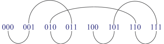
Figure 6: Line (open string) with 8 nodes

Let ${N_{B}}$ be the number of bits and ${N_{S}}=2^{N_{B}}$ the number of states. Fig.6 shows the 8 possible states for 3 bits. The states read from left to right are in increasing “decimal ordering”. These 8 states can also be ordered in “Gray code ordering”. A sequence of Gray code is one wherein two consecutive states are labelled by a binary number and these labels differ only at one bit position. In Fig.6, states connected by an edge (curved line) are consecutive in a Gray code ordering.

The Hamiltonian for transitions along the edges of the graph Fig.6 is:

$$H_{line}=g\begin{array}[]{c|c|c|c|c|c|c|c|c|}&{\scriptscriptstyle 000}&{\scriptscriptstyle 001}&{\scriptscriptstyle 010}&{\scriptscriptstyle 011}&{\scriptscriptstyle 100}&{\scriptscriptstyle 101}&{\scriptscriptstyle 110}&{\scriptscriptstyle 111}\\ \hline\cr{\scriptscriptstyle 000}&0&1&&&&&&\\ \hline\cr{\scriptscriptstyle 001}&1&0&&1&&&&\\ \hline\cr{\scriptscriptstyle 010}&&&0&1&&&1&\\ \hline\cr{\scriptscriptstyle 011}&&1&1&0&&&&\\ \hline\cr{\scriptscriptstyle 100}&&&&&0&1&&\\ \hline\cr{\scriptscriptstyle 101}&&&&&1&0&&1\\ \hline\cr{\scriptscriptstyle 110}&&&1&&&&0&1\\ \hline\cr{\scriptscriptstyle 111}&&&&&&1&1&0\\ \hline\cr\end{array}\;,$$ (3)

where $g$ is a real number that we will call the coupling constant. In Eq.(3), empty matrix entries represent zero.

For ${N_{B}}=3$ qubits (i.e., $2^{N_{B}}=8$ states), the input evolution operator for QuanLin is $U=e^{iH_{line}}$, where $H_{line}$ is given by Eq.(3). It is easy to generalize Fig.6 and Eq.(3) to arbitrary ${N_{B}}$. QuanLin can compile $e^{iH_{line}}$ for ${N_{B}}\in\{2,3,4,\ldots\}$.

For $r=1,2,3,\ldots$, if $U=L_{r}(g)+{\cal O}(g^{r+1})$, we say $L_{r}(g)$ approximates (or is an approximant) of order $r$ for $U$.

Given an approximant $L_{r}(g)+{\cal O}(g^{r+1})$ of $U$, and some ${N_{T}}=1,2,3\,\ldots$, one can approximate $U$ by $\left(L_{r}(\frac{g}{{N_{T}}})\right)^{N_{T}}+{\cal O}(\frac{g^{r+1}}{{N_{T}}^{r}})$. We will refer to this as Trotter’s trick, and to ${N_{T}}$ as the number of trots.

For ${N_{T}}=1$, QuanLin approximates $e^{iH_{line}}$ with a Suzuki approximant of order $r=2,4,6,\ldots$ that is derived in Ref.[4]. Thus, for ${N_{T}}=1$, the error is ${\cal O}(g^{r+1})$. For ${N_{T}}>1$, the error is ${\cal O}(\frac{g^{r+1}}{{N_{T}}^{r}})$.

3.2 The Control Panel

Fig.7 shows the Control Panel for QuanLin. This is the main and only window of the application. This window is open if and only if the application is running.

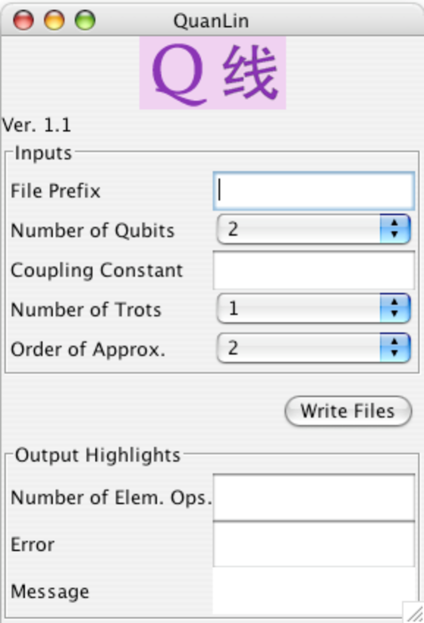
Figure 7: Control Panel of QuanLin

The Control Panel for QuanLin is almost identical to that for QuanTree. The significance of the various data fields in the Control Panel for QuanLin is the same as for QuanTree.

3.3 Output Files

Figs.8, 9, 10, were all generated in a single run of QuanLin (by pressing the Write Files button just once). They are examples of what we call the Log File, English File, and Picture File, respectively, of QuanLin. These files are analogous to their namesakes for QuanTree. They follow the same rules.

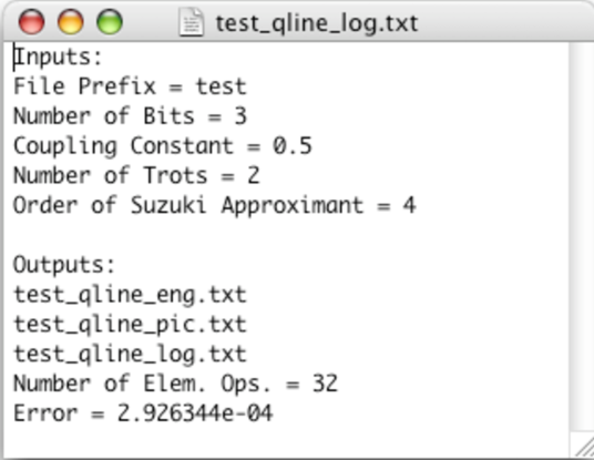
Figure 8: Log File generated by QuanLin

Figure 9: English File generated by QuanLin

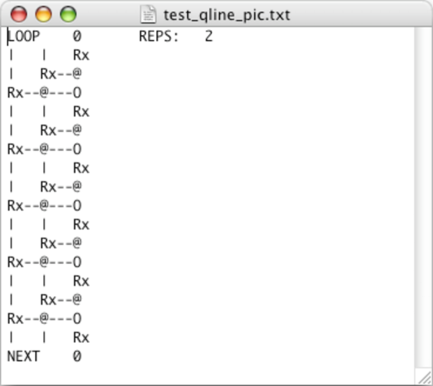
Figure 10: Picture File generated by QuanLin

References

- [1] R.R. Tucci, “A Rudimentary Quantum Compiler(2cnd Ed.)”, arXiv:quant-ph/9902062 . Qubiter software available at www.ar-tiste.com/qubiter.html
- [2] QuanTree and QuanLin software available at www.ar-tiste.com/QuanSuite.html
- [3] E. Farhi, J. Goldstone, S. Gutmann, “A Quantum Algorithm for the Hamiltonian NAND Tree”, arXiv:quant-ph/0702144
- [4] R.R.Tucci, “How to Compile Some NAND Formula Evaluators”, arXiv:0706.0479
- [5] G.H. Golub and C.F. Van Loan, Matrix Computations, Third Edition (John Hopkins Univ. Press, 1996).