Nonlinear behavior of bosons in anisotropic optical lattices

Abstract

We investigate the behavior of an array of Bose-Einstein condensate tubes described by means of a Bose-Hubbard Hamiltonian. Using an anisotropic non-polynomial Schrödinger equation we link the macroscopic parameters in the Bose-Hubbard Hamiltonian to the ones that are tunable in experiments. Using a mean field approach we predict that increasing the optical lattice strength along the direction of the tubes, the condensate can experience a reentrant transition between a Mott insulating phase and the superfluid one.

1 Introduction

Since Greiner et al. first succeeded at storing a Bose-Einstein condensate in a two-dimensional array of narrow tubes using an optical lattice [1], experimental progress on low-dimensional Bose systems has been tremendous. To name but a few highlights, the Mott transition was observed in three [2], one [3], and two dimensions [4, 5], and in 1D a Tonks-Girardeau gas has been realized [6, 7]. Moreover, in 2D the Kosterlitz-Thouless transition was observed [9, 8]. The dimensional crossover between three, two, and one dimensions for bosons in an optical lattice was studied theoretically using Tomonaga-Luttinger liquid (TLL) theory in Refs. [11, 10] and using Monte Carlo simulations in Ref. [12]. These references studied 2D or 3D optical lattices in which atoms can tunnel easily along one Cartesian direction but not along the others. The system can then be described as an array of tubes of bosons, which may or may not be mutually phase coherent. As the tunneling between tubes is varied, such a system will undergo a transition from a 3D superfluid (3D SF) to a 2D Mott insulating phase (2D MI), which consists of a decoupled array of 1D tubes. Similarly, if the tunneling probability along all three Cartesian directions are made unequal, a 2D SF state can be realized, in which there is superfluidity within separate 2D layers but no coherence between them. These transitions are present only if the tubes have finite length.

The theoretical approaches used in Refs. [11, 10, 12] are able to describe phase fluctuations within the tube-like filaments of bosons, but they do not capture any nonlinear effects due to the possible variation in the width of these tubes. Gross-Pitaevskii theory describes such variations [13]; however, it does so at the expense of not being able to account for phase fluctuations. Keeping these limitations in mind, we offer in this Letter a description that is complementary to those of Refs. [11, 10, 12], using Gross-Pitaevskii theory in order to understand how nonlinear effects may affect the phase transitions in this peculiar type of optical lattice. Such effects become important if the potential barriers along the strongly coupled direction are so weak that each tube can be considered as a quasi-1D Bose-Einstein condensate and the number of bosons is large. It will be shown that such nonlinear effects can give rise to a reentrant Mott transition in the array of 1D tubes.

The dilute Bose gas in an external potential $V_{ext}(\mathbf{r})$ is described by the second quantized Hamiltonian

$$\hat{H}[\hat{\psi},\hat{\psi}^{\dagger}]=\int d\mathbf{r}\Bigg{[}\frac{\hbar^{2}}{2m}|\nabla\hat{\psi}(\mathbf{r})|^{2} + V_{\mathrm{ext}}(\mathbf{r})\,|\hat{\psi}(\mathbf{r})|^{2}$$

$$+ \frac{g}{2}\,|\hat{\psi}(\mathbf{r})|^{4}\Bigg{]}\,.$$

The physical setting consists of a two-dimensional optical lattice in the $x$ and $y$ plane with period $d_{x}$ and $d_{y}$, creating a square array of tubes which develop along the $z$ direction. Moreover a weaker optical potential parallel to the tubes is added, so that in the present case the external potential is given by

$$V_{\mathrm{ext}}(x,y,z) = -\frac{V_{x}}{2}\,\cos\frac{2\pi\,x}{d_{x}}-\frac{V_{y}}{2}\,\cos\frac{2\pi\,y}{d_{y}}$$

$$+ \frac{V_{z}}{2}\,\cos\frac{2\pi\,z}{d_{z}}\,.$$

As in Ref. [14] the many-body wavefunction of the gas $\hat{\psi}(\mathbf{r})$ is rewritten as a sum of local operators

$$\hat{\psi}(\mathbf{r})=\sum_{j_{x}j_{y}k}\phi_{\revision{j_{x}j_{y}}k}(\mathbf{r})\,\hat{b}_{jk}\,,$$ (3)

where $\phi_{j_{x}j_{y}k}(\mathbf{r})=\phi_{k}(x+j_{x}\,d_{x},y+j_{y}\,d_{y},z)$ and each $\hat{b}_{jk}$ acts on the $k^{th}$ state of the $j^{th}$ tube. The $\phi_{k}$ are a complete set of wavefunctions. In the present setting we expect only the lowest energy state to be occupied, so that it is possible to drop the $k$ index from (3). Using expression (3) the second quantized grand potential

$$\hat{G}[\hat{\psi},\hat{\psi}^{\dagger}]=\hat{H}[\hat{\psi},\hat{\psi}^{\dagger}]-\mu_{\mathrm{G}}\hat{N}[\hat{\psi},\hat{\psi}^{\dagger}]$$ (4)

can be rewritten

$$\hat{G}= - \sum_{j}\Big{[}t_{x}\,\hat{b}^{\dagger}_{j_{x}}\hat{b}_{j_{x}+1}+t_{y}\,\hat{b}^{\dagger}_{j_{y}}\hat{b}_{j_{y}+1}+\mathrm{h.c.}\Big{]}$$

$$+ \frac{U}{2}\sum_{j}\hat{n}_{j}(\hat{n}_{j}-1)-\mu\sum_{j}\hat{n}_{j}\,,$$

where $j=(j_{x},j_{y})$, $\hat{n}_{j}=\hat{b}_{j}^{\dagger}\hat{b}_{j}$, and the inter-tube tunneling matrix elements are

$$t_{\alpha}= - \int d\mathbf{r}\,\Big{[}(\mathbf{\nabla}\phi_{j_{\alpha}})^{*}\cdot\mathbf{\nabla}\phi_{j_{\alpha}+1}$$

$$+ V_{\mathrm{ext}}(x,y,z)\,\phi_{j_{\alpha}}^{*}\,\phi_{j_{\alpha}+1}\Big{]}\,,$$

with $\alpha=\{x,y\}$. The in-tube interaction energy is

$$U=g\,\int d\mathbf{r}\,|\phi(\mathbf{r})|^{4}\,,$$ (7)

$$\mu=-\int d\mathbf{r}\,\left[\frac{\hbar^{2}}{2m}|\mathbf{\nabla}\phi(\mathbf{r})|^{2}+|\phi(\mathbf{r})|^{2}\,V_{\mathrm{ext}}(\mathbf{r})\right]+\mu_{\mathrm{G}}\,,$$ (8)

where $\mu_{\mathrm{G}}$ is a constant that fixes the number $N_{\mathrm{tot}}$ of particles in the whole system and $g=4\pi\hbar^{2}a_{s}/m$.

We assume that the external potential (1) along the $x$ and $y$ direction is very strong, so that the behavior of each tube can be described by a one-dimensional approximation of the Gross-Pitaevskii equation (cf. [13]). This approach is not appropriate to study the behavior of separate sites, since the number of particles would be too small to get accurate results; it is however expected to work in this context since each tube spans over many lattice sites. The non-polynomial Schrödinger equation (NPSE)  [16] has proven itself to be an excellent means to describe such many particle-systems. The main difference of this approach compared with the TLL description [11] is that it is possible to consider explicitly the transverse width of each tube, therefore studying the nonlinear effects due to the finite density on the behavior of the system. The main assumption of this work consists in taking the groundstate of the NPSE as the Wannier function $\phi(x,y,z)$ that appears in the expression of $t$, $U$, and $\mu$. In this way it is possible to link the physical parameters that are tunable in a real experiment to the macroscopic ones in the Bose-Hubbard Hamiltonian. Notice that in general $V_{x}\neq V_{y}$, so an anisotropic version of the NPSE is needed.

2 Anisotropic NPSE

We suppose that the confining potential in the transverse direction is strong enough so that the behavior of each tube is well described considering a harmonic external potential

$$V_{\mathrm{tube}}(\mathbf{r}) \approx \left[\frac{m\,\omega_{x}^{2}}{2}\,x^{2}+\frac{m\,\omega_{y}^{2}}{2}\,y^{2}\right]+\frac{V_{z}}{2}\,\cos\Big{(}\frac{2\pi}{d_{z}}\,z\Big{)}$$ (9)

$$= \frac{m\,\omega_{y}^{2}}{2}\left[\Lambda\,x^{2}+y^{2}\right]+\frac{V_{z}}{2}\,\cos\Big{(}\frac{2\pi}{d_{z}}\,z\Big{)}\,,$$

where

$$\omega_{y}=\frac{\sqrt{2}\pi}{d_{y}}\,\sqrt{\frac{V_{y}}{m}}\,,$$ (10)

and

$$\Lambda=\frac{\omega_{x}^{2}}{\omega_{y}^{2}}=\frac{V_{x}}{V_{y}}\,.$$ (11)

Therefore the wavefunction of each tube is factorized as

$$\phi(\mathbf{r})=\frac{\Lambda^{\frac{1}{8}}}{\sqrt{\pi}\,\eta(z)}\exp\Big{[}-\frac{1}{2\,\eta(z)}\big{(}\sqrt{\Lambda}\,x^{2}+y^{2}\big{)}\Big{]}\\ \times f(z)\,,$$ (12)

where

$$\Lambda=\frac{V_{x}}{V_{y}}\,.$$ (13)

We note that the approximation of the Wannier functions by Gaussians is known to introduce quite large quantitative errors when computing the tunneling matrix elements [13]. Nevertheless, since the Gross-Pitaevskii equation does not allow an easy treatment using Bloch theory, it is very hard to improve on the Gaussian approximation.

Following the steps in Ref. [16] an equation for the longitudinal part of each tube is derived. The energy functional for the Bose-Einstein condensate in each tube is

$$H[\phi,\phi^{*}]=\int d\mathbf{r} \Big{[} \frac{\hbar}{2m}|\nabla\phi(\mathbf{r})|^{2}$$

$$+ V_{\mathrm{tube}}(\mathbf{r})\,|\phi(\mathbf{r})|^{2}$$

$$+ \frac{g}{2}\,|\phi(\mathbf{r})|^{4}\Big{]}\,.$$

Substituting (12) into (2) it is possible to carry out the integration along $x$ and $y$. Dropping the terms proportional to $\eta^{\prime}(z)$ [15] and minimizing with respect to $\eta$ and $f^{*}$ the following equations are obtained:

$$\Big{[} - \frac{\hbar}{2\,m}\frac{d^{2}}{dz^{2}}+\frac{V_{z}}{2}\,\cos\frac{2\pi}{d_{z}}z$$

$$+ \,\revision{\frac{1+\sqrt{\Lambda}}{2}\,\hbar\,\omega_{y}}\,\frac{1+\frac{3}{2}\gamma\,|f(z)|^{2}}{\sqrt{1+\gamma\,|f(z)|^{2}}}\Big{]}\,f(z)$$

$$= \mu\,f(z)\,,$$

$$\eta_{y}(z)=a_{y}\,\left(1+\gamma\,|f(z)|^{2}\right)^{\frac{1}{4}}\,,$$ (16)

where $a_{y}=\sqrt{\hbar/(m\omega_{y})}$ and

$$\gamma=4N\,a_{s}\,\frac{\Lambda^{\frac{1}{4}}}{1+\sqrt{\Lambda}}\,.$$ (17)

Notice that Ref. (2) reduces to the previously obtained NPSE [16] in the case $\Lambda=1$.

3 Bose-Hubbard Parameters

Using (12) as an ansatz for the condensate wavefunction it is possible to express $t_{x}$, $t_{y}$, $\mu$, and $U$ in terms of integrals of $f(z)$ and $\eta(z)$. The expression for $t_{y}$ is

$$t_{y}=-\int dz\,\left[\frac{\hbar^{2}}{2m}\,A(z)+\frac{\hbar^{2}}{2m}\,B(z)+C(z)\right]\,,$$ (18)

where

$$A(z) = \int dx\,dy\Big{[}\Big{(}\frac{\partial\phi_{j_{y}}}{\partial x}\Big{)}^{*}\frac{\partial\phi_{j_{y}+1}}{\partial x}$$ (19)

$$~{}~{}~{}~{}~{}~{}~{}~{}~{}~{}~{}~{}~{}+\Big{(}\frac{\partial\phi_{j_{y}}}{\partial y}\Big{)}^{*}\frac{\partial\phi_{j_{y}+1}}{\partial y}\Big{]}$$

$$= \frac{\mathrm{exp}\left(-\frac{d_{y}^{2}}{4\,\eta_{y}(z)^{2}}\right)}{4\eta_{y}(z)^{2}}\,|f(z)|^{2}$$

$$~{}~{}\times\,\left(2\,(1+\sqrt{\Lambda})\,\eta_{y}(z)^{2}-d_{y}^{2}\right)\,,$$

$$B(z) = \int dx\,dy\left(\frac{\partial\phi_{j_{y}}}{\partial z}\right)^{*}\frac{\partial\phi_{j_{y}+1}}{\partial z}$$

$$= \mathrm{exp}\left(-\frac{d_{y}^{2}}{4\,\eta_{y}(z)^{2}}\right)\,|f^{\prime}(z)|^{2}\,,$$

and

$$C(z) = \int dx\,dy\,V_{\mathrm{ext}}(x,y,z)\,\phi_{j_{y}}^{*}\,\phi_{j_{y}+1}$$

$$= \frac{1}{2}\,\mathrm{exp}\left(-\frac{d_{y}^{2}}{4\,\eta_{y}(z)^{2}}\right)\Bigg{[}V_{z}\,\cos\left(\frac{2\pi\,z}{d_{z}}\right)$$

$$~{}~{}-V_{x}\,\mathrm{exp}\left(-\frac{\pi^{2}\eta_{y}(z)^{2}}{\sqrt{\Lambda}\,d_{x}^{2}}\right)$$

$$~{}~{}+V_{y}\,\mathrm{exp}\left(-\frac{\pi^{2}\eta_{y}(z)^{2}}{d_{y}^{2}}\right)\Bigg{]}\,|f(z)|^{2}\,.$$

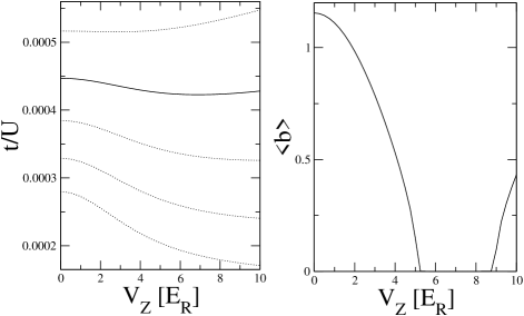
Figure 1: Left panel: behavior of $t/U$ as a function of $V_{z}$ for $n_{\mathrm{cell}}=1,2,3,4,5$, while $V_{x}=V_{y}=26.4E_{\mathrm{R}}$; for a system of length $L$ the parameter is scaled according to (24). Right panel: MF order parameter $\langle b\rangle$ against $V_{z}$ for the case $n_{\mathrm{cell}}=4$ and $L=6$ ($2.55\mathrm{\mu m}$).

Consistently with the NPSE approximation the terms proportional to $\eta^{\prime}(z)$ and $\eta^{\prime}(z)^{2}$ have been omitted. The expression for $t_{x}$ is obtained from $t_{y}$ switching the indices $x$ and $y$, and changing $\Lambda$ to $\Lambda^{-1}$. The integral for $U$ gives

$$U = g\int dx\,dy\,dz\,|\phi|^{4}$$

$$= g\,\bigg{(}\frac{V_{x}}{V_{y}}\bigg{)}^{\frac{1}{4}}\,\int dz\left[\frac{|f(z)|^{4}}{2\pi\,\eta_{y}(z)^{2}}\right]\,.$$

Switching the indices $x$ and $y$ leaves the value of $U$ invariant, so that the expression for the self-interaction energy of each tube is consistent with the symmetry of the problem.

In order to make explicit calculations we consider a system of ⁸⁷Rb atoms, whose atomic interaction is repulsive ($a_{s}=5.77\,\mathrm{nm}$). The lattice is a simple cubic one, with $d_{z}=d_{y}=d_{z}=425\mathrm{nm}$. Equation (2) is solved for $f(z)$ and $\eta(z)$ with periodic boundary conditions over a single cell by means of a self-consistent approach. The length of the tube affects the numerical results through the normalization of the function $f(z)$, so that using periodic boundary conditions over $L$ cells the value of $t_{\alpha}$ ($\alpha=\{x,y\}$) is left invariant and $U$ scales down as $1/L$, i.e. $t_{L}=t$ while

$$U_{L}=\frac{U}{L}\,,$$ (23)

where $t_{L}$ and $U_{L}$ denote the values of $t$ and $U$ for a system of tubes with length $L$. Notice that

$$\left(\frac{t_{\alpha}}{U}\right)_{L}=L\,\frac{t_{\alpha}}{U}\,.$$ (24)

Denoting by $n_{\mathrm{cell}}$ the number of particles in each longitudinal well, then the number of particles $n_{\mathrm{tube}}$ in each tube is

$$n_{\mathrm{tube}}=L\,n_{\mathrm{cell}}\,.$$ (25)

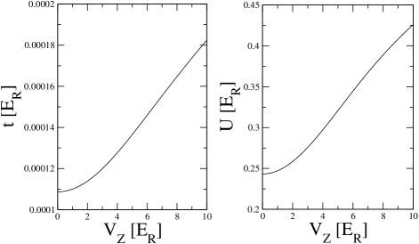
Figure 2: Behavior of $t$ (left panel) and $U$ (right panel) as a function of $V_{z}$ for $n_{\mathrm{cell}}=4$, while $V_{x}=V_{y}=26.4E_{\mathrm{R}}$.

At first we focus on an isotropic case, i.e. a situation in which $V_{x}=V_{y}=26.4\,E_{\mathrm{R}}$, where $E_{\mathrm{R}}$ is the recoil energy for a wavelength of 780 nm. Defining $t=t_{x}=t_{y}$, in Fig. 1 (left panel) there appears the behavior of $t/U$ while varying $V_{z}$ from $0$ to $10\,E_{\mathrm{R}}$, for $n_{\mathrm{cell}}=1,2,3,4,5$. According to Fig. 1, for $n_{\mathrm{cell}}=4$ the ratio $t/U$ decreases until $V_{z}\approx 7\,E_{\mathrm{R}}$, then it begins to rise. It is known [17, 18] that the Mott insulating phase appears as a set of “lobes” in the plane $\mu/U$-$t/U$, each one corresponding to a precise number of particles $n_{\mathrm{tube}}$ for each tube; outside of the 2D MI zone the system moves along lines of constant $n_{\mathrm{tube}}$. The initial decrease and subsequent decrease of $t/U$ therefore means that for an appropriate length of the tubes the system can cross the 3D SF - 2D MI transition twice. In order to give an estimate of the critical potential strength a mean field (MF) approach is employed (see for example [19, 18]). The MF order parameter is given by the expectation value of the destruction operator $\langle b\rangle$. Figure 1 (right panel) plots the behavior of this parameter for $n_{\mathrm{cell}}=4$ and $L=6$ ($2.55\mathrm{\mu m}$). The bounded interval in which the superfluid phase vanishes is a clear consequence of the nonlinear behavior of the system.

In order to understand the physical meaning of this phenomenon, the plot in Fig. 2 shows the behavior of $t$ and $U$ against $V_{z}$ separately for the case $n_{\mathrm{cell}}=4$. Increasing the longitudinal optical lattice $f(z)$ becomes narrower, thus raising the value of $U$ (3), while at the same time the wavefunction widens in the radial direction, increasing the tunneling rate $t$ (19). At first $U$ rises faster than $t$ but for $t\approx 7\,E_{\mathrm{R}}$ this relation is reversed. The observed nonlinear effect is therefore the result of a competition between $t$ and $U$.

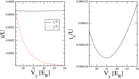
Figure 3: Left panel: plot of $t_{x}/U$ and $t_{y}/U$ as a function of $V_{y}$, while $V_{x}=26.4\,E_{\mathrm{R}}$, $V_{z}=5\,E_{\mathrm{R}}$, and $n_{\mathrm{cell}}=4$. Right panel: the behavior of $t_{x}/U$ is plotted in more detail for the same physical parameters.

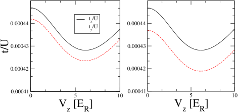
Figure 4: Behavior of $t_{x}/U$ and $t_{y}/U$ as a function of $V_{z}$ while $V_{x}=26.4\,E_{\mathrm{R}}$ and $n_{\mathrm{cell}}=4$; left panel: $V_{y}=26.45\,E_{\mathrm{R}}$, right panel: $V_{y}=26.5\,E_{\mathrm{R}}$.

So far it has been considered the isotropic case, in which $t_{x}$ is identical to $t_{y}$. That is no longer true in an anisotropic setting, i.e., one in which $V_{x}\neq V_{y}$. Figure 3 (left panel) shows the behavior of $t_{x}$ and $t_{y}$ upon varying $V_{y}$, with an occupation number $n_{\mathrm{cell}}=4$, keeping $V_{x}$ and $V_{z}$ fixed at $26.4\,E_{\mathrm{R}}$ and $5\,E_{\mathrm{R}}$ respectively. It is shown that while $t_{x}$ varies very little for different values of $V_{y}$, $t_{y}$ decreases exponentially. In the right panel of Fig. 3 is plotted in detail $t_{x}$ against $V_{y}$ for the same physical parameters, showing that $t_{x}$ has a minimum for $V_{y}\approx 35\,E_{\mathrm{R}}$. These results suggest that upon increasing $V_{y}$ the boson gas enters a 2D SF phase, in which the system is organized in superfluid layers along the $y$ direction. Moreover the behavior of $t_{x}$ suggests that - if all the parameters are carefully tuned - these layers could experience a reentrant transition between the 2D SF phase and the 2D MI one, in which each tube is isolated from the others.

The asymmetric case provides another interesting phenomenon. Figure 4 shows the situation in which $V_{x}=26.4\,E_{\mathrm{R}}$, and $n_{\mathrm{cell}}=4$, for $V_{y}=26.45\,E_{\mathrm{R}}$ (left panel) and $V_{y}=26.5\,E_{\mathrm{R}}$ (right panel). Increasing $V_{y}$, the curves of $t_{x}$ and $t_{y}$ become more and more separated; in particular the curve for $t_{y}$ shifts downwards, and its minimum moves to the left. This behavior suggests a curious effect in which - upon increasing $V_{z}$ - the system may move from a 3D SF phase to a 2D SF one, from this to a 2D MI phase and then back again to the 2D SF.

4 Conclusions

In this Letter we have studied the behavior of a 2D array of strongly elongated tubes of bosons in an optical lattice, employing the Bose-Hubbard Hamiltonian in order to describe the 3D SF - 2D MI transition. Using the NPSE (2) to compute the groundstate in each tube it was possible to link the parameter $t$ and $U$ of the Bose-Hubbard Hamiltonian to the physical parameters of the atom gas. Using this approach an observable nonlinear effect is found: we predict that in an array of ⁸⁷Rb tubes $2.55\,\mathrm{\mu m}$ long, with $d_{x}=d_{y}=d_{z}=425\,\mathrm{nm}$, $V_{x}=V_{y}=26.4\,E_{\mathrm{R}}$, and an occupation number of 4 atoms for each cell, the system goes through the 3D SF - 2D MI transition twice while increasing $V_{z}$. The system itself is found to be in the insulating phase for $V_{z}$ between $\sim 5\,E_{R}$ and $\sim 8\,E_{R}$. In addition, in the anisotropic case, our results suggest that the nonlinear behavior of the system should cause a reentrant transition between the 2D SF phase, in which the gas is organized in superfluid layers, and the 2D MI phase, where each tube acts independently. A real experiment will be complicated by the fact that not all the tubes would be equally long and the occupation number fluctuates. Moreover, due to the approximations we have made, the most severe being the assumption of a Gaussian profile for the basis functions and the neglect of quantum fluctuations in the phase, the exact numbers are expected to differ from our predictions. We argue that the qualitative analysis should hold, i.e., an experiment should in certain parameter regimes show a dip in the phase coherence while varying $V_{z}$, since this feature depends crucially only on the fact that the tunneling $t$ and on-site interaction energy $U$ exhibit different functional dependencies on the width of the tube-like condensates.

5 10

Georges A. arXiv:cond-mat/07021222007

- [1] \NameGreiner M., Bloch I., Mandel O., Hänsch T. W., and Esslinger T. \REVIEWPhys. Rev. Lett.872001160405
- [2] \NameGreiner M., Mandel O., Esslinger T., Hänsch T. W., and Bloch I. \REVIEWNature415200239
- [3] \NameStöferle T., Moritz H., Schori C., Köhl M., and Esslinger T. \REVIEWPhys. Rev. Lett.922004130403
- [4] \NameKöhl M., Moritz H., Stöferle T., Schori C., and Esslinger T. \REVIEWJournal of Low Temperature Physics1382005635
- [5] \NameSpielman I. B., Phillips W. D., and Porto J. V. \REVIEWPhys. Rev. Lett.982007080404
- [6] \NameParedes B., Widera A., Murg V., Mandel O., Fölling S., Cirac I., Shlyapnikov G. V., Hänsch T. W., and Bloch I. \REVIEWNature (London)4292004277
- [7] \NameKinoshita T., Wenger T., and Weiss D. S. \REVIEWScience30520041125
- [8] \NameSchweikhard V., Tung S., and Cornell E. A. \REVIEWPhys. Rev. Lett.992007030401
- [9] \NameHadzibabic Z., Krüger P., Cheneau M., Battelier B., and Dalibard J.B. \REVIEWNature44120061118
- [10] \NameGangardt D. M., Pedri P., Santos L., and Shlyapnikov G. V. \REVIEWPhys. Rev. Lett.962006040403
- [11] \NameHo A. F., Cazalilla M. A., and Giamarchi T. \REVIEWPhys. Rev. Lett.922004130405
- [12] \NameBergkvist S., Rosengren A., Saers R., Lundh E., Rehn M., and Kastberg A. \REVIEWPhys. Rev. Lett.992007110401
- [13] \Namevan Oosten D., van der Straten, and Stoof H.T.C. \REVIEWPhys. Rev. A672003033606
- [14] \NameJaksch D., Bruder C., Cirac J. I., Gardiner C. W., and Zoller P. \REVIEWPhys. Rev. Lett8119983108-3111
- [15] \NameSalasnich L., Parola A., and Reatto L. \REVIEWPhys Rev. A652002043614
- [16] \NameSalasnich L., Cetoli A., Malomed B.A. and Toigo F. \REVIEWPhys Rev. A752007033622
- [17] \NameFisher M. P. A., Weichman P. B., Grinstein G., and Fisher D. S. \REVIEWPhys. Rev. B40 (1)1989546-570
- [18] \NameSachdev S. \BookQuantum Phase Transitions \PublCambridge University Press \Year1999