Chaos in an intermittently driven damped oscillator

Abstract

We observe chaotic dynamics in a damped linear oscillator, which is driven only at certain regions of phase space. Both deterministic and random drives are studied. The dynamics is characterized using standard techniques of nonlinear dynamics. Interchanging roles of determinism and stochasticity is also considered.

1 Introduction

It is generally known that continuous linear systems cannot exhibit chaotic time evolution. However recently it has been shown that chaotic behavior can occur in systems without explicit non linearities. Hirata et.al. [1] have shown that continuous chaotic wave forms can be constructed by the superposition of certain pulse basis functions. In a linear second order filter driven by randomly polarized pulses, chaotic behavior is observed when the time series is viewed backwards in time [2]. Further they have shown that by reversing the time series, folded band chaos similar to Rössler attractor can also be synthesized [3]. Even if the time reversal is not physical, this reveals the importance of pure randomness which is associated with chaotic behavior. Studies in this direction are important in understanding the relation between randomness, determinism and complexity in dynamical systems.

We study a weakly damped driven linear oscillator where the oscillator and the drive are coupled only when the trajectory is in a thin strip in the phase space. This modification introduces strong nonlinearities required for chaotic behavior. First we consider the oscillator coupled to a deterministic drive. Then we consider a random forcing. We show that the attractors formed by both the deterministic and random forcing are similar in many respects.

2 Basic model

The driven damped linear oscillator is well known and is important in almost all branches of physical science. The dynamics of this system satisfies the equation,

$$\frac{d^{2}x}{dt^{2}}+\gamma\frac{dx}{dt}+\Omega^{2}x = a\sin(\omega t).$$ (1)

The parameters in the equation are $\gamma$, the damping coefficient, $\Omega$, the angular frequency of the oscillator and $\omega$ the frequency of the drive. Such a system shows periodic behavior after the initial transients have vanished.

Our basic model is the one in which the system is driven only in a thin strip of the phase space. We choose the origin as the location of the strip because orbits with lower energy may not encounter the strip, if it is located far from the origin. Such orbits will spiral towards zero as in the case of an ordinary damped oscillator. When not driven, the oscillator performs a damped motion and the drive runs freely. First we consider a deterministic drive. The dynamics is characterized using standard techniques. Also the behavior under parameter variations is studied. Later we discuss the effect of replacing the deterministic driving term with a stochastic one.

3 Deterministic driving

3.1 Dynamical equations

The equation 1 modified accordingly by the addition of a new term $\mu(s,x)$ as,

$$\frac{d^{2}x}{dt^{2}}+\gamma\frac{dx}{dt}+\Omega^{2}x = \mu(s,x)a\sin(\omega t)$$ (2)

where,

$$\mu(s,x)=\left\{\begin{array}[]{ll}1&$if$~{}\mid x\mid~{}\leq s\\ 0&$otherwise$.\\ \end{array}\right.$$ (3)

Thus with a deterministic drive, what the dynamical equations represent is legitimate deterministic system in every sense.

3.2 Numerical results

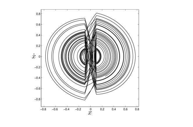
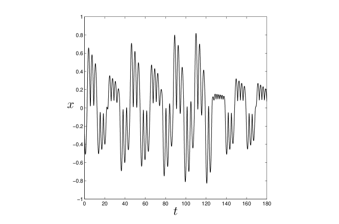
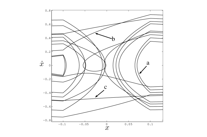
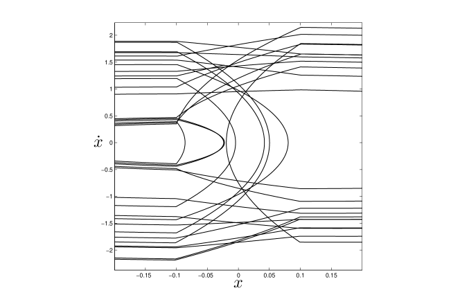
Numerical simulations were done using the Runge-Kutta algorithm with a step size of $10^{-3}$. We choose the following values for the parameters: $\Omega~{}=~{}1.0$, $\gamma~{}=~{}0.1$, $\omega~{}=~{}0.3$, $s=0.1$ and $a~{}=~{}2.5$. The parameters were chosen by numerical trials to express the concepts clearly, and are fixed during the evolution of the system in time. Fig.1 shows the phase space plot of the system. Note that there is a discontinuity in a strip of width $2s$ near $0$ in the the phase space, where the oscillator is coupled to the drive. A closer view of the strip is given in Fig. 4. It can be seen that the trajectories that approach the origin may either cross the strip with or without considerable modifications, or it may get reversed. Fig. 2 shows the time series $x(t)$ of the system. The amplitude of oscillations, and the number of

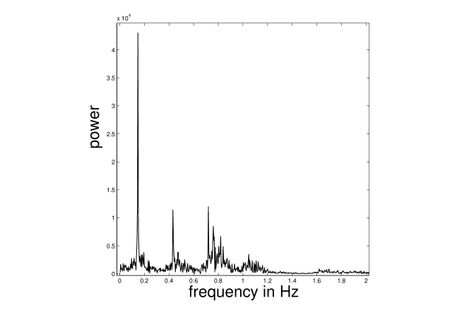
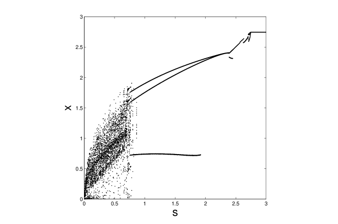
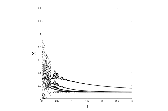
oscillations between two consecutive crossings of the strip are irregular. This corresponds to the phase space dynamics which consists of reflections in the strip and transitions which modify the trajectories. The power spectrum as shown in Fig. 3 is broad which confirms the aperiodic behavior in time. Varying the parameters $\gamma$ and $s$, the system exhibits both chaotic and periodic oscillations. From the bifurcation diagrams shown in Fig. 5 and Fig. 6, it can be seen that the chaotic behavior disappears for higher values of $\gamma$ and $s$. Also note that for $s~{}\simeq~{}1$ there is a transition to the case of an ordinary driven damped linear oscillator, where no chaotic behavior is expected.

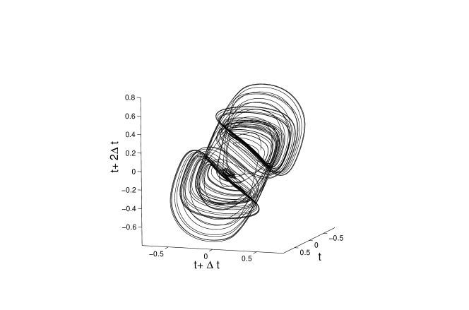
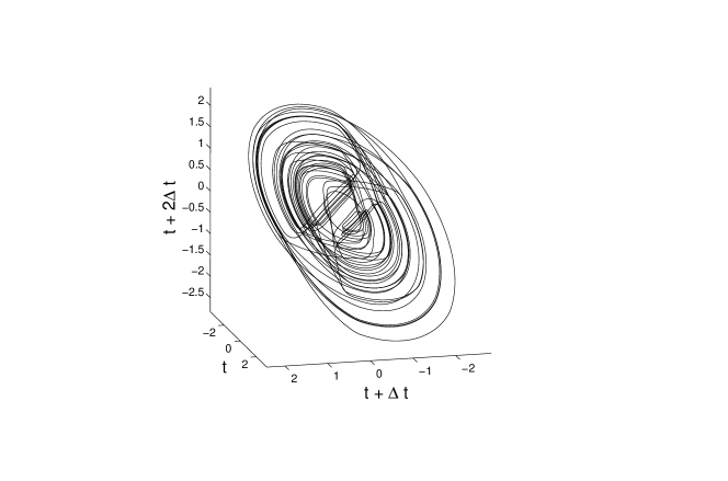
We used $DATAPLORE$ [4] for the analysis of the time series. The time delay required for reconstructing a timeseries is a widely discussed topic [5]. With a delay of 1.56, it is found that the autocorrelation function falls to $0.5$. With this delay, embedding dimension was calculated using False nearest neighbors method [6]. It is found that the percentage of nearest neighbors approaches zero with embedding dimension 3. Lyapunov Exponents were calculated with embedding dimension 3, number of nearest neighbors 37 and degree of the extrapolating polynomial 3. The obtained result is multiplied by the sampling frequency of the input signal to calculate the Lyapunov exponents. The Largest Lyapunov exponent is found to be $3.19$. We obtained 2.148 as the Kaplan-Yorke dimension. The reconstructed phase space of the attractor is shown in fig. 7 and is similar in appearance to other chaotic systems.

4 Random driving

4.1 Dynamical equations

Random forcing is achieved by the drive assuming a random value $\xi$ each time the phase space trajectory enters the strip. The amplitude of forcing $\xi$ is Gaussian random variable with variance $\sigma^{2}=\frac{1}{\sqrt{2}}$ and zero mean. We define $\chi(s,x)$ as follows,

$$\chi(s,x)=\left\{\begin{array}[]{ll}\xi&$if$~{}\mid x\mid~{}\leq s\\ 0&$otherwise$.\\ \end{array}\right.$$ (4)

Retaining $\mu(s,x)$ defined as in eq. 2 for comparison, the dynamical equation is,

$$\frac{d^{2}x}{dt^{2}}+\gamma\frac{dx}{dt}+\Omega^{2}x = a\mu(s,x)\chi(s,x)$$ (5)

4.2 Numerical results

When the oscillator is driven randomly, it is found that the attractor is still chaotic with the largest Lyapunov exponent equal to $2.92$ and a Kaplan-Yorke dimension of $2.31$ when embedded in three dimensions. The dynamics in phase space is similar to the one obtained with a deterministic drive as shown in Fig. 8. The reconstructed attractor (with time delay $\Delta t~{}=~{}1.1$) given in Fig. 9 is similar to the one obtained with a deterministic evolution.

5 Discussion

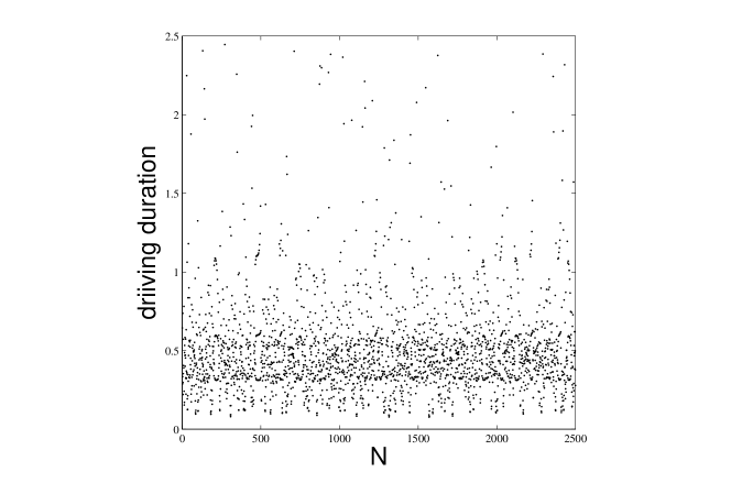
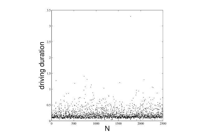
The effect of a forcing on the dynamics can depend on many factors. The most important are the amplitude and the time for which such a forcing persists. With Eq. 2 the dynamics of the system in terms of phase space variables is well defined. The only degree of freedom available for an irregular behavior is through the time interval in which the system is driven and is not driven. At the onset of chaos, it can be seen from Fig. 10 that the durations for which the driving persists are highly irregular. Also irregular are the intervals in which the system is not driven. This intermittent nature of the drive and irregular durations of the driving events are the only source of irregularities for a dynamics which is linear in every region of phase space. From Fig. 11, it can be seen that the random forcing applied to the oscillator also persists for irregular durations. Stochasticity as such is a source for irregularities in a system. But it may not be the same as the topological structure of an attractor demands. There, the intermittent driving and irregular driving durations play a significant role. It modifies the irregularities associated with the driving suitable for chaotic dynamics in the system. The durations for which the system is not driven are also irregular in a similar manner. Thus intermittency is significant to the chaotic behavior due to its role in synthesizing or seasoning the complexities that occur in the dynamics.

The damped oscillator, together with its drive, have got another very fundamental similarity with deterministic chaos. The phase space of a chaotic system is dense in periodic orbits, or, it contains infinitely many periodic orbits. None of these periodic orbits are stable, but they significantly influence the evolution of a system in the phase space. This aspect is important in considering the anatomy of the chaotic behavior exhibited by the system under consideration. Different periodicities arise due to different numbers of reflections and transmissions in the strip. The drive acts as the triggering mechanism for reflections or transmissions in the strip which facilitates smooth transitions between orbits of various periodicities. This is also the reason why the attractor structure remains similar under both deterministic and periodic drivings. Though physically similar, two driving schemes are completely different in a mathematical sense. Thus intermittently driven oscillator is an example where determinism can mimic stochasticity.

6 Conclusion

A Damped linear driven oscillator can exhibit chaotic behavior if the coupling between the drive and the oscillator are applied only at a narrow region of the phase space. Similar chaotic behavior can be observed with a purely random forcing. Though physically similar mechanisms exist for such a behavior, mathematically, they are different. We hope that this work has revealed yet another relation between randomness and determinism in nature.

7 Acknowledgments

One of the author(MPJ) acknowledges the council of scientific and industrial research (CSIR), New Delhi for financial support through a senior research fellowship (SRF). We also thank M. Lakshmanan and S. Rajesh for fruitful discussions.

Figure 1: Phase space trajectory of the oscillator ($\Omega~{}=~{}1.0$, $\gamma~{}=~{}0.1$, $\omega~{}=~{}0.3$, $s=0.1$ and $a~{}=~{}2.5$).

Figure 2: Time series of the system ($\Omega~{}=~{}1.0$, $\gamma~{}=~{}0.1$, $\omega~{}=~{}0.3$, $s=0.1$ and $a~{}=~{}2.5$).

Figure 3: Power spectrum of the time series $x(t)$ ($\Omega~{}=~{}1.0$, $\gamma~{}=~{}0.1$, $\omega~{}=~{}0.3$, $s=0.1$ and $a~{}=~{}2.5$).

Figure 4: Close view of the strip. Note the trajectories: a) reverse direction b) cross the strip but suffers deformation, c) cross the strip without considerable modification.

Figure 5: Bifurcation diagram obtained by varying the strip width $s$. Chaotic behavior disappears as the width of the strip is ($\Omega~{}=~{}1.0$, $\gamma~{}=~{}0.1$, $\omega~{}=~{}0.3$ and $a~{}=~{}2.5$).

Figure 6: Bifurcation diagram obtained by varying the damping coefficient $\gamma$. Chaotic behavior is suppressed as the damping is increased ($\Omega~{}=~{}1.0$, $\omega~{}=~{}0.3$, $s=0.1$ and $a~{}=~{}2.5$).

Figure 7: The delay reconstructed attractor ($\Omega~{}=~{}1.0$, $\gamma~{}=~{}0.1$, $\omega~{}=~{}0.3$, $s=0.1$, $a~{}=~{}2.5$ and $\Delta t~{}=~{}1.56$ ).

Figure 8: Close view of the phase space strip of a randomly driven oscillator.

Figure 9: The reconstructed attractor resulting from random driving ( $\Omega~{}=~{}1.0$, $\gamma~{}=~{}0.1$, $s=0.1$, $a~{}=~{}2.5$ and $\Delta t~{}=~{}1.1$).

Figure 10: Deterministic drive: the duration of the driving episodes. N represents $N^{th}$ driving event.

Figure 11: Random forcing: the duration of the driving episodes. N represents $N^{th}$ driving event ($\Delta t~{}=~{}0.25s$, $\Omega~{}=~{}1.0$, $\gamma~{}=~{}0.1$, $s=0.1$ and $a~{}=~{}2.5$).

References

- [1] Y. Hirata and K. Judd, ”Constructing dynamical systems with specified symbolic dynamics”, Chaos 15, 33102 (2005).
- [2] N. J. Corron, S. T. Hayes, S. D. Pethel and J. N. Blakely, ”Chaos without Nonlinear Dynamics”, Phys. Rev. Lett 97, 24101(2006).
- [3] N. J. Corron, S. T. Hayes, S. D. Pethel and J. N. Blakely, ”Synthesizing folded band chaos”, Phys. Rev. E 75, 45201(2006).
-
[4]
The official Weblink to Dataplore is
http://www.ixellence.com/en/analyse/dataplore_index.html and the
online manual can be found under
http://www.ixellence.com/onlinedocu/index_dp.html
- [5] P. S. Addison, Fractals and Chaos, (Overseas Press, New Delhi 2005).
- [6] H. Kantz and T. Schreiber, Nonlinear time series analysis, (Cambridge University Press, Cambridge 1997).