Unparticle Searches Through Gamma Gamma Scattering

Abstract

We investigate the effects of unparticles on $\gamma\gamma\to\gamma\gamma$ scattering for photon collider mode of the future multi-TeV $e^{+}e^{-}$ linear collider. We show the effects of unparticles on the differential, and total scattering cross sections for different polarization configurations. Considering 1-loop Standard Model background contributions from the charged fermions, and $W^{\pm}$ bosons to the cross section, we calculate the upper limits on the unparticle couplings $\lambda_{0}$ to the photons for various values of the scaling dimension $d(1<d<2)$ at $\sqrt{s}=0.5-5$ TeV.

I Introduction

Recently, a mind-blowing, and very interesting, new physics proposal has been presented by Georgi Georgi:2007ek . According to this proposal, there could be a scale invariant sector with a nontrivial infrared fixed point living at a very high energy scale. Since any theory with massive fields cannot be scale invariant, the Standard Model(SM) is not a scale invariant theory. Therefore, such a scale invariant sector, if any, should consist of massless fields and would interact with the SM fields at the very high energies. One of the most striking low energy properties of that proposal is that using the low energy effective theory considerations one can calculate the possible effects of such a scale invariant sector for the TeV scale colliders.

In the Ref.Georgi:2007ek , the fields of a very high energy theory with a nontrivial fixed point are called as BZ(for Banks-Zaks) fields according to Ref.Banks:1981nn . Interactions of BZ operators ${\cal O}_{BZ}$ with the SM operators ${\cal O}_{SM}$ are expressed by the exchange of particles with a very high energy mass scale ${\cal M}_{\cal U}^{k}$ in the following form

$$\frac{1}{{\cal M}_{\cal U}^{k}}{O}_{BZ}{O}_{SM}$$ (1)

where BZ, and SM operators are defined as ${O}_{BZ}\in{\cal O}_{BZ}$ with mass dimension $d_{BZ}$, and ${O}_{SM}\in{\cal O}_{SM}$ with mass dimension $d_{SM}$. Low energy effects of the scale invariant ${\cal O}_{BZ}$ fields imply a dimensional transmutation. Thus, after the dimensional transmutation Eq.(1) is given as

$$\frac{C_{\cal U}\Lambda_{\cal U}^{d_{BZ}-d}}{{\cal M}_{\cal U}^{k}}{O}_{\cal U}{O}_{SM}$$ (2)

where $d$ is the scaling mass dimension of the unparticle operator $O_{\cal U}$ (in Ref.Georgi:2007ek , $d=d_{\cal U}$ ), and the constant $C_{\cal U}$ is a coefficient function.

Using the low energy effective field theory approach, very briefly summarized above, in Refs Georgi:2007ek , and Georgi:2007si main properties of the unparticle physics are presented. A list of Feynman rules for the unparticles coupled to the SM fields, and several implications of the collider phenomenology are given in the Ref.Cheung:2007ue . In this paper, our calculations are based on the conventions of the Ref.Cheung:2007ue .

Searching for the new physics effects, the $e^{+}e^{-}$ linear colliders have an exceptional advantageous for its appealing clean background, and the possibility for the options of $e\gamma$, and $\gamma\gamma$ colliders based on it. Recently, for the new physics searches, as a multi-TeV energy electron-positron linear collider, the Compact Linear Collider(CLIC) proposed and developed at CERN, is seriously taken into account. Numerous works on the CLIC have been done so far clic . As other $e^{+}e^{-}$ linear colliders, the CLIC would have the options for $e^{-}e^{-},e\gamma$, and $\gamma\gamma$ collider options, and possibilities of polarized $e^{+},e^{-}$ beams. In this paper, we consider the $\gamma\gamma$ collider option of the CLIC, to search for the unparticle physics effects. Our results can easily be extended for other possible future multi TeV-scale linear electron-positron colliders. In Ref. Ginzburg:1983 , a detailed analysis on $\gamma\gamma$ option of an $e^{+}e^{-}$ collider has been given. Since $\gamma\gamma\to\gamma\gamma$ process can only occur at loop-level in SM it gives a good opportunity to test of new physics which has tree level contributions to the scattering amplitude. Regarding this process, as new physics searches, for example, supersymmetry gounaris1999 , large extra dimensions Cheung:1999ja ; davoudiasl1999 , and noncommutative space-time effects hewett2001 has been taken into account. Here, we study the effects of the unparticles on this process.

II Gamma Gamma Scattering

The lowest order SM contributions to the $\gamma\gamma\to\gamma\gamma$ process are 1-loop contributions of the charged fermions, and $W^{\pm}$ bosons. In the limits, for mandelstam parameters, $s,|t|,|u|>>M_{W}^{2}$, and using certain symmetry arguments given in the Ref.Jikia:1993tc ; gounaris1999 those 1-loop contributions can be expressed briefly. We present the corresponding 1-loop SM amplitudes in the Appendix A.1. Analysis of Fox et al. Fox:2007sy , highlights that the existence of the scalar unparticle operator leads to the conformal symmetry breaking when the Higgs operator gets the vacuum expectation value. If this symmetry breaking occurs at low energies some strong constraints are imposed on the unparticle sector. Here, we assume that the effects of unparticle sector on future high energy collider energies could be measurable.

Using the low energy effective field theory assumptions of Ref.s Georgi:2007si ; Cheung:2007ue , there are three tree level diagrams contributing to $\gamma(p_{1})\gamma(p_{2})\to\gamma(p_{3})\gamma(p_{4})$ scattering amplitude from the exchange of the scalar unparticle $U_{S}$ which can be expressed with the following amplitudes

$${M^{s}_{{\cal U}_{S}}}= \Big{[}\epsilon^{\mu}(p_{1})\big{[}4i\frac{\lambda_{0}}{\Lambda_{U}^{d}}[-p_{1}.p_{2}g_{\mu\nu}+p_{1\nu}p_{2\mu}]\big{]}\epsilon^{\nu}(p_{2})\Big{]}\Big{[}\epsilon^{\rho*}(p_{3})\big{[}4i\frac{\lambda_{0}}{\Lambda_{U}^{d}}[-p_{3}.p_{4}g_{\rho\sigma}+p_{3\sigma}p_{4\rho}]\big{]}\epsilon^{\sigma*}(p_{4})\Big{]}$$ (3)

$$\times\big{[}\frac{iA_{d}}{2\sin{d\pi}}[-(p_{1}+p_{2})^{2}]^{d-2}\big{]}$$

$${M^{t}_{{\cal U}_{S}}}= \Big{[}\epsilon^{\rho*}(p_{3})\big{[}4i\frac{\lambda_{0}}{\Lambda_{U}^{d}}[p_{1}.p_{3}g_{\mu\rho}-p_{1\rho}p_{3\mu}]\big{]}\epsilon^{\mu}(p_{1})\Big{]}\Big{[}\epsilon^{\sigma*}(p_{4})\big{[}4i\frac{\lambda_{0}}{\Lambda_{U}^{d}}[p_{2}.p_{4}g_{\nu\sigma}-p_{2\sigma}p_{4\nu}]\big{]}\epsilon^{\nu}(p_{2})\Big{]}$$ (4)

$$\times\big{[}\frac{iA_{d}}{2\sin{d\pi}}[-(p_{1}-p_{3})^{2}]^{d-2}\big{]}$$

$${M^{u}_{{\cal U}_{S}}}= \Big{[}\epsilon^{\sigma*}(p_{4})\big{[}4i\frac{\lambda_{0}}{\Lambda_{U}^{d}}[p_{1}.p_{4}g_{\mu\sigma}-p_{1\sigma}p_{4\mu}]\big{]}\epsilon^{\mu}(p_{1})\Big{]}\Big{[}\epsilon^{\rho*}(p_{3})\big{[}4i\frac{\lambda_{0}}{\Lambda_{U}^{d}}[p_{2}.p_{3}g_{\nu\rho}-p_{2\rho}p_{3\nu}]\big{]}\epsilon^{\nu}(p_{2})\Big{]}$$ (5)

$$\times\big{[}\frac{iA_{d}}{2\sin{d\pi}}[-(p_{1}-p_{4})^{2}]^{d-2}\big{]}$$

with

$$A_{d}=\frac{16\pi^{5/2}}{{(2\pi)}^{2d}}\frac{\Gamma(d+1/2)}{\Gamma(d-1)\Gamma(2d)}.$$ (6)

where $\lambda_{0}$ and $\Lambda_{U}$ are the effective coupling and the energy scale for scalar unparticle operator, respectively . We use the appropriate form of the scalar unparticle propagator, $\Delta_{F}(q^{2})=\frac{A_{d}}{2sin(d\pi)}(-q^{2})^{d-2}$. Since the mandelstam parameter $s>0$ there is a complex phase factor due to s-channel amplitude. Thus, for s-channel propagator one can consider $(-s^{2})^{d-2}=(s)^{d-2}e^{-id\pi}$ Cheung:2007ue . The implications of such a complex factor could be studied only through the interference terms . The interesting features of this phase through s-channel interferences between SM and unparticle amplitudes have been discussed by Georgi:2007si . In the calculations of the unpolarized and polarized cross sections, we use the expressions given in the Appendix. To give an idea about the unparticle effects on the unpolarized differential cross section $d\sigma/d\cos\theta$ with and without unparticle effects is plotted in Figure 1. In this figure, we choose $\lambda_{0}/\Lambda_{\cal U}=0.2$ TeV^-1, and the values $d=1.1$, $1.3$ and $d=1.5$ at $\sqrt{s_{ee}}=1$ TeV. One can see from Fig. 1, the unparticle effect increases while the scaling dimension $d$ approaches to 1. The unpolarized total cross section with respect to the center of mass energy of the mono-energetic photon beams with and without unparticle contributions is plotted in the Figure 2. For the unparticle effects in that plot, we assume, $\lambda_{0}/\Lambda_{\cal U}=0.1$ TeV^-1, and we compare the shape of the distribution for $d=1.1$, and $d=1.5$.

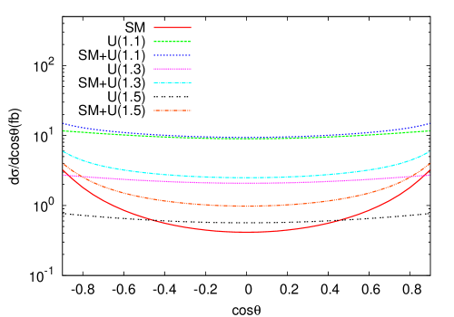
Figure 1: The unpolarized differential cross sections with pure SM, and SM+${\cal U}$ effects at $\sqrt{s_{ee}}=1$ TeV. For the unparticle effects, $\lambda_{0}/\Lambda_{\cal U}=0.2$ TeV^-1, $d=1.1$, $1.3$ and $d=1.5$.

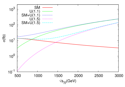
Figure 2: The unpolarized cross sections for SM, and SM+${\cal U}$. For the unparticle effects, $\lambda_{0}/\Lambda_{\cal U}=0.1$ TeV^-1, $d=1.1$, and $d=1.5$.

For the polarized cross section calculations of the back scattered photons, we define $M_{ijkl}$ to be a helicity amplitude of $\gamma\gamma\to\gamma\gamma$ scattering. And, we use the following definitions

$$|M(++)|^{2} = \sum_{i,j}|M(++ij)|^{2}$$ (7)

$$|M(+-)|^{2} = \sum_{i,j}|M(+-ij)|^{2}$$ (8)

where the summations are over the helicities of outgoing photons. Therefore, depending on the initial fermion polarization $P_{e}$, and the laser beam polarization $h_{l}$, the differential scattering cross section in terms of the average helicity $h_{\gamma}$ can be written as

$$\frac{d\sigma}{d\cos\theta} =\frac{1}{(64\pi)}\int_{x_{1min}}^{0.83}dx_{1}\int_{x_{2min}}^{0.83}dx_{2}\frac{f(x_{1})f(x_{2})}{\hat{s}}$$

$$\times \Big{[}\Big{(}\frac{1+h_{\gamma}(x_{1})h_{\gamma}(x_{2})}{2}\Big{)}\Big{|}M^{SM+{\cal U}_{S}}(++)\Big{|}^{2}+\Big{(}\frac{1-h_{\gamma}(x_{1})h_{\gamma}(x_{2})}{2}\Big{)}\Big{|}M^{SM+{\cal U}_{S}}(+-)\Big{|}^{2}\Big{]}$$ (9)

where $f(x)$ is the photon number density, and $h_{\gamma}$ is the average helicity function presented in the Appendix A.3, and as $\sqrt{s_{ee}}\equiv\sqrt{s}$ being the center of mass energy of the $e^{+}e^{-}$ collider, $\sqrt{\hat{s}}=\sqrt{x_{1}x_{2}s_{ee}}$ is the reduced center of mass energy of the back-scattered photon beams, and $x=E_{\gamma}/E_{e}$ is the energy fraction taken by the back-scattered photon beam. In our analysis, we follow the usual collider assumptions (for example Ref.sdavoudiasl1999 ; hewett2001 ) and we take $|h_{l}|=1$, and $|P_{e}|=0.9$. Also, since we consider the kinematical region $M_{W}^{2}/s,|M_{W}^{2}/t|,|M_{W}^{2}/u|<1$, in our analysis, we use the cuts $\pi/6<\theta<5\pi/6$, and $\sqrt{0.4}<x_{i}<x_{max}$ which have been used in the literature, where $x_{max}$ is the maximum energy fraction of the back-scattered photon, and its optimum value is 0.83.

In Figure 3, and Figure 4, to present schematic behavior of the polarized cross section with or without unparticle contributions, we plot the total cross section for two different polarization configurations of initial beams. We use the following definitions for the polarization configurations: $(++)\equiv(++++)=(P_{e1}=0.9,h_{l1}=1;P_{e2}=0.9,h_{l2}=1)$, and $(+-)\equiv(+-+-)=(P_{e1}=0.9,h_{l1}=-1;P_{e2}=0.9,h_{l2}=-1)$. Those figures could give an idea about the scaling dimension $d$ dependence of the unparticle contribution.

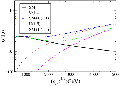
Figure 3: The total polarized cross sections for SM, and SM+${\cal U}$ with the polarization configuration $(++)$. Here, we assume $\lambda_{0}/\Lambda_{U}=0.1$ TeV^-1, $d=1.1$ and $1.5$.

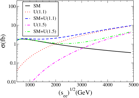
Figure 4: The total polarized cross sections for SM, and SM+${\cal U}$ with the polarization configuration $(+-)$. Here, we assume $\lambda_{0}/\Lambda_{U}=0.1$ TeV^-1, $d=1.1$ and $1.5$.

III Limits

Searching for the unparticle effects in a high energy $\gamma\gamma\to\gamma\gamma$ scattering, we extract the upper limits on the unparticle coupling $\lambda_{0}$ regarding the $95\%$ C.L. analysis. In the calculations, we use the standard chi-square analysis for the following $\chi^{2}$ function

$$\chi^{2}=\sum_{i}\left[{{{d\sigma_{i}\over d\cos\theta}(SM)-{d\sigma_{i}\over d\cos\theta}(SM+\cal{U})}\over\delta{d\sigma_{i}\over d\cos\theta}(SM)}\right]^{2}$$ (10)

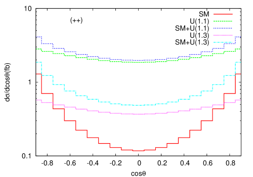
Figure 5: The angular distribution for SM, and SM+${\cal U}$ cross sections with the polarization configuration $(++)$. Here, we assume $\lambda_{0}/\Lambda_{U}=0.3$ TeV^-1, $d=1.1$ and $d=1.3$ at $\sqrt{s_{ee}}=1$ TeV.

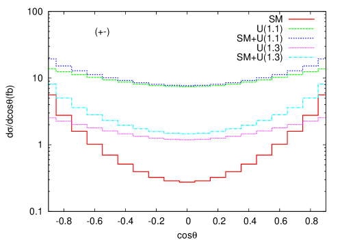
Figure 6: The angular distribution for SM, and SM+${\cal U}$ cross sections with the polarization configuration $(+-)$. Here, we assume $\lambda_{0}/\Lambda_{U}=0.3$ TeV^-1, $d=1.1$ and $d=1.3$ at $\sqrt{s_{ee}}=1$ TeV.

where $\delta{d\sigma\over d\cos\theta}$ is the error on the measurement. For one sided chi-square analysis, we assume $\chi^{2}\geq 2.7$, and we take two possible luminosity values, ${\cal L}=100fb^{-1}$, and ${\cal L}=1000fb^{-1}$ per year. We calculate the upper limits on the coupling of scalar unparticles by performing a fit to binned photon angular distribution as shown in Fig. 5 and 6. For the signal and background calculation, we take into account only the statistical error on the SM distribution. However, the systematic errors should be considered including $e^{+}/e^{-}$ beam conversion, the photon-photon collisions and the detector effects for the detection of photons, if they are controlled well the limits can be improved and benefitted from the advantage of high luminosity. Our limits on $\lambda_{0}$ are presented in the Table 1, and Table 2 for two polarization configurations.

Table 1: Upper limits on the $\lambda_{0}$ for the polarization configuration(++) for ${\cal L}=100(1000)$ fb^-1 and $\Lambda_{U}=1000$ GeV.

$\sqrt{s}$ GeV	d=1.01	d=1.1	d=1.3	d=1.5	d=1.7	d=1.9
500	$0.0865(0.065)$	$0.113(0.085)$	$0.194(0.1455)$	$0.316(0.237)$	$0.479(0.359)$	$0.551(0.413)$
1000	$0.0605(0.0455)$	$0.0745(0.056)$	$0.1115(0.0835)$	$0.1585(0.1185)$	$0.2095(0.157)$	$0.2105(0.1575)$
3000	$0.0300(0.0225)$	$0.0335(0.0250)$	$0.0403(0.030)$	$0.0458(0.0345)$	$0.0485(0.0365)$	$0.0393(0.0295)$
5000	$0.0213(0.016)$	$0.0225(0.017)$	$0.0245(0.0185)$	$0.0253(0.019)$	$0.0243(0.0183)$	$0.0178(0.0133)$

Table 2: Upper limits on the $\lambda_{0}$ for the polarization configuration(+-) for ${\cal L}=100(1000)$ fb^-1 and $\Lambda_{U}=1000$ GeV.

$\sqrt{s}$ GeV	d=1.01	d=1.1	d=1.3	d=1.5	d=1.7	d=1.9
500	$0.069(0.052)$	$0.091(0.0685)$	$0.1625(0.122)$	$0.2765(0.2075)$	$0.432(0.324)$	$0.504(0.378)$
1000	$0.0478(0.0358)$	$0.0593(0.0443)$	$0.0925(0.0695)$	$0.1375(0.1033)$	$0.1875(0.1408)$	$0.1915(0.1435)$
3000	$0.0235(0.0178)$	$0.0265(0.0198)$	$0.0333(0.0250)$	$0.0398(0.0298)$	$0.0435(0.0328)$	$0.0358(0.0268)$
5000	$0.0165(0.0125)$	$0.018(0.0135)$	$0.0205(0.0153)$	$0.022(0.0165)$	$0.0218(0.0163)$	$0.0165(0.0123)$

Since the the cross section is proportional with the $\lambda_{0}^{4}/\Lambda_{\cal U}^{4d}$, our limits can be restated regarding the corresponding behaviors of $\lambda_{0}$, and $\Lambda_{\cal U}$. In Figure 7 and 8, for the polarization configuration $(++)$ and $(+-)$, we plot the corresponding behaviors of $\Lambda_{U}$ and $\lambda_{0}$. Right hand side of each curve is ruled out according to the $95\%$C.L. analysis. For the analysis schemes discussed above the similar results can easily be obtained for the other center of mass energies with low/high luminosities.

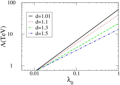
Figure 7: Upper limits on the scalar unparticle coupling $\lambda_{0}$ depending on $\Lambda_{\cal U}$ for (++) polarization at CLIC 5 TeV energy.

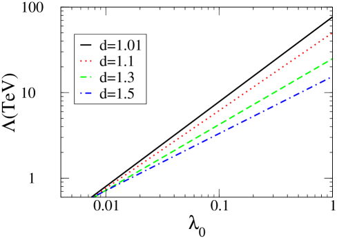
Figure 8: Upper limits on the scalar unparticle coupling $\lambda_{0}$ depending on $\Lambda_{\cal U}$ for (+-) polarization at CLIC 5 TeV energy.

In conclusion, for different values of the scaling dimension $d$, we put upper limits on $\lambda_{0}$ assuming the scalar unparticle effects on the polarized cross section can be distinguished from the SM contribution at $95\%$C.L. In our analysis, we consider the multi-TeV CLIC electron-positron collider, which will be launched at the CERN, for the center of mass energies $\sqrt{s}=0.5$ TeV-$5.0$ TeV, and the luminosities ${\cal L}=100fb^{-1}$, and ${\cal L}=1000fb^{-1}$ per year. Our calculations show that the limits on $\lambda_{0}$ get more stringent as one increases the luminosity and the center of mass energy of the collider. Our limits are consistent with the limits calculated from other low and high energy physics implications, for example Anchordoqui:2007dp ; Balantekin:2007eg .

Appendix A

A.1 1-loop SM Amplitudes

The lowest order SM contributions to the $\gamma\gamma\to\gamma\gamma$ process are 1-loop contributions of the charged fermions, and $W^{\pm}$ bosons. There are 16 helicity amplitudes contributing at the 1-loop level, and only three of them can be stated independently. We can choose them $(++++),(+++-)$, and $(++--)$. In the limits, $s,|t|,|u|>>M_{W}^{2}$, the only significant contributions come from $(++++)$ polarization configuration, and that can be expressed in the following form, Ref.Jikia:1993tc ; gounaris1999 . For the W boson contribution,

$$\frac{M_{++++}^{(W)}(\hat{s},\hat{t},\hat{u})}{\alpha^{2}} \approx 12+12\left(\frac{\hat{u}-\hat{t}}{\hat{s}}\right)\left[\ln\left(\frac{-\hat{u}-i\epsilon}{m_{W}^{2}}\right)-\ln\left(\frac{-\hat{t}-i\epsilon}{m_{W}^{2}}\right)\right]$$ (11)

$$+16\left(1-\frac{3\hat{t}\hat{u}}{4\hat{s}^{2}}\right)\left\{\left[\ln\left(\frac{-\hat{u}-i\epsilon}{m_{W}^{2}}\right)-\ln\left(\frac{-\hat{t}-i\epsilon}{m_{W}^{2}}\right)\right]^{2}+\pi^{2}\right\}$$

$$+16\hat{s}^{2}\left[\frac{1}{\hat{s}\hat{t}}\ln\left(\frac{-\hat{s}-i\epsilon}{m_{W}^{2}}\right)\ln\left(\frac{-\hat{t}-i\epsilon}{m_{W}^{2}}\right)+\frac{1}{\hat{s}\hat{u}}\ln\left(\frac{-\hat{s}-i\epsilon}{m_{W}^{2}}\right)\ln\left(\frac{-\hat{u}-i\epsilon}{m_{W}^{2}}\right)\right]$$

$$+\frac{16\hat{s}^{2}}{\hat{t}\hat{u}}\ln\left(\frac{-\hat{t}-i\epsilon}{m_{W}^{2}}\right)\ln\left(\frac{-\hat{u}-i\epsilon}{m_{W}^{2}}\right)$$

for the fermion loop,

$$\frac{M_{++++}^{(f)}(\hat{s},\hat{t},\hat{u})}{\alpha^{2}Q_{f}^{4}} \approx -8-8\left(\frac{\hat{u}-\hat{t}}{\hat{s}}\right)\left[\ln\left(\frac{-\hat{u}-i\epsilon}{m_{f}^{2}}\right)-\ln\left(\frac{-\hat{t}-i\epsilon}{m_{f}^{2}}\right)\right]$$ (12)

$$-4\left(\frac{\hat{t}^{2}+u^{2}}{s^{2}}\right)\left\{\left[\ln\left(\frac{-\hat{u}-i\epsilon}{m_{f}^{2}}\right)-\ln\left(\frac{-\hat{t}-i\epsilon}{m_{f}^{2}}\right)\right]^{2}+\pi^{2}\right\}$$

where $Q_{f}$ is the fermion charge, $m_{f}$ is the mass of the fermion, and for the helicity amplitudes we use $M_{h_{1}h_{2}h_{3}h_{4}}$ with the photon helicities $h_{i}=\pm$. Using the assumptions given in gounaris1999 , the other significant helicity amplitudes can be generated by using the relations $M_{+-+-}(\hat{s},\hat{t},\hat{u})=M_{++++}(\hat{u},\hat{t},\hat{s})$ and $M_{+--+}(\hat{s},\hat{t},\hat{u})=M_{+-+-}(\hat{s},\hat{u},\hat{t})$.

A.2 Expressions for unparticle contributions

In the calculations, we assume the following center of mass reference frame kinematical relations

$$p_{1}^{\mu}= E(1,0,0,1),\quad p_{2}^{\mu}=E(1,0,0,-1)$$ (13)

$$p_{3}^{\mu}= E(1,\sin\theta,0,\cos\theta),\quad p_{4}^{\mu}=E(1,-\sin\theta,0,-\cos\theta)$$ (14)

$$\epsilon_{1}^{\mu}= -\frac{1}{\sqrt{2}}(0,h_{1},i,0)\quad\epsilon_{2}^{\mu}=\frac{1}{\sqrt{2}}(0,-h_{2},i,0)$$ (15)

where $\epsilon_{1}\equiv\epsilon_{1}(h_{1}),\epsilon_{2}\equiv\epsilon_{1}(h_{2})$, etc., $h_{1},h_{2}=\{+,-\}$ stand for the polarizations, and we assume that the summation is over the final state polarizations.

Therefore, one can find the following terms

$$|M^{s}_{{\cal U}_{S}}(++)|^{2}= |M^{s}_{{\cal U}_{S}}(--)|^{2}=\frac{1}{8}[f(d)]^{2}[s]^{2d}$$ (16)

$$|M^{s}_{{\cal U}_{S}}(+-)|^{2}= |M^{s}_{{\cal U}_{S}}(-+)|^{2}=0$$ (17)

$$|M^{t}_{{\cal U}_{S}}(++)|^{2}= |M^{t}_{{\cal U}_{S}}(+-)|^{2}=|M^{t}_{{\cal U}_{S}}(-+)|^{2}=|M^{t}_{{\cal U}_{S}}(--)|^{2}=\frac{1}{16}[f(d)]^{2}[-t]^{2d}$$ (18)

$$|M^{u}_{{\cal U}_{S}}(++)|^{2}= |M^{u}_{{\cal U}_{S}}(+-)|^{2}=|M^{u}_{{\cal U}_{S}}(-+)|^{2}=|M^{u}_{{\cal U}_{S}}(--)|^{2}=\frac{1}{16}[f(d)]^{2}[-u]^{2d}$$ (19)

The phase exp$(-id\pi)$ associates with the $s-t$ and $s-u$ channel interferences

$$2{\cal R}e({M^{s}}^{*}_{{\cal U}_{S}}{M^{t}}_{{\cal U}_{S}})(++)= 2{\cal R}e({M^{s}}^{*}_{{\cal U}_{S}}{M^{t}}_{{\cal U}_{S}})(--)=\frac{1}{8}[f(d)]^{2}[s]^{d}[-t]^{d}\cos(d\pi)$$ (20)

$$2{\cal R}e({M^{s}}^{*}_{{\cal U}_{S}}{M^{t}}_{{\cal U}_{S}})(+-)= 2{\cal R}e({M^{s}}^{*}_{{\cal U}_{S}}{M^{t}}_{{\cal U}_{S}})(-+)=0$$ (21)

$$2{\cal R}e({M^{s}}^{*}_{{\cal U}_{S}}{M^{u}}_{{\cal U}_{S}})(++)= 2{\cal R}e({M^{s}}^{*}_{{\cal U}_{S}}{M^{u}}_{{\cal U}_{S}})(--)=\frac{1}{8}[f(d)]^{2}[s]^{d}[-u]^{d}\cos(d\pi)$$ (22)

$$2{\cal R}e({M^{s}}^{*}_{{\cal U}_{S}}{M^{u}}_{{\cal U}_{S}})(+-)= 2{\cal R}e({M^{s}}^{*}_{{\cal U}_{S}}{M^{u}}_{{\cal U}_{S}})(-+)=0$$ (23)

$$2{\cal R}e({M^{t}}^{*}_{{\cal U}_{S}}{M^{u}}_{{\cal U}_{S}})(++)= 2{\cal R}e({M^{t}}^{*}_{{\cal U}_{S}}{M^{u}}_{{\cal U}_{S}})(--)=\frac{1}{8}[f(d)]^{2}[tu]^{d}$$ (24)

$$2{\cal R}e({M^{t}}^{*}_{{\cal U}_{S}}{M^{u}}_{{\cal U}_{S}})(+-)= 2{\cal R}e({M^{t}}^{*}_{{\cal U}_{S}}{M^{u}}_{{\cal U}_{S}})(-+)=0$$ (25)

where

$$f(d)=\frac{8{\lambda_{0}^{2}}A_{d}}{\Lambda^{2d}\sin(d\pi)},$$ (26)

After the first version of this paper appeared online, similar works have been appeared, Chang:2008mk ; Kikuchi:2008pr . Our revised equations including the unparticle phase are in agreement with those papers. If one takes average over the squared helicity amplitudes then gets

$$|\bar{M}|^{2}=\frac{1}{4}[f(d)]^{2}\big{\{}[s]^{2d}+[-t]^{2d}+[-u]^{2d}+[tu]^{d}+\big{(}[s]^{d}[-t]^{d}+[s]^{d}[-u]^{d}\big{)}\cos(d\pi)\big{\}}.$$ (27)

A.3 Polarization Functions

Let $h_{e}$ and $h_{l}$ be the polarizations of the electron beam and the laser photon beam, respectively. According to Ginzburg:1983 , following function can be defined

$$C(x)=\frac{1}{1-x}+1-x-4r(1-r)-h_{e}h_{l}rz(2r-1)(2-x)$$ (28)

where $r=\frac{x}{z(1-x)}$, and $z=4E_{e}E_{l}/m_{e}^{2}$ describes the laser photon energy. Therefore, the photon number density is given by

$$f(x,h_{e},h_{l},z)=\big{(}\frac{2\pi\alpha^{2}}{m_{e}^{2}z\sigma_{c}}\big{)}C(x)$$ (29)

where

$$\sigma_{c}= \big{(}\frac{2\pi\alpha^{2}}{m_{e}^{2}z}\big{)}\big{[}\big{(}1-\frac{4}{z}-\frac{8}{z^{2}}\big{)}ln(z+1)+\frac{1}{2}+\frac{8}{z}-+\frac{1}{2(z+1)^{2}}\big{]}$$ (30)

$$+h_{e}h_{l}\big{(}\frac{2\pi\alpha^{2}}{m_{e}^{2}z}\big{)}\big{[}\big{(}1+\frac{2}{z}\big{)}ln(z+1)-\frac{5}{2}+\frac{1}{z+1}-\frac{1}{2(z+1)^{2}}\big{]}$$

The average helicity is given by

$$h_{\gamma}(x,h_{e},h_{l},z)=\frac{1}{C(x)}\big{\{}h_{e}\big{[}\frac{x}{1-x}+x(2r-1)^{2}\big{]}-h_{l}(2r-1)\big{(}1-x+\frac{1}{1-x}\big{)}\big{\}}$$ (31)

References

- (1) H. Georgi, Phys. Rev. Lett. 98, 221601 (2007) [arXiv:hep-ph/0703260].
- (2) T. Banks and A. Zaks, Nucl. Phys. B 196, 189 (1982).
- (3) H. Georgi, Phys. Lett. B 650, 275 (2007) [arXiv:0704.2457 [hep-ph]].
- (4) K. Cheung, W. Y. Keung and T. C. Yuan, Phys. Rev. Lett. 99, 051803 (2007) arXiv:0704.2588 [hep-ph]; Phys. Rev. D 76, 055003 (2007) [arXiv:0706.3155 [hep-ph]].
- (5) L. Anchordoqui and H. Goldberg, arXiv:0709.0678 [hep-ph].
- (6) A. B. Balantekin and K. O. Ozansoy, Phys. Rev. D 76 (2007) 095014 [arXiv:0710.0028 [hep-ph]].
- (7) C. F. Chang, K. Cheung and T. C. Yuan, arXiv:0801.2843 [hep-ph].
- (8) T. Kikuchi, N. Okada and M. Takeuchi, arXiv:0801.0018 [hep-ph].
- (9) E. Accomando et al. [CLIC Physics Working Group], arXiv:hep-ph/0412251. J. A. Aguilar-Saavedra et al. [ECFA/DESY LC Physics Working Group], arXiv:hep-ph/0106315. R. W. Assmann et al., A 3-TeV e+ e- linear collider based on CLIC technology, CERN-2000-008, Geneva, 2000. R. W. Assmann et al., CLIC contribution to the technical review committee on a 500 GeV linear collider, CERN-2003-007, Geneva, 2003. A. De Roeck, arXiv:hep-ph/0311138.
- (10) I. F. Ginzburg, G. L. Kotkin, V. G. Serbo and V. I. Telnov, Nucl. Instrum. Meth. 205 (1983) 47. I. F. Ginzburg, G. L. Kotkin, S. L. Panfil, V. G. Serbo and V. I. Telnov, Nucl. Instrum. Meth. A 219, 5 (1984).
- (11) S. Dawson and M. Oreglia, Ann. Rev. Nucl. Part. Sci. 54, 269 (2004) [arXiv:hep-ph/0403015].
- (12) G. Jikia and A. Tkabladze, Phys. Lett. B 323 (1994) 453 [arXiv:hep-ph/9312228].
- (13) G. J. Gounaris, P. I. Porfyriadis and F. M. Renard, Eur. Phys. J. C 9 (1999) 673 [arXiv:hep-ph/9902230]. ;Phys. Lett. B, 452, 76(1999)
- (14) K. m. Cheung, Phys. Rev. D 61 (2000) 015005 [arXiv:hep-ph/9904266].
- (15) H. Davoudiasl, Phys. Rev. D 60, 084022 (1999) [arXiv:hep-ph/9904425].
- (16) J. L. Hewett, F. J. Petriello and T. G. Rizzo, Phys. Rev. D 64 (2001) 075012 [arXiv:hep-ph/0010354].
- (17) P. J. Fox, A. Rajaraman and Y. Shirman, Phys. Rev. D 76 (2007) 075004 [arXiv:0705.3092 [hep-ph]].
- (18) B. Grinstein, K. Intriligator and I. Z. Rothstein, arXiv:0801.1140 [hep-ph].
- (19) W. M. Yao et al. [Particle Data Group], J. Phys. G 33, 1 (2006).