Improved Collaborative Filtering Algorithm via Information Transformation

Abstract

In this paper, we propose a spreading activation approach for collaborative filtering (SA-CF). By using the opinion spreading process, the similarity between any users can be obtained. The algorithm has remarkably higher accuracy than the standard collaborative filtering (CF) using Pearson correlation. Furthermore, we introduce a free parameter $\beta$ to regulate the contributions of objects to user-user correlations. The numerical results indicate that decreasing the influence of popular objects can further improve the algorithmic accuracy and personality. We argue that a better algorithm should simultaneously require less computation and generate higher accuracy. Accordingly, we further propose an algorithm involving only the top-$N$ similar neighbors for each target user, which has both less computational complexity and higher algorithmic accuracy.

PACS Nos.: 89.75.Hc, 87.23.Ge, 05.70.Ln

1 Introduction

With the advent of the Internet, the exponential growth of the World-Wide-Web and routers confront people with an information overload [1]. We are facing too much data to be able to effectively filter out the pieces of information that are most appropriate for us. A promising way is to provide personal recommendations to filter out the information. Recommendation systems use the opinions of users to help them more effectively identify content of interest from a potentially overwhelming set of choices [2]. Motivated by the practical significance to the e-commerce and society, various kinds of algorithms have been proposed, such as correlation-based methods [3, 4], content-based methods [5, 6], the spectral analysis [7, 8], principle component analysis [9], network-based methods [10, 11, 12, 13], and so on. For a review of current progress, see Ref. [14] and the references therein.

One of the most successful technologies for recommendation systems, called collaborative filtering (CF), has been developed and extensively investigated over the past decade [3, 4, 15]. When predicting the potential interests of a given user, such approach first identifies a set of similar users from the past records and then makes a prediction based on the weighted combination of those similar users’ opinions. Despite its wide applications, collaborative filtering suffers from several major limitations including system scalability and accuracy [16]. Recently, some physical dynamics, including mass diffusion [12, 11], heat conduction [10] and trust-based model [17], have found their applications in personal recommendations. These physical approaches have been demonstrated to be of both high accuracy and low computational complexity [10, 12, 11]. However, the algorithmic accuracy and computational complexity may be very sensitive to the statistics of data sets. For example, the algorithm presented in Ref. [12] runs much faster than standard CF if the number of users is much larger than that of objects, while when the number of objects is huge, the advantage of this algorithm vanishes because its complexity is mainly determined by the number of objects (see Ref. [12] for details). In order to increase the system scalability and accuracy of standard CF, we introduce a network-based recommendation algorithm with spreading activation, namely SA-CF. In addition, two free parameters, $\beta$ and $N$ are presented to increase the accuracy and personality.

2 Method

Denoting the object set as $O=\{o_{1},o_{2},\cdots,o_{n}\}$ and user set as $U$ = $\{u_{1},u_{2},$ $\cdots,$ $u_{m}\}$, a recommendation system can be fully described by an adjacent matrix $A=\{a_{ij}\}\in R^{n,m}$, where $a_{ij}=1$ if $o_{i}$ is collected by $u_{j}$, and $a_{ij}=0$ otherwise. For a given user, a recommendation algorithm generates a ranking of all the objects he/she has not collected before.

Based on the user-object matrix $A$, a user similarity network can be constructed, where each node represents a user, and two users are connected if and only if they have collected at least one common object. In the standard CF, the similarity between $u_{i}$ and $u_{j}$ can be evaluated directly by a correlation function:

$$s_{ij}^{c}=\frac{\sum_{l=1}^{n}a_{li}a_{lj}}{\min\{k(u_{i}),k(u_{j})\}},$$ (1)

where $k(u_{i})=\sum_{l=1}^{n}a_{li}$ is the degree of user $u_{i}$. Inspired by the diffusion process presented by Zhou et al. [12], we assume a certain amount of resource (e.g. recommendation power) is associated with each user, and the weight $s_{ij}$ represents the proportion of the resource, which $u_{j}$ would like to distribute to $u_{i}$. Following a network-based resource-allocation process [18] where each user distributes his/her initial resource equally to all the objects he/she has collected, and then each object sends back what it has received to all the users collected it, the weight $s_{ij}$ (the fraction of initial resource $u_{j}$ eventually gives to $u_{i}$) can be expressed as:

$$s_{ij}=\frac{1}{k(u_{j})}\sum^{n}_{l=1}\frac{a_{li}a_{lj}}{k(o_{l})},$$ (2)

where $k(o_{l})=\sum^{m}_{i=1}a_{li}$ denotes the degree object $o_{l}$. Using the spreading process, the user correlation network can be constructed, whose edge weight is obtained by Eq. (2). For the user-object pair $(u_{i},o_{j})$, if $u_{i}$ has not yet collected $o_{j}$ (i.e. $a_{ji}=0$), the predicted score, $v_{ij}$, is given as

$$v_{ij}=\frac{\sum_{l=1,l\neq i}^{m}s_{li}a_{jl}}{\sum_{l=1,l\neq i}^{m}s_{li}}.$$ (3)

From the definition of Eq.(3), one can get that, to a target user, all of his neighbors’ collection information would affect the recommendation results, which is different with the definition reachability [20]. Based on the definitions of $s_{ij}$ and $v_{ij}$, SA-CF can be given. The framework of the algorithm is organized as follows: (I) Calculate the user similarity matrix $\{s_{ij}\}$ based on the spreading approach; (II) For each user $i$, obtain the score $v_{ij}$ on every object not being yet collected by $j$; (III) Sort the uncollected objects in descending order of $v_{ij}$, and those in the top will be recommended.

3 Numerical results

To test the algorithmic accuracy and personality, we use a benchmark data-set, namely MovieLens [19]. The data consists of 1682 movies (objects) and 943 users, who vote movies using discrete ratings 1-5. Hence we applied the coarse-graining method previously used in Refs. [12, 13]: A movie is set to be collected by a user only if the giving rating is larger than 2. The original data contains $10^{5}$ ratings, 85.25% of which are $\geq 3$, thus the user-object (user-movie) bipartite network after the coarse gaining contains 85250 edges. To test the recommendation algorithms, the data set is randomly divided into two parts: the training set contains 90% of the data, and the remaining 10% of data constitutes the probe. The training set is treated as known information, while no information in the probe set is allowed to be used for prediction.

A recommendation algorithm should provide each user with an ordered queue of all its uncollected objects. It should be emphasized that, the length of queue should not be given artificially, because of the fact that the number of uncollected movies for different users are different. For an arbitrary user $u_{i}$, if the relation $u_{i}$-$o_{j}$ is in the probe set (according to the training set, $o_{j}$ is an uncollected object for $u_{i}$), we measure the position of $o_{j}$ in the ordered queue. For example, if there are $L_{i}=100$ uncollected movies for $u_{i}$, and $o_{j}$ is the 10th from the top, we say the position of $o_{j}$ is $10/L_{i}$, denoted by $r_{ij}=0.1$. Since the probe entries are actually collected by users, a good algorithm is expected to give high recommendations to them, thus leading to small $r_{ij}$. Therefore, the mean value of the position $r_{ij}$, $\langle r\rangle$ (called ranking score [12]), averaged over all the entries in the probe, can be used to evaluate the algorithmic accuracy: the smaller the ranking score, the higher the algorithmic accuracy, and vice verse. Implementing the SA-CF and CF [21], the average value of ranking score are $0.12187\pm 0.02406$ and $0.13069\pm 0.0571$ [22]. Clearly, under the simplest initial configuration, subject to the algorithmic accuracy, the SA-CF algorithm outperforms the standard CF.

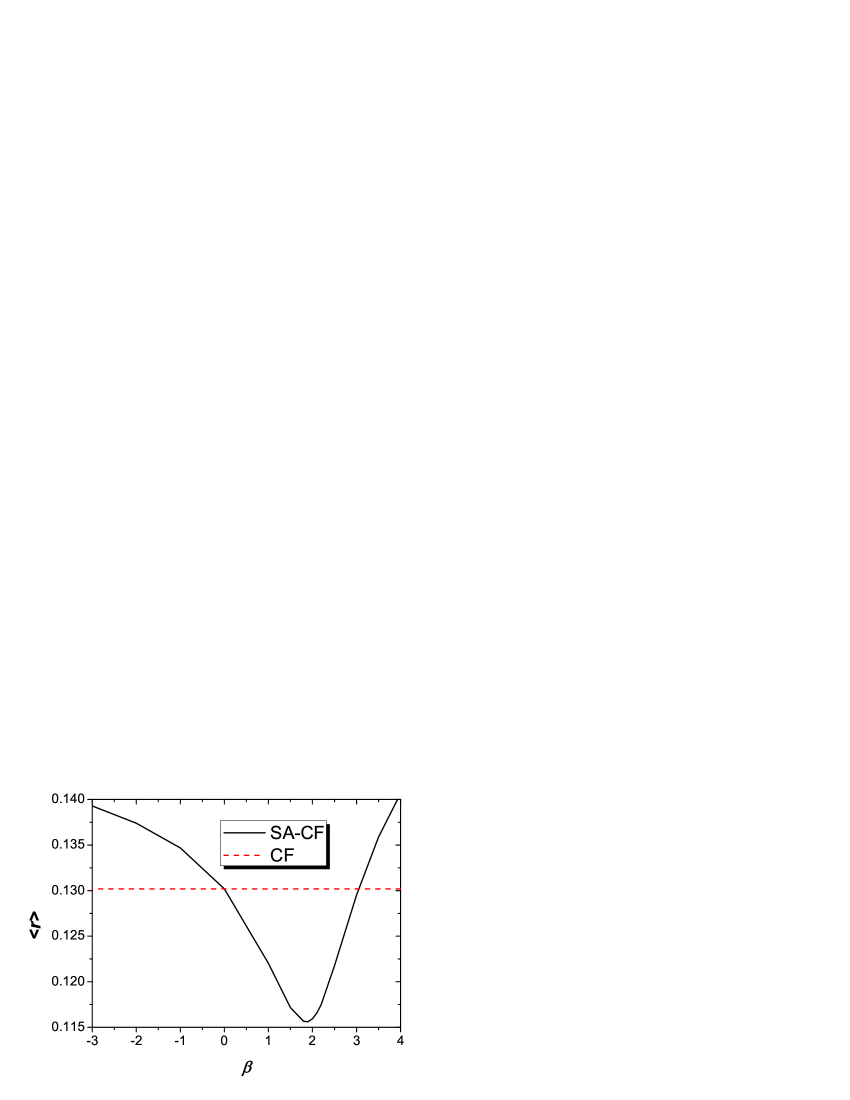
Figure 1: (Color online) $\langle r\rangle$ vs. $\beta$. The black solid and red dash curves represent the performances of SA-CF and CF, respectively. All the data points are obtained by averaging over ten independent runs with different data-set divisions.

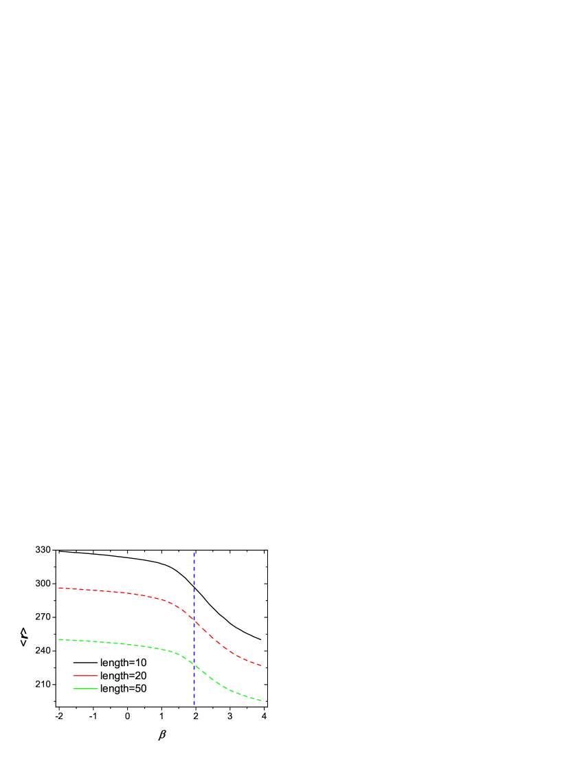
Figure 2: (Color online) The average degree of all recommended movies $\langle k\rangle$ vs. $\beta$. The black solid, red dashed and green dotted curves represent the cases with typical length $L=10,20$ and 50, respectively. The blue dot line corresponds to the optimal value $\beta_{\rm opt}=0.19$. All the data points are obtained by averaging over ten independent runs with different data-set divisions.

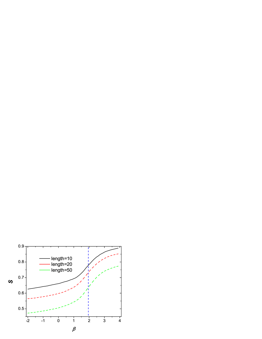
Figure 3: (Color online) $S$ vs. $\beta$. The black solid, red dashed and green dotted curves represent the cases with typical lengths $L=10,20$ and 50, respectively. The blue dot line corresponds to the optimal value $\beta_{\rm opt}=0.19$. All the data points are obtained by averaging over ten independent runs with different data-set divisions.

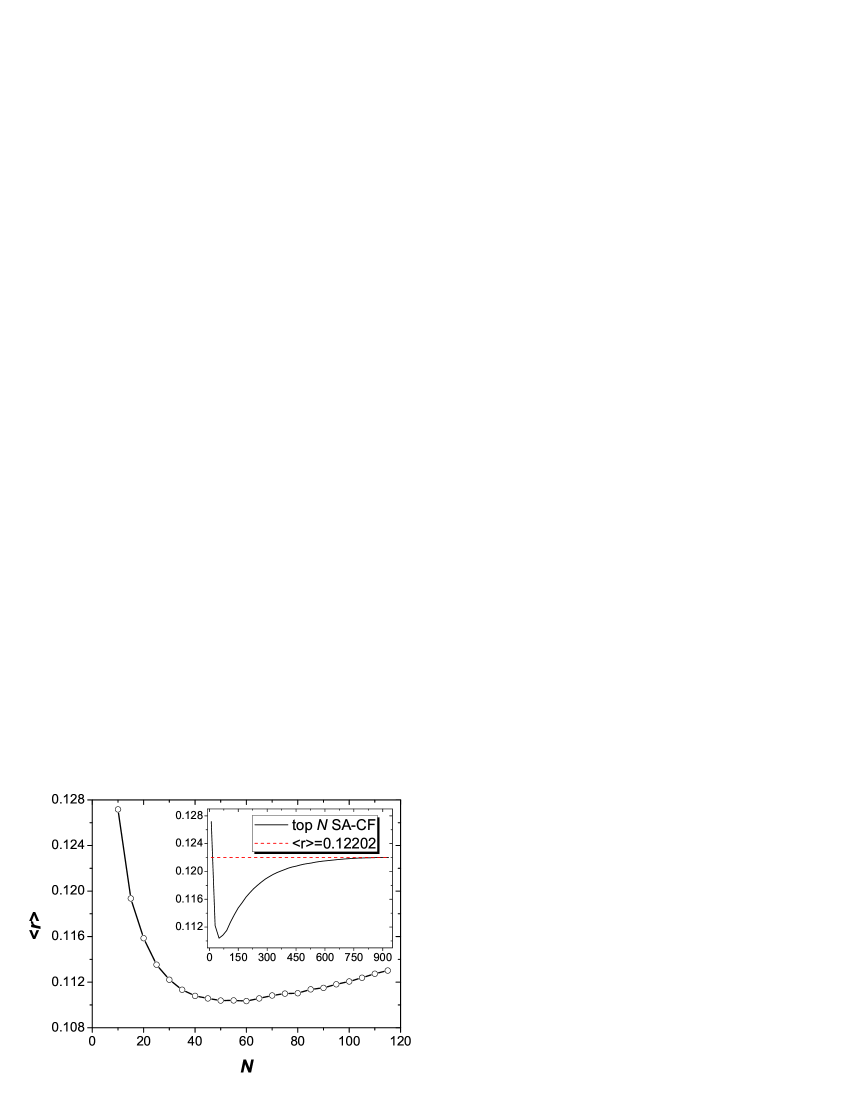
Figure 4: $\langle r\rangle$ vs. $N$. The inset shows the relation for larger $N$. Clearly, when $N$ approaches $n$, the algorithmic accuracy is the same as that of the SA-CF with $\langle r\rangle=0.12187\pm 0.02406$. All the data points are obtained by averaging over ten independent runs with different data-set divisions.

4 Two modified algorithms

In order to further improve the algorithmic accuracy, we propose two modified methods. Similar to the Ref. [13], taking into account the potential role of object degree may give better performance. Accordingly, instead of Eq. (2), we introduce a more complicated way to get user-user correlation:

$$s_{ij}=\frac{1}{k(u_{j})}\sum^{m}_{l=1}\frac{a_{li}a_{lj}}{k^{\beta}(o_{l})},$$ (4)

where $\beta$ is a tunable parameter. When $\beta=1$, this method degenerates to the algorithm mentioned in the last section. The case with $\beta>1$ weakens the contribution of large-degree objects to the user-user correlation, while $\beta<1$ will enhance the contribution of large-degree objects. According to our daily experience, if two users $u_{i}$ and $u_{j}$ has simultaneously collected a very popular object (with very large degree), it doesn’t mean that their interests are similar; on the contrary, if two users both collected an unpopular object (with very small degree), it is very likely that they share some common and particular tastes. Therefore, we expect a larger $\beta$ (i.e. $\beta>1$) will lead to higher accuracy than the routine case $\beta=1$.

Fig.1 reports the algorithmic accuracy as a function of $\beta$. The curve has a clear minimum around $\beta=1.9$, which strongly support the above statement. Compared with the routine case ($\beta=1$), the ranking score can be further reduced by 11.2% at the optimal value. It is indeed a great improvement for recommendation algorithms. Besides accuracy, the average degree of all recommended movies $\langle k\rangle$ and the mean value of Hamming distance $S$ [13] are taken in account to measure the algorithmic personality. The movies with higher degrees are more popular than the ones with smaller degrees. The personal recommendation should give small $\langle k\rangle$ to fit the special tastes of different users. Fig.2 reports the average degree of all recommended movies as a function of $\beta$. One can see from fig.2 that the average degree is negatively correlated with $\beta$, thus depressing the recommendation power of high-degree objects gives more opportunity to the unpopular objects. The Hamming distance, $S=\langle H_{ij}\rangle$, is defined by the mean value among any two recommended lists of $u_{i}$ and $u_{j}$, where $H_{ij}=1-Q/L$, $L$ is the list length and $Q$ is the overlapped number of objects in the two users’ recommended lists. Fig.3 shows the positively correlation between $S$ and $\beta$, in according with the simulation results in fig.2, which indicates that depressing the influence of high-degree objects makes the recommendations more personal. The above simulation results indicate that SA-CF outperforms CF from the viewpoints of accuracy and personality.

Besides the algorithmic accuracy and personality, the computational complexity should also be taken into account. Actually, we argue that a better algorithm should simultaneously require less computation and generate higher accuracy. Note that, the computational complexity of Eq. (3) is very high if the number of user, $m$, is huge. Actually, the majority of user-user similarities are very small, which contribute little to the final recommendation. However, those inconsequential items, corresponding to the less similar users, dominate the computational time of Eq. (3). Therefore, we propose a modified algorithm, so-called top-$N$ SA-CF, which only considers the $N$ most similar users’ information to any given user. That is to say, in the top-$N$ SA-CF, the sum in Eq. (3) runs over only the $N$ most similar users of $u_{i}$. In the process of calculation the similarity matrix $s_{ij}$, to each other, we can simultaneously record its most similar users. When $m\gg N$, the additional computing time for top-$N$ similar users are remarkably shorter than what we can save from the traditional calculation of Eq. (3). More surprisingly, as shown in Fig.4, with properly chosen $N$, this algorithm not only reduces the computation, but also enhances the algorithmic accuracy. This property is of practical significance, especially for the huge-size recommender systems. From figures 2 and 3, one can find that, to the same $\beta$ range, the anticorrelations between $\langle k\rangle$, $S$ and $\beta$ are different in different $\beta$ range. Maybe there is a phase transition in the anticorrelations. Because this paper mainly focuses on the accuracy and personality of the recommendation algorithms, this issue would be investigated in the future.

5 Conclusions

In this paper, the spreading activation approach is presented to compute the user similarity of the collaborative filtering algorithm, named SA-CF. The basic SA-CF has obviously higher accuracy than the standard CF. Ignoring the degree-degree correlation in user-object relations, the algorithmic complexity of SA-CF is $\mathbb{O}(m\langle k_{u}\rangle\langle k_{o}\rangle+mn\langle k_{o}\rangle)$, where $\langle k_{u}\rangle$ and $\langle k_{o}\rangle$ denote the average degree of users and objects. Correspondingly, the algorithmic complexity of the standard CF is $\mathbb{O}(m^{2}\langle k_{u}\rangle+mn\langle k_{o}\rangle)$, where the first term accounts for the calculation of similarity between users, and the second term accounts for the calculation of the predictions. In reality, the number of users, $m$, is much larger than the average object degree, $\langle k_{o}\rangle$, therefore, the computational complexity of SA-CF is much less than that of the standard CF. The SA-CF has great potential significance in practice.

Furthermore, we proposed two modified algorithms based on SA-CF. The first algorithm weakens the contribution of large-degree objects to user-user correlations, and the second one eliminates the influence of less similar users. Both the two modified algorithm can further enhance the accuracy of SA-CF. More significantly, with properly choice of the parameter $N$, top-$N$ SA-CF can simultaneously reduces the computational complexity and improves the algorithmic accuracy.

A natural question on the presented algorithms is whether these algorithms are robust to other data-sets or random recommendation? To SA-CF, the answer is yes, because it would get the user similarity more accurately. While to the two modified algorithms, the answer is no. Since both of the two modified algorithms introduced the tunable parameters $\beta$ and $N$, the optimal values of different data-sets are different. The further work would focus on how to find an effective way to obtain the optimal value exactly, then the modified algorithms could be implemented more easily.

We are grateful to Tao Zhou, Zoltán Kuscsik, Yi-Cheng Zhang and Metú$\breve{s}$ Medo for their greatly useful discussions and suggestions. This work is partially supported by SBF (Switzerland) for financial support through project C05.0148 (Physics of Risk), the National Basic Research Program of China (973 Program No. 2006CB705500), the National Natural Science Foundation of China (Grant Nos. 60744003, 10635040, 10532060, 10472116), GQ was supported by the Liaoning Education Department (Grant No. 20060140).

References

- [1] A. Broder, R. Kumar, F. Moghoul, P. Raghavan, S. Rajagopalan, R. Stata, A. Tomkins, and J.Wiener, Comput. Netw. 33, 309 (2000).
- [2] P. Resnick and H. R. Varian, Commun. ACM 40, 56 (1997).
- [3] J. L. Herlocker, J. A. Konstan, K. Terveen, and J. T. Riedl, ACM Trans. Inform. Syst. 22, 5 (2004).
- [4] J. A. Konstan, B. N. Miller, D. Maltz, J. L. Herlocker, L. R. Gordon, and J. Riedl, Commun. ACM 40, 77 (1997).
- [5] M. Balabanović and Y. Shoham, Commun. ACM 40, 66 (1997).
- [6] M. J. Pazzani, Artif. Intell. Rev. 13, 393 (1999).
- [7] D. Billsus and M. Pazzani, Proc. Int’l Conf. Machine Learning (1998).
- [8] B. Sarwar, G. Karypis, J. Konstan, and J. Riedl, Proc. ACM WebKDD Workshop (2000).
- [9] K. Goldberg, T. Roeder, D. Gupta, and C. Perkins, Inform. Ret. 4, 133 (2001).
- [10] Y.-C. Zhang, M. Blattner, and Y.-K. Yu, Phys. Rev. Lett. 99, 154301 (2007).
- [11] Y.-C. Zhang, M. Medo, J. Ren, T. Zhou, T. Li, and F. Yang, EPL 80, 68003 (2007).
- [12] T. Zhou, J. Ren, M. Medo, and Y.-C. Zhang, Phys. Rev. E 76, 046115 (2007).
- [13] T. Zhou, L.-L. Jiang, R.-Q. Su, and Y.-C. Zhang, EPL 81, 58004 (2008).
- [14] G. Adomavicius and A. Tuzhilin, IEEE Trans. Know. & Data Eng. 17, 734 (2005).
- [15] Z. Huang, H. Chen, and D. Zeng, ACM Trans. Inform. Syst. 22, 116 (2004).
- [16] B. Sarwar, G. Karypis, J. Konstan, and J. Reidl, In Proceedings of the ACM Conference on Electronic Commerce. ACM, New York, 158 (2000).
- [17] F. W. Walter, S. Battiston, and F. Schweitzer, Auto. Agents and Multi-Agent Sys. 16(1), 1573 (2008).
- [18] Q. Ou, Y.-D. Jin, T. Zhou, B.-H. Wang, and B.-Q. Yin, Phys. Rev. E 75, 021102 (2007).
- [19] The MovieLens data can be downloaded from the web-site of GroupLens Research (http://www.grouplens.org).
- [20] P. G. Lind, L. R. da Silva, J. S. Andrade, and H. J. Herrmann, Phys. Rev. E 76, 036117 (2007).
- [21] The predicted results of standard CF can be directly obtained by applying Eq. (3) using instead of .
- [22] Note that, the ranking score of the standard CF reported here is slightly different from that of the Ref. [12]. It is because in this paper, if a movie in the probe set has not yet appeared in the known set, we automatically remove it from the probe; while the Ref. [12] takes into account those movies only appeared in the probe via assigning zero score to them. Another alterative way is to automatically move those movies from the probe set to the known set, which guarantees that any target movie in the probe set has been collected by at least one user in the known set. The values of are slightly different for these three implementations, however, the choice of different implementations has no substantial effect on our conclusions.