The Operator Product Expansion on the Lattice

Abstract:

We investigate the Operator Product Expansion (OPE) on the lattice by directly measuring the product $\langle J_{\mu}J_{\nu}\rangle$ (where $J$ is the vector current) and comparing it with the expectation values of bilinear operators. This will determine the Wilson coefficients in the OPE from lattice data, and so give an alternative to the conventional methods of renormalising lattice structure function calculations. It could also give us access to higher twist quantities such as the longitudinal structure function $F_{L}=F_{2}-2xF_{1}$. We use overlap fermions because of their improved chiral properties, which reduces the number of possible operator mixing coefficients.

1 Introduction

Our main theoretical tool for interpreting hadronic Deep Inelastic Scattering (DIS) is the Operator Product Expansion (OPE). This relates the experimentally measurable electromagnetic tensor $W_{\mu\nu}$,

$$W_{\mu\nu}(p,q)\equiv\langle\psi(p)|J_{\mu}(q)J^{\dagger}_{\nu}(q)|\psi(p)\rangle$$ (1)

to a sum over matrix elements of local operators.

$$W_{\mu\nu}(p,q)=\langle\psi(p)|J_{\mu}(q)J^{\dagger}_{\nu}(q)|\psi(p)\rangle=\sum_{m}C_{\mu\nu}^{m}(q)\langle\psi(p)|{\cal O}^{m}|\psi(p)\rangle\;.$$ (2)

The local operators have interpretations in terms of the target hadron’s internal structure.

In each term of the OPE the scales separate. Dependence on the photon scale $q$ is in the Wilson coefficient $C_{\mu\nu}^{m}(q)$ while dependence on the quark momentum $p$ is in the matrix element $\langle\psi(p)|{\cal O}^{m}|\psi(p)\rangle$.

There has been a long history of lattice calculations of the hadronic matrix elements which occur in the OPE, but the Wilson coefficients are usually calculated perturbatively. In this work we investigate the possibility of also calculating the Wilson coefficients on the lattice by looking at the product of two electromagnetic currents.

The Wilson coefficients are independent of the target. In our calculation we measure the current product (Compton amplitude) between quark states. We then plan to use the resulting Wilson coefficients together with lattice data on nucleon matrix elements to look at deep inelastic scattering.

If we can measure the coefficients accurately enough we could learn something about higher twist effects, and non-leading amplitudes such as the longitudinal structure function $F_{L}=F_{2}-2xF_{1}$. To calculate power corrections of this type we need to know both the matrix elements and the Wilson coefficients beyond perturbation theory [1].

In this work we report on an ongoing study of the lattice OPE using overlap fermions. These have the advantage of better chiral properties, which reduces the problems of operator mixing, and makes $O(a)$ improvement much simpler. Our earlier study using Wilson fermions was described in [2]

2 Symmetry

If $p\ll q$ we will be able to truncate our set of operators according to their dimension. The operators we consider are the quark bilinears with up to three derivatives. These are the operators $\overline{\psi}\Gamma\psi,\;\overline{\psi}\Gamma D_{\mu_{1}}\psi,\;\overline{\psi}\Gamma D_{\mu_{1}}D_{\mu_{2}}\psi,\;\overline{\psi}\Gamma D_{\mu_{1}}D_{\mu_{2}}D_{\mu_{3}}\psi$ where the matrix $\Gamma$ can be any of the 16 matrices in the Clifford algebra. This means that there are a total of $16\times(1+4+4^{2}+4^{3})=1360$ operators to consider. Do we need to find 1360 different $C^{m}$ values?

To reduce the number of independent coefficients we want to choose a $q$ vector with as much lattice symmetry as possible, so we have taken $q\propto(1,1,1,1)$. The data presented here are for the choice $aq=\left(\frac{\pi}{2},\frac{\pi}{2},\frac{\pi}{2},\frac{\pi}{2}\right)$.

In the expansion for $W_{44}$ we know that rotations and reflections that mix the space direction $x,y,z$ are symmetries. So it is obvious that the Wilson coefficients of $\overline{\psi}\gamma_{1}D_{1}\psi,\;\overline{\psi}\gamma_{2}D_{2}\psi$ and $\overline{\psi}\gamma_{3}D_{3}\psi$ should all be the same. Exploiting symmetry this way reduces the original $1360$ coefficients down to only $67$, a much more manageable problem. We can also use symmetries to relate different components of $W_{\mu\nu}$. For example, the Wilson coefficient of $\overline{\psi}\gamma_{4}D_{4}\psi$ in $W_{44}$ is the same as the $C$ for $\overline{\psi}\gamma_{3}D_{3}\psi$ in $W_{33}$.

3 Lattice Details

We are carrying out calculations with overlap valence fermions, due to their superior chiral properties. However because of the high cost of a full dynamical overlap calculation, we have to use gauge configurations calculated with $N_{f}=2$ dynamical clover fermions.

The overlap fermions are calculated with $\rho=1.5$ and bare mass $am=0.024$. The results discussed in this work used a $16^{3}\times 32$ lattice, simulated with $N_{f}=2$ clover fermions, at $\beta=5.29$ and $\kappa=0.1350$, which corresponds to a lattice spacing of $a=0.075fm$.

The Green’s functions have been $O(a)$ improved, which is easy to do with overlap fermions. The current $J_{\mu}(x)$ was represented by the local current $\overline{\psi}(x)\gamma_{\mu}\psi(x)$. Since we are measuring operators between quark states we have to fix the gauge. We used the lattice Landau gauge. We use a momentum source [3, 4] for all Greens functions, which leads to a great reduction in statistical noise.

We used a momentum transfer $aq=\left(\frac{\pi}{2},\frac{\pi}{2},\frac{\pi}{2},\frac{\pi}{2}\right)$ corresponding to $|q|=8.3GeV$. For this $q$ value we measured the two-point and three-point functions for 28 different $p$ vectors, with a large spread in directions. Here we give results for $\langle J_{4}J_{4}\rangle$, we are also collecting data on other components of the current-current tensor.

We only consider the flavour non-singlet case, so we do not include any purely gluonic operators in our calculation.

4 Strategy

We calculate the Compton scattering amplitude for a quark with a large number of $p$ values. The result is a Dirac matrix for each $p$ vector, i.e. 16 complex numbers. So our data on the Compton amplitude consist of $16M_{p}$ complex numbers. We also calculate the operator Greens functions for each of our operators, for all of these $p$ values. This gives $(16M_{p})\times N_{O}$ numbers as our data on the operators.

The information we want to extract from all this data are the $N_{O}$ Wilson coefficients which best reproduce the Compton scattering amplitudes.

This is essentially a linear algebra problem, and is best written as a matrix equation

$$W_{\mu\nu}(p_{i},q)=\sum_{m}\langle\psi(p_{i})|{\cal O}^{m}|\psi(p_{i})\rangle\;C_{\mu\nu}^{m}(q)$$ (3)

$$\left(\begin{array}[]{ccc}W^{p_{1}}\\ \vdots\\[-1.99997pt] \vdots\\ W^{p_{M}}\\ \end{array}\right)=\left(\begin{array}[]{ccc}O_{1}^{p_{1}}&\cdots&O_{N}^{p_{1}}\\ \vdots&&\vdots\\[-1.99997pt] \vdots&&\vdots\\ O_{1}^{p_{M}}&\cdots&O_{N}^{p_{M}}\\ \end{array}\right)\left(\begin{array}[]{ccc}C_{1}\\ \vdots\\ C_{N}\\ \end{array}\right)\;.$$ (4)

$$(16M_{p})\quad\qquad(16M_{p}\times N_{O})\cdot(N_{O})$$

5 Singular Value Decomposition (SVD)

There are two difficulties with this system of equations. Firstly if $16M_{p}>N_{O}$ the system is overdetermined, so no exact solution will be possible. Secondly, some of the operators might be linearly dependent, in which case the system is also ill-conditioned, and there will not even be a unique best approximation to the solution.

Nevertheless by using Singular Value Decomposition (SVD) [5], the standard technique for problems of this type, we can find values of the coefficients $C_{i}$ which give a very good, and very stable, approximate solution.

We can always factorise the operator matrix $O$ as

$$O = U\omega V^{T}$$ (5)

$$O_{i,j} = \sum_{k=1}^{N}U_{ik}\omega_{k}V_{jk}$$ (6)

where $U$ and $V$ are column-orthonormal, $U$ is $(16M_{p})\times N_{O}$, $V$ is $N_{O}\times N_{O}$ and $\omega$ is a diagonal $N_{O}\times N_{O}$ matrix, with positive real eigenvalues $\omega_{k}$ arranged in descending order. The $\omega_{k}$ are the analogues of eigenvalues for a rectangular matrix, while the matrices $U$ and $V$ contain the eigenvectors for the system. If some of the $\omega_{k}$ are very small they can safely be dropped from the sum without significantly changing $O$.

We define $O^{(n)}$ as the approximation to $O$ that we get by keeping the $n$ largest $\omega$ values, and dropping the $N-n$ smallest values. This gives

$$O^{(n)}_{i,j}=\sum_{k=1}^{n}U_{ik}\omega_{k}V_{jk}\equiv U^{(n)}\omega^{(n)}(V^{(n)})^{T}$$ (7)

where now $U^{(n)}$ is $(16M_{p})\times n$, $\omega^{(n)}$ is $n\times n$ and $V^{(n)}$ is $N_{O}\times n$. $O^{(n)}$ is still $(16M_{p})\times N_{O}$. It can be shown that the least-squares solution to $O^{(n)}C=W$ is $C=V^{(n)}(\omega^{(n)})^{-1}(U^{(n)})^{T}W$.

What singular value decomposition has done is to find the $N-n$ linear combinations of our original operators which have the least influence on $W$, and discarded those combinations. Discarding these operators makes the problem much more stable. However if we discard too many operators, $O^{(n)}$ will no longer be a good approximation to $O$, and so the solution of the approximate system will not give a good approximate solution to the true problem.

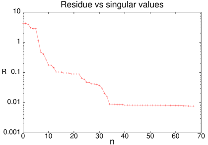
To solve a system by SVD we vary $n$, the number of $\omega_{k}$ values retained, looking for a region where the residue $R=(W-OC)^{2}$ is small and the system is stable. Fig.1 shows how the residue declines as the number of singular values is increased. A plateau is reached beyond $n\approx 40$. Beyond this point adding more operators does not decrease the residue significantly.

Figure 1: The residue of the fit as a function of $n$, the number of singular values retained.

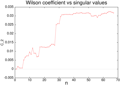
To judge the stability of the fit, we look at the value of one of the Wilson coefficients, and see how it depends on $n$. In Fig.2 we show the result for the choice $C_{2}$ in our list of operators, the operator $\overline{\psi}(\gamma_{1}D_{1}+\gamma_{2}D_{2}+\gamma_{3}D_{3})\psi$. At first the coefficient changes dramatically as operators are added, but by the time $n$ has reached 40, there are only minor changes. If $n$ is made too large, there is a risk that we will start “fitting to the noise”, and the value of the coefficient will become noisy. There are indeed some fluctuations beyond $n=50$, but they are not unduly large.

Figure 2: The value of $C_{2}$, the Wilson coefficient for ${\overline{\psi}}(\gamma_{1}{D}_{1}+\gamma_{2}{D}_{2}+\gamma_{3}{D}_{3})\psi$, as a function of $n$, the number of singular values retained.

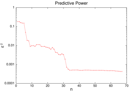
Another way of judging the quality of the fit is to exclude one momentum value from the fit, and see how well it is predicted by the data at all the other momentum values. The result is shown in Fig.3. Again we see that we need at least 40 singular values to produce a fit with good predictive power. If, at large $n$ we started fitting to the errors in the data, we would expect to see the predictive power becoming worse. There doesn’t seem to be any sign of this happening.

Figure 3: The accuracy with which the fit predicts the value of $W_{\mu\nu}$ as a function of $n$.

6 Results

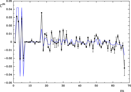
In Fig.4 we show the results of our fit. Chiral symmetry shows up well. Operator number 1, the operator $\overline{\psi}{\bf 1}\psi$, and operators 7 to 16, which are two-derivative operators proportional to the unit matrix or to $\sigma$ matrices, are ruled out by chiral symmetry, so they would have Wilson coefficients of 0 in the chiral limit. Here, using overlap fermions, we find that these coefficients are indeed small. This contrasts with earlier work with Wilson fermions, [2], [6], where the operator $\overline{\psi}{\bf 1}\psi$ was prominent.

Figure 4: The Wilson coefficients for $W^{44}$ determined on the lattice according to our procedure. They are compared with the lattice tree-level values, shown by the blue line.

We have calculated the tree-level Wilson coefficients for overlap fermions, following the calculation set out in [6]. The tree-level results are shown by the blue line in Fig.4. We see that the pattern of Wilson coefficients is very similar.

These results are at a single value of $|aq|$. We intend to gather data at other values to investigate the size of lattice artefacts, which should be $O(a^{2})$ for overlap fermions.

7 Conclusions

Using Singular Value Decomposition we have been able to reconstruct Wilson coefficients from lattice data on the electromagnetic tensor. Statistical errors are small, due to our use of momentum sources for the inversions.

The results we have look reasonable, they follow a pattern similar to that seen at tree-level, and they show the effects expected from chiral symmetry. So far we only have data from a rather large value of $|aq|$, we plan to look at more $q$ values to check for $O(a^{2})$ lattice errors.

8 Acknowledgements

The calculations for this work were carried out on an IBM pSeries 690 in Berlin, belonging to the HLRN.

References

- [1] G. Martinelli and C. T. Sachrajda, Nucl. Phys. B 478 (1996) 660 [arXiv:hep-ph/9605336].
- [2] S. Capitani, M. Göckeler, R. Horsley, H. Oelrich, D. Petters, P.E.L. Rakow and G. Schierholz, Nucl. Phys. Proc. Suppl. 73 (1999) 288 [arXiv:hep-lat/9809171].
- [3] M. Göckeler, R. Horsley, H. Oelrich, H. Perlt, P. Rakow, G. Schierholz and A. Schiller, Nucl. Phys. Proc. Suppl. 63 (1998) 868 [arXiv:hep-lat/9710052].
- [4] M. Göckeler, R. Horsley, H. Oelrich, H. Perlt, D. Petters, P.E.L. Rakow, A. Schäfer, G. Schierholz and A. Schiller, Nucl. Phys. B 544 (1999) 699 [arXiv:hep-lat/9807044].
- [5] W.H. Press S.A. Teukolsky, W.T. Vetterling and B.P. Flannery, Numerical Recipes, Cambridge University Press, Cambridge (1989).
- [6] M. Göckeler, R. Horsley, H. Perlt, P.E.L. Rakow, G. Schierholz and A. Schiller [QCDSF Collaboration], PoS LAT2006 (2006) 119 [arXiv:hep-lat/0610064].