The critical line from imaginary to real baryonic chemical potentials in two-color QCD

Abstract

The method of analytic continuation from imaginary to real chemical potentials $\mu$ is one of the few available techniques to study QCD at finite temperature and baryon density. One of its most appealing applications is the determination of the critical line for small $\mu$: we perform a direct test of the validity of the method in this case by studying two-color QCD, where the sign problem is absent. The (pseudo)critical line is found to be analytic around $\mu^{2}=0$, but a very large precision would be needed at imaginary $\mu$ to correctly predict the location of the critical line at real $\mu$.

I Introduction

The study of strong interactions at finite temperature and baryon density is relevant to fundamental phenomenological issues, like the experimental search for the deconfinement transition in heavy ion collisions or the properties of compact astrophysical objects. Several questions need to be clarified: the structure of the QCD phase diagram, i.e. the location and the nature of the transition lines, as well as the properties of strongly interacting matter, specially close to the transition lines. Unfortunately numerical lattice simulations, which are the ideal non-perturbative tool for first principle theoretical studies, are hindered in presence of a baryon chemical potential by the fermionic determinant being complex, which makes importance sampling techniques not usable.

Various possibilities have been explored to circumvent the problem: reweighting techniques glasgow ; fodor ; density , the use of an imaginary chemical potential either for analytic continuation muim ; immu_dl ; azcoiti ; chen ; giudice ; potts3d ; cea ; defor06 ; sqgp ; conradi ; cea1 ; kt or for reconstructing the canonical partition function rw ; cano1 ; cano2 , Taylor expansion techniques taylor1 ; taylor2 and non-relativistic expansions hmass1 ; hmass2 ; hmass3 . All these methods do not really solve the problem and are expected to work well in a limited range of parameters. Cross-checks among them and direct test of the methods in simpler models are therefore extremely important.

In the present paper we consider the method of analytic continuation. The fermionic determinant, which is complex in presence of a real baryonic chemical potential $\mu$, is instead real if $\mu$ is purely imaginary, making usual Monte Carlo simulations feasible. Due to CP invariance, the partition function $Z$ is an even function of $\mu$, $Z=Z(T,\mu^{2})$. Numerical results obtained at imaginary $\mu$’s ($\mu^{2}<0$) can be used to fit the behaviour of physical observables with suitable functions, which can then be continued to $\mu^{2}>0$. The method is expected to fail outside analyticity domains, hence in particular when crossing physical or unphysical transition lines; but numerical instabilities, strictly linked to the choice of interpolating functions, can be source of systematic errors also elsewhere. A model where numerical simulations are possible both at imaginary and real values of $\mu$ is the ideal testground to study such systematic effects and the general reliability of the method: an example is provided by two-color QCD, where various studies regarding the analytic continuation of physical observables have been performed in the past giudice ; cea ; cea1 .

One of the most important applications of analytic continuation is the determination of the critical line or of critical surfaces for small values of $\mu$ muim ; immu_dl ; azcoiti ; chen ; defor06 . The theoretical basis in this case is not as straightforward as for physical observables and is based on the assumption that susceptibilities, whose peaks signal the presence of the transition, be analytic functions of the parameters on a finite volume muim . Direct tests of the method are even more important in this case: therefore we extend our analysis of two-color QCD to the study of the (pseudo)critical line. As in usual QCD simulations, we will determine locations of the critical line for $\mu^{2}<0$ and interpolate them by suitable functions to be continued to $\mu^{2}>0$. The prediction obtained at real $\mu$ will then be compared with direct determinations of the transition line.

II Numerical results

As in Ref. cea , to which we refer for further details about our numerical setup, we have performed numerical simulations on a $16^{3}\times 4$ lattice of the SU(2) gauge theory with $n_{f}=8$ degenerate staggered fermions having mass $am=0.07$. The algorithm adopted has been the usual exact $\phi$ algorithm described in Ref. Gottlieb:1987mq , properly modified for the inclusion of a finite chemical potential. Simulations have been performed on the APE100 and APEmille crates in Bari and on the computer facilities at the INFN apeNEXT Computing Center in Rome.

Figure 1: Chiral susceptibility at $(a\mu)^{2}=-0.1225$ vs $\beta$.

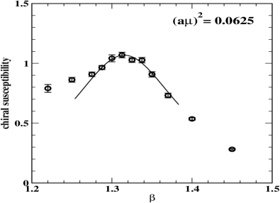
Figure 2: Chiral susceptibility at $(a\mu)^{2}=0.0625$ vs $\beta$.

In absence of true non-analyticities at the transition line, as on a finite volume, the location of the critical line may be dependent on the observable chosen to probe the transition. For that reason we have decided to determine, for a set of $\mu^{2}$ values, the critical couplings $\beta_{c}(\mu^{2})$ by looking at the peaks of the susceptibilities of three different observables: the chiral condensate, the Polyakov loop and the plaquette. We have taken the $\mu^{2}$ values on the imaginary side in the so-called first Roberge-Weiss (RW) sector, i.e. in the range delimited by $(a\mu)^{2}=-(\pi/8)^{2}$ and $\mu^{2}=0$ (see Ref. cea for a detailed discussion on the phase diagram in the $T-i\mu$ plane).

In Figs. 1 and 2 we show as examples the behavior with $\beta$ of the chiral susceptibility at $(a\mu)^{2}=-0.1225$ and $(a\mu)^{2}=0.0625$, respectively. In Table 1 we summarize our determinations of $\beta_{c}(\mu^{2})$, obtained by fitting the peaks of the susceptibilities according to a Lorentzian function. The values of $\beta_{c}(\mu^{2})$ depend very weakly on the “probe” observable; only in one case the relative deviation between two determinations at the same $\mu^{2}$ slightly exceeds 3$\sigma$.

We have tried at first to determine the critical line by interpolating the values of $\beta_{c}(\mu^{2})$ for $\mu^{2}\leq 0$ only, i.e. for the first seven entries in Table 1, and have repeated this procedure for each of the three observables considered.

Table 1: Summary of the critical values of $\beta$ obtained by fitting the peaks of the susceptibilities of chiral condensate $\langle\overline{\psi}\psi\rangle$, Polyakov loop $\langle L\rangle$ and plaquette $\langle P\rangle$. The value of $\chi^{2}/{\rm d.o.f.}$ is given in each case.

$(a\mu)^{2}$	$\langle\overline{\psi}\psi\rangle$	$\chi^{2}/{\rm d.o.f.}$	$\langle L\rangle$	$\chi^{2}/{\rm d.o.f.}$	$\langle P\rangle$	$\chi^{2}/{\rm d.o.f.}$
$-0.1225$	$1.5440(16)$	1.34	$1.5349(43)$	0.85	$1.5418(24)$	0.93
$-0.09$	$1.5068(15)$	0.65	$1.5019(29)$	0.25	$1.5046(21)$	1.06
$-0.0625$	$1.4775(29)$	0.88	$1.4665(32)$	0.31	$1.4755(37)$	0.65
$-0.04$	$1.4532(16)$	0.50	$1.4453(36)$	0.76	$1.4522(26)$	1.21
$-0.0225$	$1.4324(22)$	1.20	$1.4240(28)$	0.80	$1.4300(39)$	0.80
$-0.01$	$1.4197(16)$	1.86	$1.4104(33)$	0.43	$1.4199(26)$	1.45
$0.$	$1.4102(18)$	0.07	$1.3989(61)$	0.49	$1.4117(32)$	0.07
$0.04$	$1.3528(22)$	2.91	$1.3388(72)$	1.01	$1.3631(46)$	1.16
$0.0625$	$1.3145(30)$	1.34	$1.2976(62)$	0.87	$1.3286(50)$	1.28
$0.09$	$1.2433(59)$	1.09	$1.2508(62)$	0.98	$1.2864(109)$	0.60

In all cases we have found that the optimal interpolating function is a polynomial of the form $A+B(a\mu)^{2}$. If different functions are used, such as larger order polynomials or ratio of polynomials, the fit puts to values compatible with zero all parameters except two of them, thus reducing again to a first order polynomial in $\mu^{2}$. Moreover, the uncertainty on the parameters turns to be so large to make the extrapolation to $\mu^{2}>0$ useless. This is in marked difference with what we found in Ref. cea for the analytic continuation of physical observables, where ratio of polynomials performed rather well.

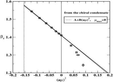
Figure 3: Critical couplings obtained from the chiral susceptibility, together with a linear fit in $(a\mu)^{2}$ to data with $\mu^{2}\leq 0$. The datum at $\beta_{c}=1.30$ (diamond) is taken from Ref. cea .

The fit results are summarized in Table 2 (rows for which the last entry is $(a\mu_{\rm max})^{2}=0$). The fit parameters have a tiny dependence on the observable considered. Moreover, the extrapolation of the critical line at $(a\mu)^{2}=-(\pi/8)^{2}$, corresponding to the first RW transition, is in good agreement with an independent determination of the RW endpoint Cor07 . This is a clear indication that the critical line is a continuation of the high-temperature first order RW transition line at $(a\mu)^{2}=-(\pi/8)^{2}$.

The extrapolation of the critical line to $\mu^{2}>0$ can be compared with the direct determinations of $\beta_{c}$ at $(a\mu)^{2}=0.04$, 0.0625 and 0.09. As one can see from Figs. 3, 4 and 5, there is discrepancy between the extrapolated critical line and the direct determinations of $\beta_{c}(\mu^{2})$ for each of the observables considered. The discrepancy is more pronounced when the susceptibility of the chiral condensate is used. This result implies that either the critical line is not analytic on the whole interval of $\mu^{2}$ values considered or it is in fact analytic, but the interpolation at $\mu^{2}\leq 0$ is not accurate enough to correctly reproduce the behavior at $\mu^{2}>0$.

Figure 4: Same as in Fig. 3 for the critical values of $\beta$ obtained via the Polyakov loop susceptibility.

Table 2: Parameters of various fits of the critical couplings according to $\beta_{c}(\mu^{2})=A+B(a\mu)^{2}+C(a\mu)^{4}+D(a\mu)^{6}$ (polynomial) or $\beta_{c}(\mu^{2})=[A+B(a\mu)^{2}]/[1+C(a\mu)^{2}]$ (ratio). Blank columns stand for terms not included in the fit. The last column reports the largest value of $(a\mu)^{2}$ included in each fit.

observable	fit	$A$	$B$	$C$	$D$	$\chi^{2}$/d.o.f.	$(a\mu_{\rm max})^{2}$
$\langle\overline{\psi}\psi\rangle$	polynomial	$1.4091(10)$	$-1.095(15)$			0.27	0.00
$\langle L\rangle$	polynomial	$1.3990(22)$	$-1.121(35)$			0.28	0.00
$\langle P\rangle$	polynomial	$1.4092(17)$	$-1.072(24)$			0.38	0.00
$\langle\overline{\psi}\psi\rangle$	polynomial	$1.4096(13)$	$-1.055(60)$	$0.33(48)$		1.35	0.00
$\langle L\rangle$	polynomial	$1.3989(32)$	$-1.13(13)$	$-0.1(1.1)$		0.35	0.00
$\langle P\rangle$	polynomial	$1.4105(22)$	$-0.986(94)$	$0.69(73)$		0.26	0.00
$\langle\overline{\psi}\psi\rangle$	ratio	$1.4096(13)$	$-0.64(65)$	$0.30(42)$		0.22	0.00
$\langle L\rangle$	ratio	$1.3989(32)$	$-1.22(1.45)$	$-0.06(95)$		0.35	0.00
$\langle P\rangle$	ratio	$1.4105(22)$	$-0.12(97)$	$0.62(63)$		0.26	0.00
$\langle\overline{\psi}\psi\rangle$	polynomial	$1.4088(99)$	$-1.230(25)$	$-3.77(35)$	$-22.7(3.6)$	1.00	0.09
$\langle L\rangle$	polynomial	$1.3963(22)$	$-1.303(53)$	$-2.71(52)$	$-11.2(6.6)$	0.43	0.09
$\langle P\rangle$	polynomial	$1.4096(17)$	$-1.110(40)$	$-1.78(60)$	$-12.6(5.7)$	0.29	0.09
$\langle\overline{\psi}\psi\rangle$	ratio	$1.4062(87)$	$-3.79(24)$	$-1.75(17)$		5.04	0.09
$\langle L\rangle$	ratio	$1.3948(18)$	$-3.67(39)$	$-1.66(27)$		0.58	0.09
$\langle P\rangle$	ratio	$1.4075(14)$	$-2.07(44)$	$-0.64(30)$		0.90	0.09

In order to discriminate between these two possibilities, we have interpolated all the available determinations of $\beta_{c}(\mu^{2})$, i.e. data for both $\mu^{2}\leq 0$ and $\mu^{2}>0$, with a unique analytic function. We have found that a polynomial of third order in $\mu^{2}$ nicely fits all data for $\beta_{c}(\mu^{2})$ for each of the three “probe” observables – see Fig. 6 for the case of the chiral condensate and Table 2 for a summary of the fit parameters and of the $\chi^{2}$/d.o.f.’s (rows for which the last entry is $(a\mu_{\rm max})^{2}=0.09$).

What happened here is a sort of “conspiracy”: the $\mu^{4}$ and $\mu^{6}$ terms compensate each other at large negative values of $\mu^{2}$ so that the effective interpolating function of the data at $\mu^{2}\leq 0$ is a first order polynomial in $\mu^{2}$. For $\mu^{2}>0$, instead, the $\mu^{4}$ and $\mu^{6}$ terms work in the same direction and their contribution cannot be neglected.

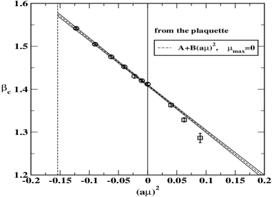
Figure 5: Same as in Fig. 3 for the critical values of $\beta$ obtained via the plaquette susceptibility.

For the cases of Polyakov look and plaquette, but not for the chiral condensate, we have obtained nice global interpolations also by means of a ratio of polynomials of the form $(A+B(a\mu)^{2})/(1+C(a\mu)^{2})$.

III Discussion and conclusions

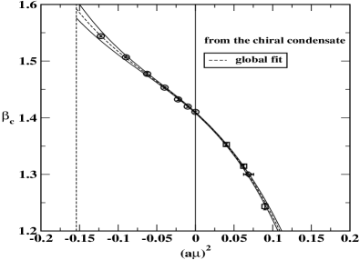
Figure 6: Same as in Fig. 3, but with the results of a fit to all data including terms up to $\mu^{6}$.

In this paper, we have tested in two-color QCD the analytic continuation of the critical line in the $T-\mu$ plane from imaginary to real chemical potential. We have found that the critical line around $\mu=0$ can be described by an analytic function. Indeed, a third order polynomial in $\mu^{2}$ nicely fits all the available data for the critical coupling. However, when trying to infer the behavior of the critical line at real $\mu$ from the extrapolation of its behavior at imaginary $\mu$, a very large precision would be needed to get the correct result. In the case of polynomial interpolations there is a clear indication that high-order terms play a relevant role at $\mu^{2}>0$ but are less visible at $\mu^{2}<0$, this calling for an accurate knowledge of the critical line in all the first RW sector. This scenario could be peculiar of two-color QCD. If confirmed in other theories free of the sign problem, such as QCD at finite isospin density, then one should seriously reconsider the analytic continuation of the critical line in the physically relevant case of QCD at finite baryon density. There the critical line at imaginary $\mu$ has been interpolated in most cases by a first order polynomial in $\mu^{2}$, the only exception being the use of Padé approximants in Ref. lom . If the scenario described in this paper, and in particular the “conspiracy” between the $\mu^{4}$ and $\mu^{6}$ terms, is robust, then it may be useful to revisit the interpolations used in QCD and to make the effort of determining accurately at least one more term in the polynomial fit.

References

- (1) I.M. Barbour et al., Nucl. Phys. Proc. Suppl. 60A, 220 (1998).
- (2) Z. Fodor, S.D. Katz, Phys. Lett. B 534, 87 (2002); JHEP 0203, 014 (2002).
- (3) Z. Fodor, S.D. Katz, C. Schmidt, JHEP 0703, 121 (2007)
- (4) Ph. de Forcrand and O. Philipsen, Nucl. Phys. B 642, 290 (2002); Nucl. Phys. B 673, 170 (2003).
- (5) M. D’Elia and M.P. Lombardo, Phys. Rev. D 67, 014505 (2003); Phys. Rev. D 70, 074509 (2004).
- (6) V. Azcoiti, G. Di Carlo, A. Galante and V. Laliena, Nucl. Phys. B 723, 77 (2005).
- (7) H.S. Chen, X.Q. Luo, Phys. Rev. D 72, 034504 (2005).
- (8) P. Giudice and A. Papa, Phys. Rev. D 69, 094509 (2004).
- (9) S. Kim, P. de Forcrand, S. Kratochvila, and T. Takaishi, PoS LAT2005, 166 (2006).
- (10) P. Cea, L. Cosmai, M. D’Elia and A. Papa, JHEP 0702, 066 (2007); PoS LAT2006, 143 (2006).
- (11) Ph. de Forcrand and O. Philipsen, JHEP 0701, 077 (2007); PoS LATTICE2007, 178 (2007).
- (12) M. D’Elia, F. Di Renzo, M.P. Lombardo, Phys. Rev. D 76, 114509 (2007).
- (13) S. Conradi, M. D’Elia, Phys. Rev. D 76, 074501 (2007).
- (14) P. Cea, L. Cosmai, M. D’Elia and A. Papa, PoS LATTICE 2007, 214 (2007).
- (15) F. Karbstein, M. Thies, Phys. Rev. D 75, 025003 (2007).
- (16) A. Roberge, N. Weiss, Nucl. Phys. B 275, 734 (1986).
- (17) S. Kratochvila, P. de Forcrand, PoS LAT2005, 167 (2006).
- (18) A. Alexandru, M. Faber, I. Horvath and K. F. Liu, Phys. Rev. D 72, 114513 (2005).
- (19) C.R. Allton et al., Phys. Rev. D 66, 074507 (2002); Phys. Rev. D 71, 054508 (2005).
- (20) R.V. Gavai and S. Gupta, Phys. Rev. D 68, 034506 (2003); Phys. Rev. D 73, 014004 (2006).
- (21) T.C. Blum, J.E. Hetrick and D. Toussaint, Phys. Rev. Lett. 76, 1019 (1996).
- (22) J. Engels, O. Kaczmarek, F. Karsch and E. Laermann, Nucl. Phys. B 558, 307 (1999).
- (23) R. De Pietri, A. Feo, E. Seiler and I.O. Stamatescu, Phys. Rev. D 76, 114501 (2007).
- (24) S.A. Gottlieb, W. Liu, D. Toussaint, R.L. Renken and R.L. Sugar, Phys. Rev. D 35, 2531 (1987).
- (25) G. Cortese, laurea’s thesis Università della Calabria.
- (26) M.P. Lombardo, PoS LAT2005, 168 (2006).