A Model-Independent Method of Determining Energy Scale and Muon Number in Cosmic Ray Surface Detectors

Abstract

Surface detector arrays are designed to measure the spectrum and composition of high-energy cosmic rays by detecting the secondary particle flux of the Extensive Air Showers (EAS) induced by the primary cosmic rays. Electromagnetic particles and muons constitute the dominant contribution to the ground detector signals. In this paper, we show that the ground signal deposit of an EAS can be described in terms of only very few parameters: the primary energy $E$, the zenith angle $\theta$, the distance of the shower maximum $X_{\rm max}$ to the ground, and a muon flux normalization $N_{\mu}$. This set of physical parameters is sufficient to predict the average particle fluxes at ground level to around 10% accuracy. We show that this is valid for hadronic air showers, using the two standard hadronic interaction models used in cosmic ray physics, QGSJetII and Sibyll, and for hadronic primaries from protons to iron. Based on this model, a new approach to calibrating the energy scale of ground array experiments is developed, which factors out the model dependence inherent in such calibrations up to now. Additionally, the method yields a measurement of the average number of muons in EAS. The measured distribution of $N_{\mu}$ of cosmic ray air showers can then be analysed, in conjunction with measurements of $X_{\rm max}$ from fluorescence detectors, to put constraints on the cosmic ray composition and hadronic interaction models.

, ,

1 Introduction

The origin of Ultra-High Energy Cosmic Rays (UHECR, with energies $E>10^{18}$ eV) still remains a mystery. Experimental results [1, 2, 3] suggest that the UHECR flux is composed predominantly of hadronic primary particles. As charged particles, they suffer deflections in cosmic magnetic fields and do not point back directly to their sources. Indirect proofs of their origin are necessary instead: the precise measurement of the energy spectrum, an estimation of the mass composition and its evolution with energy, and angular anisotropies are the three main handles on disentangling this almost century-old problem. Due to the interaction with the cosmic microwave background, UHECR suffer energy losses which limit their propagation distance [4, 5]. This “GZK horizon”, indications of which have already been observed in the UHECR spectrum [6, 7, 8], depends very sensitively on the energy and mass of the cosmic ray. In order to discern between different source scenarios, and to disentangle source characteristics from the effects of propagation, a precise knowledge of the energies of UHECR is crucial. Constraints on the composition of the cosmic ray flux at the highest energies will supply additional fundamental insight.

Due to the low fluxes at ultra-high energies, the detection of UHECR can only be achieved by measuring Extensive Air Showers (EAS), cascades of secondary particles resulting from the interaction of the primary cosmic rays with the Earth’s atmosphere. The measurement of the cosmic ray energy, flux, and mass composition relies on an understanding of this phenomenon.

Two main EAS detection techniques were developed over the years (see [9] for a review): surface detectors (SD) detect the particle flux of an EAS at a particular stage of the shower development; fluorescence detectors (FD) measure the shower development through nitrogen fluorescence emission induced by the electrons in the shower. The modeling of EAS through Monte Carlo simulations is needed in both fluorescence and surface detector experiments in order to interpret the data. We will show that hadronic EAS can be characterized, to a remarkable degree of precision, by only three parameters: the primary energy $E$, the depth of shower maximum $X_{\rm max}$, and an overall normalization of the muon component, which we call $N_{\mu}$. This is what we will call air shower universality [10]. The parameters $X_{\rm max}$ and $N_{\mu}$ are linked to the mass of the primary particle, ranging from proton to iron, and are subject to shower-to-shower fluctuations; proton showers have a larger depth of shower maximum than iron showers, while iron showers contain $\sim 40$% more muons than those induced by protons. Once measured, $N_{\mu}$ and $X_{\rm max}$ have to be compared with simulations to infer the cosmic ray composition and place constraints on hadronic interaction models. Previous studies have demonstrated that the energy spectra and angular distributions of electromagnetic particles [11, 12], as well as the lateral distribution of energy deposit close to the shower core [13] are all universal, i.e. they are functions of $E$, $X_{\rm max}$, and the atmospheric depth $X$ only. For studies of shower universality in the context of ground detectors, see [14, 15, 16]. EAS induced by photons show somewhat different properties, due to the absent hadronic cascade. Hence, it remains to be investigated to what extent the hadronic EAS universality studied here applies to photon showers.

By sampling the longitudinal development of the electromagnetic shower component close to the core, fluorescence detectors measure both $X_{\rm max}$ and $E$. The systematic uncertainty in the energy $E$ is typically 25%, mainly due to the uncertainties in the air fluorescence yield. A surface detector only samples the properties of an EAS at a given stage of the shower development and at several points at different distances $r$ from the shower axis. Rather than using the signal integrated over all distances, a quantity which shows large fluctuations, Hillas [17] proposed to use the signal at a given distance $r$ from the shower axis, $S(r)$, as a measure of the shower size, connected with the primary energy. The distance where experimental uncertainties in the size determination are minimized (the optimal distance $r_{\rm opt}$ [18]) is mainly determined by the experiment geometry, i.e. the spacing between surface detectors. $S(r_{\rm opt})$ is then related with the primary energy of the incoming cosmic ray using Monte Carlo simulations. This calibration has large systematics due to uncertainties in the hadronic models and the unknown primary cosmic ray composition.

In this paper, we will show how to use air shower universality to determine the calibration of a surface detector in a model-independent way. The signal $S(r_{\rm opt})$ is the sum of two components: an electromagnetic part which is well-understood and to a good approximation depends only on $E$ and $X_{\rm max}$ of the shower; and a muon part which, in addition to $E$ and $X_{\rm max}$, depends on the model and primary composition in terms of an overall normalization. The muon fraction can be determined by requiring that the shape of the zenith angle dependence of $S(r_{\rm opt})$ at a fixed energy, which depends on the muon normalization $N_{\mu}$, match the observed one. This method determines the energy scale of the experiment as well as the average number of muons produced in the air showers at a given energy.

Subsequently, we will apply air shower universality to data collected by a hybrid experiment, which combines the fluorescence technique with a surface detector. In this case, the calibration of the surface detector can be done almost independently of hadronic models and composition by using a small subset of the data (hybrid events) which are simultaneously measured by the fluorescence and the surface detector. Applying our method to hybrid data yields an event-by-event measurement of the muon content of the shower. This can be used as an independent cross-check of the measurement from the surface detector alone. Since the electromagnetic contribution to the signal varies with zenith angle, a hybrid measurement of $N_{\mu}$ at different zenith angles probes whether the electromagnetic part is described correctly by simulations, a key ingredient in our study. Conversely, the surface detector energy scale obtained with the universality-based method offers a cross-check of the hybrid calibration of the surface detector, which uses the fluorescence energy measurement.

In this work, we will not use data from any experiment, but we will use the Pierre Auger Observatory as a case of study. First results from this method applied to Auger data have already been presented in [19]. While we adopt the specifications of this experiment, the method presented here can be applied to any other surface detector (for example, AGASA [20]) or hybrid experiment (for example, Telescope Array [21]). The paper is organized as follows: in Sec. 2 we explain air shower universality, verifying it with the two standard high energy hadronic models used in cosmic ray physics (QGSJetII and Sibyll); in Sec. 3 the limits of air shower universality are shown; Sec. 4 presents the method of obtaining $N_{\mu}$ from the surface detector and determining the surface detector energy scale; in Sec. 5 we validate the method using a simple Monte Carlo approach; Sec. 6 shows how the approach can be applied to hybrid events; finally, the application to other experiments is discussed in Sec. 7; we conclude in Sec. 8.

2 Extensive air shower universality at large core distances

The results presented in this paper were obtained from a library of simulated EAS. We used CORSIKA 6.500 [22] with hadronic interaction models QGSJetII [23, 24] and Fluka [25] (proton and iron primaries, energies $10^{17.8}-10^{20}$ eV), and Sibyll [26, 27] / Fluka as well as QGSJetII / Gheisha [28] (proton at $10^{19}$ eV). For each primary/energy combination, we simulated 80 showers each at 7 zenith angles ranging from $0^{\circ}$ to 60^∘. Statistical thinning was employed in the simulations as describeds in [29], at a thinning threshold of $\varepsilon=10^{-6}$.

Using lookup tables generated with GEANT4 simulations [30], we calculated the average response of a cylindrical water Cherenkov detector (height 1.2m, cross section 10 m², similar to the type used in the Pierre Auger observatory) to each shower particle hitting the ground. See Sec. 7 for a discussion of the applicability to other experiments. The signals were calculated in two different approaches: 1.) Ground plane signals: The response is calculated for a realistic water tank on the ground. 2.) Shower plane signals: The response is calculated for a fiducial flat detector (with the same average particle response as the water tank) placed in the plane orthogonal to the shower axis (shower plane). Signals calculated in the shower plane procedure are not affected by detector geometrical effects, and therefore independent of the zenith angle. For details on the signal calculation, see appendix A. The shower plane signals will be useful to verify air shower universality, while the ground plane signals will be needed for the application to a realistic experiment (in our case the Pierre Auger Observatory).

Due to the statistical thinning procedure employed in the shower simulation, particles were collected in a sampling area of width 0.1 in $\log_{10}\>r$ centered around the shower core distance $r$ considered. This ensures, for a wide range of slopes of the lateral distribution, that the median radius of the energy deposit in the sampling area is indeed $r$. Signals are calculated in 18 azimuthal sectors, and normalized relative to the signal deposited by a vertically incident muon (VEM), a standard practice in surface detectors using the water Cherenkov technique.

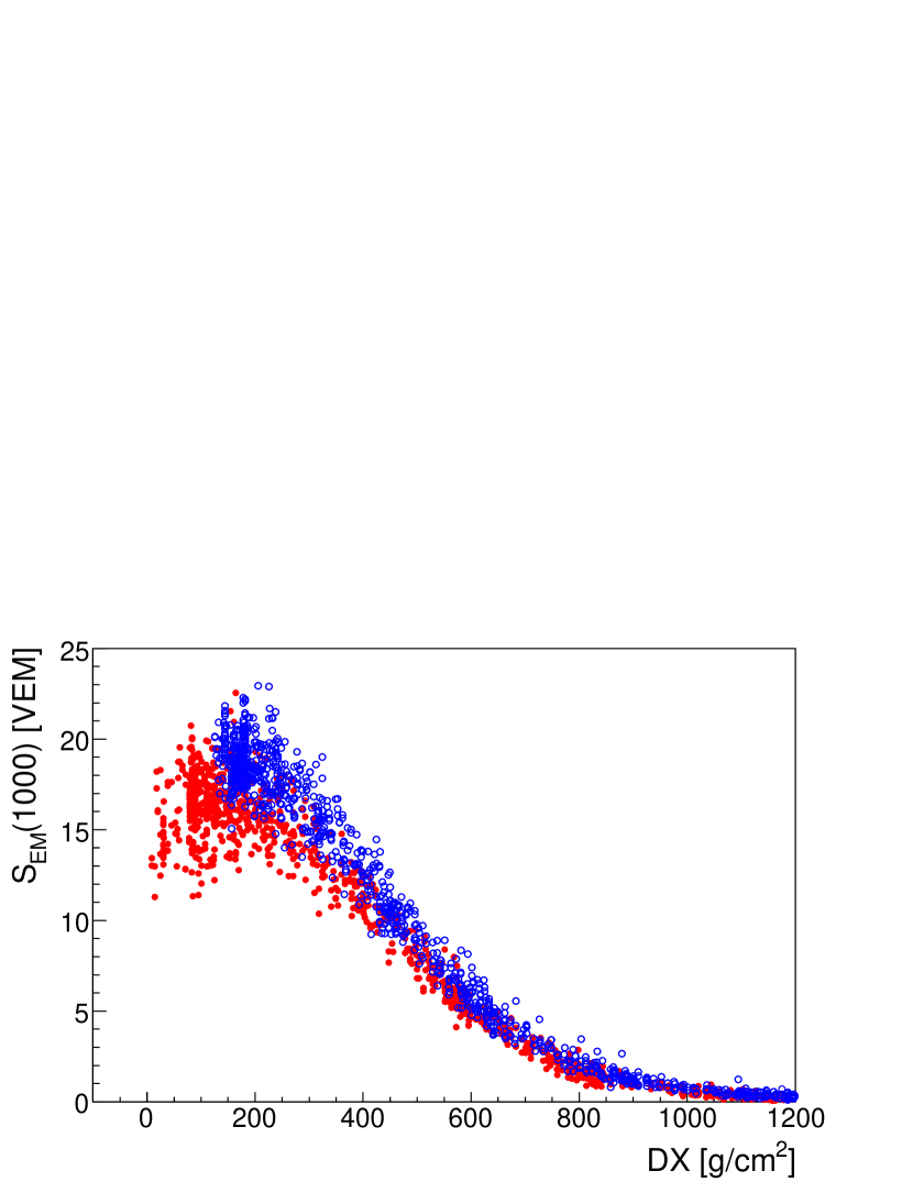
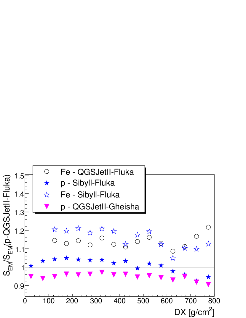
Figure 1: Left panel: Simulated electromagnetic shower plane signals at $r=1000$ m for proton (red dots) and iron showers (blue circles) at $10^{19}$ eV as a function of $DX$. The showers are simulated with QGSJetII/Fluka at discrete zenith angles spanning 0^∘ to $60^{\circ}$. Right panel: Simulated electromagnetic shower plane signals vs. $DX$ for different primaries and hadronic models, relative to the prediction for proton showers when using QGSJetII/Fluka.

To describe the stage of the shower development, we use the variable $DX$, defined as the distance from the detector to the shower maximum measured along the shower axis (in $\mbox{g}/\mbox{cm}^{2}$). For a tank on ground at a distance $r$ from the shower axis, $DX$ is:

$$DX=X_{\rm gr}\>\sec\theta-X_{\rm max}-r\>\cos\zeta\>\tan\theta\>\rho_{\rm air}$$ (1)

where $X_{\rm gr}$ is the vertical depth of the atmosphere, $\theta$ is the zenith angle, $X_{\rm max}$ is the slant depth of shower maximum, and $\zeta$ is the azimuthal angle in the shower plane such that $\zeta=0$ corresponds to a tank below the shower axis. $\rho_{\rm air}\approx 10^{-3}\mbox{g}/\rm cm^{3}$ is the density of air at ground level (see also Fig. 12 in the appendix). Often, we will consider signals averaged over azimuth. In this case, $DX$ is simply given by:

$$DX=X_{\rm gr}\>\sec\theta-X_{\rm max}$$ (2)

2.1 Electromagnetic and muon shower plane signals

At large core distances ($r\gtrsim 100$ m), the particle flux of EAS at ground is dominated by electromagnetic particles ($e^{+}$, $e^{-}$, $\gamma$) and muons. Throughout the paper, we include the signal from the electromagnetic products of in-flight muon decay in the muon contribution, separating it from the ‘pure’ electromagnetic part.

Fig. 1 (left panel) shows the electromagnetic shower plane signals $S_{\rm EM}$ of simulated proton and iron showers at $10^{19}$ eV as a function of $DX$ (in $\mbox{g}/\mbox{cm}^{2}$) for a core distance of 1000 m. For each tank, we calculate the corresponding $DX$ via Eq. (1) using the azimuth angle of the tank. Since zenith angle dependent detector geometry effects are removed in the shower plane treatment, we are able to compare the signals from a wide range of zenith angles. The electromagnetic signal shows a strong evolution with $DX$, reaching a maximum at $DX_{\rm peak}$ and rapidly attenuated for larger $DX$. $DX_{\rm peak}$ depends on core distance, being $0\>\mbox{g}/\mbox{cm}^{2}$ very close to the core and $\approx 200\>\mbox{g}/\mbox{cm}^{2}$ at 1000 m. This shift is only mildly dependent on $r$ in the range $400-1600$ m and it can be naturally explained by diffusion of electromagnetic particles away from the shower axis. Note that the overall electromagnetic signal as well as its evolution are slightly different for protons and iron. This is apparent in the right panel of Fig. 1, where the ratio of the signals obtained from different primary/model combinations to proton-QGSJetII is shown as a function of $DX$. The differences between models are around 5–10%, smaller than the deviation between proton and iron. This result is an extension to large $r$ of previous results [13, 12, 31] on the universality of the electromagnetic EAS component at small core distances. We address the difference ($\sim$ 15%) in $S_{\rm EM}$ between protons and iron in Sec. 3.

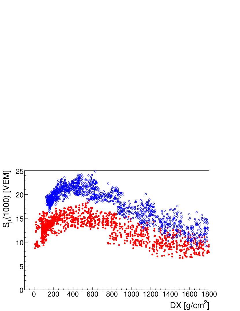
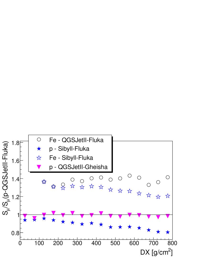
Figure 2: Left panel: Simulated muon signals $S_{\mu}$ at $r=1000$ m vs. $DX$ for the same $10^{19}$ eV proton (red dots) and iron showers (blue circles) as in Fig. 1. Note that $S_{\mu}$ includes the contribution from muon decay products. Right panel: Simulated muon signals vs. $DX$ for different primaries and hadronic models relative to the muon signal predicted for proton showers when using QGSJetII/Fluka. Note the difference in scale compared to Fig. 1.

Fig. 2 (right panel) shows the evolution of the muon signal $S_{\mu}$ with $DX$ (again for proton and iron showers at $E=10^{19}$ eV and $r$=1000 m). $S_{\mu}$ shows a distinctly different behavior: it peaks at $DX_{\rm peak}\approx 400\>\mbox{g}/\mbox{cm}^{2}$, and it is attenuated much more slowly than $S_{\rm EM}$. As expected, there is a dependence of the absolute normalization of the signals on the primary particle and hadronic model, which is clearly seen in Fig. 2 (right panel) where we again show $S_{\mu}$ obtained for different primaries and models relative to that of proton-QGSJetII. As for $S_{\rm EM}$, only differences in normalization and not in shape are apparent. We verified that the primary- and model-independence of the electromagnetic and muon signal evolution holds for shower core distances between 100 m and 1000 m.

2.2 Ground signal parameterization

In the previous section, we have shown that the evolution of the shower plane signals at a given shower core distance is only very weakly dependent on the primary particle or hadronic model considered. Therefore, a simple parameterization of the signals is possible. In this work, since we use the Pierre Auger Observatory as a case of study, we perform such a parameterization for $r$=1000 m. It has been shown [32] that the main observable in the surface detector of the Pierre Auger Observatory, $S(1000)$, is indeed a good measurement of the azimuth-averaged signal of particles at a core distance of $r=1000$ m. Hence, we separately parameterize the azimuth-averaged ground plane electromagnetic and muon signal at $10^{19}$ eV ($S_{\rm EM}(1000)$ and $S_{\mu}(1000)$, the total predicted signal being the sum of both), using the incomplete gamma, or Gaisser-Hillas-type function:

$$S(1000,\>DX)=S_{\rm max}\left(\frac{DX-X_{0}}{DX_{\rm peak}-X_{0}}\right)^{\alpha}\exp\left(\frac{DX_{\rm peak}-DX}{\lambda}\right),\;\;\alpha\equiv\frac{DX_{\rm peak}-X_{0}}{\lambda}\;$$ (3)

The four free parameters of this function are: $S_{\rm max}$ (the peak signal at 1000 m); $DX_{\rm peak}$(the slant depth relative to the overall shower maximum where the peak signal is reached); $\lambda$ (the attenuation length after the maximum); and $X_{0}$ (an additional shape parameter).

Fig. 4 shows the results of the fit for the muon signal. We have simultaneously fitted the predictions for different primaries (proton, iron) and different models (QGSJetII, Sibyll), keeping a separate normalization ($S_{\rm max}$) for each, while $\lambda$ and $DX_{\rm peak}$ are common to all. $X_{0}$ is not fitted but fixed to $-200\>\mbox{g}/\mbox{cm}^{2}$. The resulting parameters are summarized in Table 1, with $S_{\rm max}$ given for proton-QGSJetII. For the other model/primary combinations, we define a relative muon normalization given by $N_{\mu}=S_{\rm max}/S_{\rm max;ref}$, where we take proton-QGSJetII as the reference $S_{\rm max;ref}$. The $N_{\mu}$ for different models and primaries are listed in Table 2.

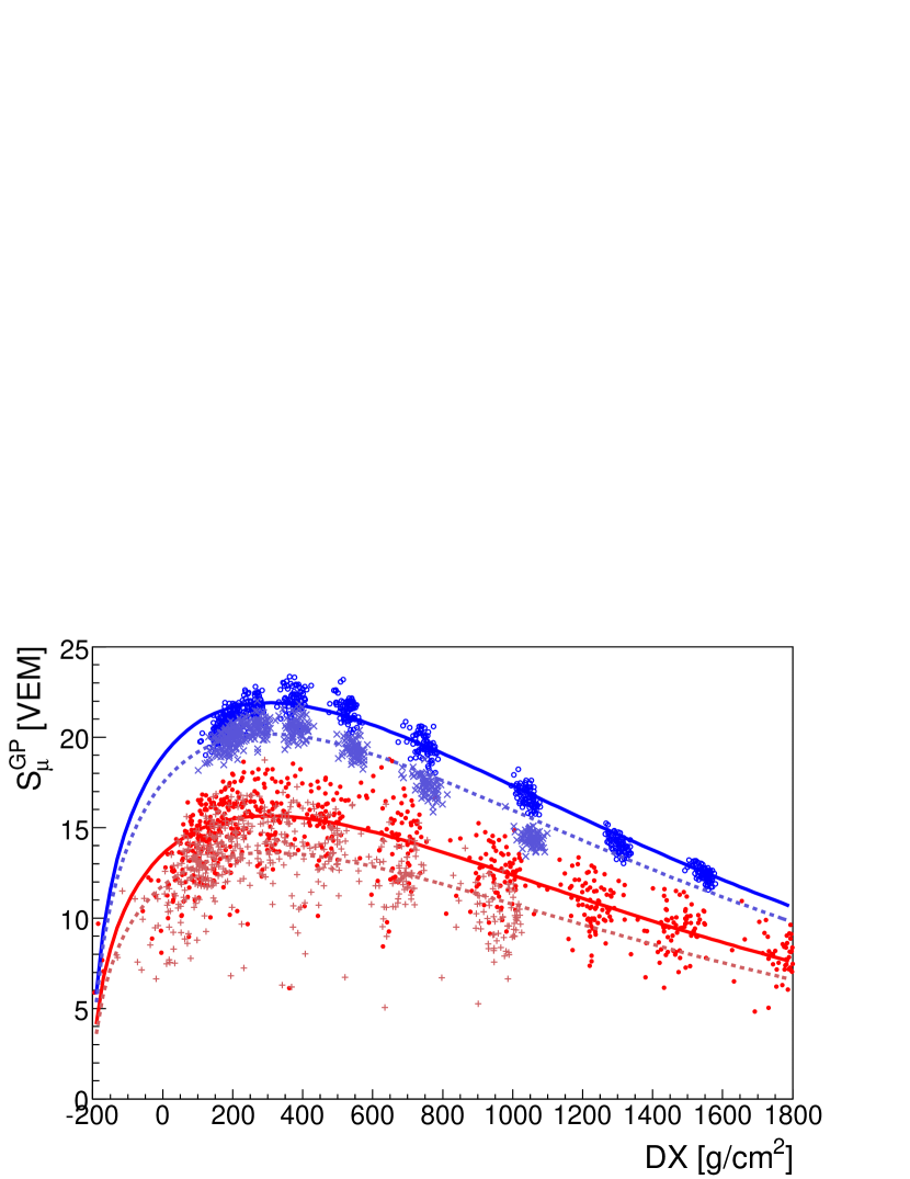
Figure 3: Parameterization of the muon ground plane signal ($E=10^{19}$ eV) at $r=1000$ m using Gaisser-Hillas functions (Eq. (3)). Red dots (crosses) denote proton-QGSJetII (proton-Sibyll) showers, blue circles (asterisks) are iron-QGSJetII (iron-Sibyll). The normalization is left free for each model/primary combination, while the other parameters are common to all.

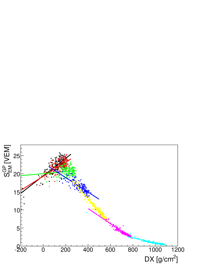
Figure 4: Electromagnetic ground plane signals (proton$-$dots; iron$-$crosses; QGSJetII) in zenith angle bands (color-coded). Proton and iron signals have been scaled symmetrically. A linear function is fit to the signal separately for each zenith angle band.

In the case of the electromagnetic signal, we have to take into account the detector geometrical effects, which cause differences in the signals from showers at two different zenith angles with the same $DX$ (see appendix A). Hence, we have to find a parameterization for $S_{\rm EM}(DX,\>\theta)$. The first step is to parameterize, for each of the 7 simulated zenith angles, the dependence of $S_{\rm EM}$ on $DX$; a linear function is found to be sufficient due to the limited $DX$ range at a fixed $\theta$. We scaled the proton and iron signals by $1+\alpha$ and $1-\alpha$, respectively (with $\alpha\lesssim 0.06$), to account for the deviations from universality. The deviations in the ground plane signals are slightly smaller than those shown in the previous section for the shower plane signals. Fig. 4 shows the results of the fits together with the direct Monte Carlo results, for the 7 fixed values of zenith angle.

In the second step, we fit a Gaisser-Hillas-type function (of $DX$) to $S_{\rm EM}(DX,\theta)$ for each $X_{\rm max}$ considered. The Gaisser-Hillas function is fitted to 7 equal-weight data points “predicted” from the 7 linear fits of the first step. This is equivalent to a parameterization of the dependence of $S_{\rm EM}$ on $\theta$ at a fixed $X_{\rm max}$, using an intermediate variable $DX(X_{\rm max},\theta)$. Table 1 gives the results for $X_{\rm max}=750\>\mbox{g}/\mbox{cm}^{2}$ and $X_{\rm gr}=875\>\mbox{g}/\mbox{cm}^{2}$. The second step may be applied to any value of $X_{\rm max}$, yielding a continuous function $S_{\rm EM}(\theta,DX(X_{\rm max},\theta))$ which depends on $\theta$ both explicitly and implicitly via $DX$. By contrast, since muons deposit a signal which is proportional to their pathlength in the water tank, the tank acts as a volume detector: the smaller projected area at higher zenith angle is canceled by the longer average tracklength. Hence, the average muon signal $S_{\mu}(DX)$ does not show an explicit $\theta$ dependence.

		$S_{\rm max}$	$DX_{\rm peak}$	$X_{0}$	$\lambda$
$S_{\rm EM}(1000)$	($X_{\rm max}=750\>\mbox{g}/\mbox{cm}^{2}$)	22.5	103.0	-540.6	102.7
$S_{\mu}(1000)$		15.6	302.4	-200	1109

Table 1: Fit parameters of the Gaisser-Hillas parameterization (Eq. (3)) of the universal electromagnetic and muon signal at $10^{19}$ eV. The electromagnetic parameterization is for a fixed $X_{\rm max}$ and $X_{\rm gr}=875\>\mbox{g}/\mbox{cm}^{2}$. For $S_{\mu\>\rm max}$, the value of proton-QGSJetII is given (for the other primaries and models relative to proton-QGSJetII, see Table 2).

At a fixed energy (here, 10 EeV), the parameterization presented above determines the average ground signal of a shower (at $r=1000$ m, azimuth-averaged):

$$S(1000)=S_{\rm EM}(\theta,\>DX(X_{\rm max},\theta))+N_{\mu}\cdot S_{\mu;\rm ref}(DX(X_{\rm max},\theta))$$ (4)

Here, $S_{\rm EM}$ denotes the parameterized electromagnetic signal, and $S_{\mu;\rm ref}$ is the reference muon signal which we take to be proton-QGSJetII. Hence, there are only three free parameters describing the average shower at this energy: the zenith angle $\theta$; the depth of shower maximum $X_{\rm max}$; and the normalization of the muon signal $N_{\mu}$ (relative to proton-QGSJetII).

We used the library of proton and iron showers with energies of $10^{18}-10^{20}$ eV to investigate the energy dependence of the evolution of $S_{\rm EM}$ and $S_{\mu}$ with $DX$. The electromagnetic signal normalization shows an energy scaling of $S_{\rm max;EM}\propto E^{0.97}$ (see also Sec. 3), while for the muon signal $S_{\rm max;\mu}\propto E^{\alpha}$ with $\alpha=0.9\dots 0.95$, depending on the hadronic model. All other fit parameters in Eq. (3) are independent of the primary energy in this energy range, for both $S_{\rm EM}$ and $S_{\mu}$, to within 5%.

Hence, Eq. (4) can be straightforwardly extended to other energies:

$$S(1000,E) = S_{\rm EM}(10\>\mbox{EeV},\theta,\>DX(X_{\rm max},\theta))\>\left(\frac{E}{10\>\mbox{EeV}}\right)^{0.97}$$ (5)

$$+ N_{\mu}(E)\cdot S_{\mu;\rm ref}(10\>\mbox{EeV},DX(X_{\rm max},\theta))$$

As the energy scaling of $S_{\mu}$ is slightly model-dependent, we treat it as an unknown and define $N_{\mu}(E)$ as the muon normalization at the energy $E$ with respect to the proton-QGSJetII reference at the fixed energy of 10 EeV.

2.3 Shower fluctuations

In addition to the overall behavior of the signals with $DX$ parameterized before, both electromagnetic and muon signals show fluctuations around the mean value. Fig. 5 shows the relative deviations of the ground plane $S_{\rm EM}$ (left panel) and $S_{\mu}$ (right panel) from the parameterization for proton and iron showers ($10^{19}$ eV, QGSJetII). These distributions contain showers from all zenith angles; no dependence of the relative fluctuations on zenith angle has been found. Note that the proton and iron electromagnetic signals are slightly shifted from 0 due to the universality violation (Fig. 1), whereas the deviations are centered around 0 for the muon signals (we used the corresponding muon signal normalizations for proton/iron).

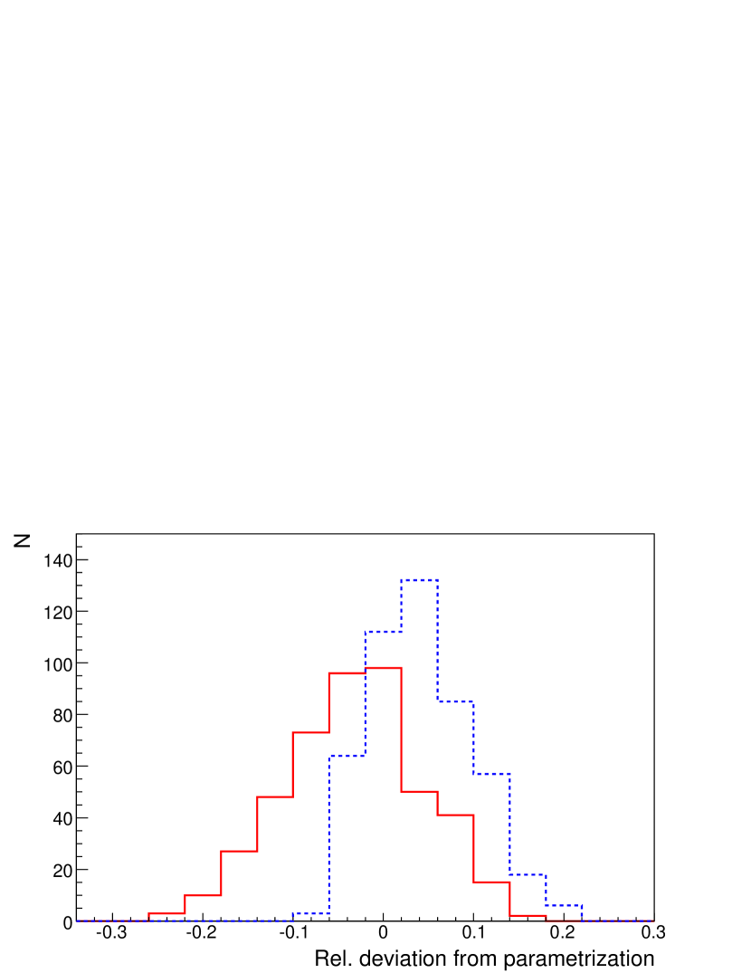
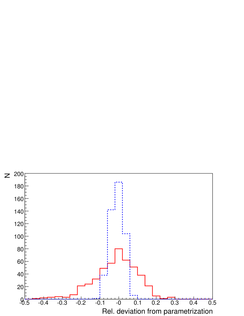
Figure 5: Left panel: Distribution of the relative deviations of the electromagnetic ground plane signals of showers at $10^{19}$ eV (QGSJetII) from the parameterization (Sec. 2.2). The red (solid) line is for proton, while the blue (dashed) is for iron. Right panel: The same for the muon ground plane signals.

The spread of the distribution shown in Fig. 1 and Fig. 2 has a contribution from the artificial fluctuations due to the thinning procedure used in the simulations. The fluctuations due to thinning can be estimated from vertical showers: since we expect the same signal in all azimuth sectors, thinning fluctuations are expected to be the dominant source of the variance between sectors. We find $\sigma_{\rm thin}=6.5$% for $S_{\rm EM}$ and 4% for $S_{\mu}$. We can then subtract the uncorrelated thinning variance from the total signal fluctuations to obtain the shower-to-shower fluctuations. Note that since we compare shower signals with the parameterization of the average signal at the same distance to ground $DX$, the signal fluctuations shown here are not caused by the fluctuations in the depth of shower maximum. The latter ones will induce additional fluctuations (mainly in the electromagnetic signal) that can be straightforwardly calculated convolving the fluctuations in $X_{\rm max}$ with the signal parameterization.

	RMS($S_{\rm EM}$)$/S_{\rm EM}$	RMS($S_{\mu}$)$/S_{\mu}$	$\langle X_{\rm max}\rangle$ (10 EeV)	$\tau_{X}$	$N_{\mu}$
Proton
QGSJetII	7.9%	11.8%	787.8$\>\mbox{g}/\mbox{cm}^{2}$	25.4$\>\mbox{g}/\mbox{cm}^{2}$	1
Sibyll	8.9%	12.4%	795.8$\>\mbox{g}/\mbox{cm}^{2}$	24.1$\>\mbox{g}/\mbox{cm}^{2}$	0.87
Iron
QGSJetII	5.4%	3.5%	708.7$\>\mbox{g}/\mbox{cm}^{2}$	10.9$\>\mbox{g}/\mbox{cm}^{2}$	1.40
Sibyll	4.8%	4.0%	696.5$\>\mbox{g}/\mbox{cm}^{2}$	10.2$\>\mbox{g}/\mbox{cm}^{2}$	1.27

Table 2: Relative shower-to-shower fluctuations of the electromagnetic and muon signals and parameters of the $X_{\rm max}$ distribution derived from QGSJetII and Sibyll showers at $10^{19}$ eV. The muon signal normalization $N_{\mu}$ relative to proton-QGSJetII for the different models is also shown. Note the differences in the absolute value of $\langle X_{\rm max}\rangle$ and $N_{\mu}$, while the fluctuations are model-independent.

We also parameterized the distribution of $X_{\rm max}$ for different primaries and models, using the following functional form:

$$\frac{dN}{dX_{\rm max}}\propto x^{4}\>e^{-x},\;\;0<x<\infty;\quad x=\frac{X_{\rm max}-\langle X_{\rm max}\rangle}{\tau_{X}}+5,$$ (6)

where $\langle X_{\rm max}\rangle$ denotes the mean depth of shower maximum, and $\tau_{X}$ is related to the RMS of the distribution via $\tau_{X}=\mbox{RMS}(X_{\rm max})/\sqrt{5}$. This asymmetric distribution is found to be a good fit to the $X_{\rm max}$ distributions for different primaries and models.

Table 2 summarizes the magnitude of fluctuations in $S_{\rm EM}$ and $S_{\mu}$ as well as $\tau_{X}$ for protons and iron using different hadronic models. Clearly, the shower-to-shower fluctuations in signal as well as $X_{\rm max}$ are independent of the hadronic model considered, but depend quite strongly on the primary particle. Hence, if measured, fluctuations can serve as a robust, model-independent indicator of composition. Our simulations predict that these fluctuations depend only very weakly on energy.

3 Limits of universality

The main discernible deviation from the universality approach adopted here is the difference in electromagnetic signal between proton and iron showers. This difference, which we refer to as universality violation, is larger than the differences found in the overall energy deposit in the atmosphere for proton and iron showers (for which in fact one finds the opposite effect: the so-called missing energy is larger for iron showers, [33]). Since we include muon decay products in the muon signal, this deviation is unrelated to the differences in muon content between protons and iron.

Fig. 7 shows the ratio of the number flux of electromagnetic particles for different combinations of primaries/models to the reference (proton/QGSJetII) as a function of $DX$ (again $r$=1000 m and $E=10^{19}$ eV). The differences between protons and iron is much smaller than in the case of the signals (Fig. 1), pointing to a slightly harder energy spectrum for electromagnetic particles at large $r$ in iron showers compared to proton showers. We also found that the discrepancy becomes smaller at smaller core distances. We have verified that the differences are independent of the details of nuclear fragmentation of the primary iron nuclei. This means that the nuclear binding of the 56 nucleons is not important for the EAS development. In other words, the superposition model holds, i.e., an iron shower can be considered as a superposition of 56 proton showers at $1/56$th of the primary energy.

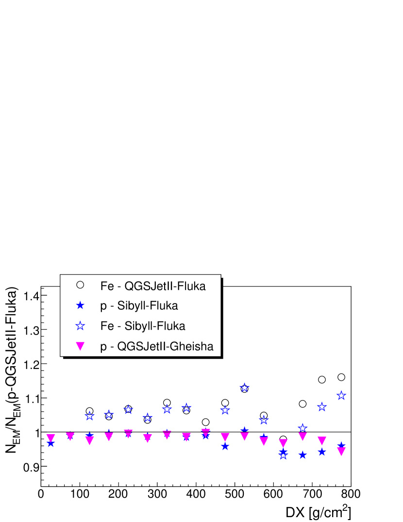
Figure 6: Number flux of electromagnetic particles in the shower plane at $r=1000$ m for different primaries and hadronic models at $10^{19}$ eV, relative to that of proton-QGSJetII.

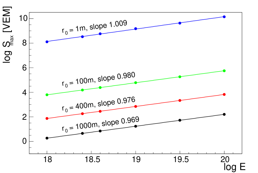
Figure 7: The parameter $S_{\rm max}$ of the parameterization Eq. (3) of electromagnetic shower plane signals as a function of primary energy, for different core distances $r$. Power-law fits and the resulting exponents are indicated.

This implies that the universality violation is due to a violation of strict linear energy scaling of the electromagnetic signal in hadronic shower simulations: if the electromagnetic signal scales as $E^{\alpha}$, $\alpha<1$, then the signal of an iron shower will be a factor of $56^{1-\alpha}$ times larger than that of a proton shower at the same energy. In order to explain the observed difference of $\sim 15$% in the shower plane signals, we would infer $\alpha\sim 0.97$. We have parameterized the electromagnetic signals for different energies and indeed found that the amplitude $S_{\rm max}$ of the signal (Eq. (3)) scales as $E^{0.97}$ at $r=1000$ m, with $\alpha$ approaching 1 as $r\rightarrow 0$ (Fig. 7). Note that, by parameterizing the complete evolution of the signal with $DX$, we take out the effects of the energy dependence of $X_{\rm max}$.

This violation of perfect energy scaling of the electromagnetic signal can be due to several reasons. The injection rate of energy into the electromagnetic part via $\pi^{0}$ decay as well as the energy spectrum of secondary $\pi^{0}$ might evolve with primary energy. In addition, the NKG theory of pure electromagnetic showers also predicts a slight deviation from perfect energy scaling of the particle flux on ground. These effects are currently under investigation.

4 Determining the muon normalization using the constant intensity method

One of the main challenges of a cosmic ray surface detector is to convert the ground signal $S(r)$ to a primary energy. As mentioned in Sec. 2.2, the universality-based signal parameterization has three free parameters. Apart from the zenith angle $\theta$ which is well measured along with the signal [32], the depth of shower maximum $X_{\rm max}$ and muon normalization $N_{\mu}$ (with respect to the reference signal at the fixed energy of 10 EeV) remain to be determined. Once these are known, Eq. (5) provides a one-to-one mapping of ground signal and energy, i.e. a model-independent energy scale of the experiment.

The mean depth $\langle X_{\rm max}\rangle$ of showers has been measured as a function of energy from experiments using the air fluorescence technique, e.g. HiRes [34] and Auger [35]. The knowledge of $\langle X_{\rm max}\rangle$ is important as it determines the average distance to shower maximum $DX$ for a given zenith angle, and the electromagnetic signal evolves strongly with $DX$. The overall precision of these $\langle X_{\rm max}\rangle$ measurements is better than $20\>\mbox{g}/\mbox{cm}^{2}$, and this small uncertainty in $\langle X_{\rm max}\rangle$ has only a limited effect on the estimated electromagnetic signal. Fig. 9 shows the limited effect of varying $X_{\rm max}$ by $\pm 14\>\mbox{g}/\mbox{cm}^{2}$ (the current measurement uncertainty at 10 EeV reported by Auger [35]) on $S_{\rm EM}$ as a function of $\sec\theta$.

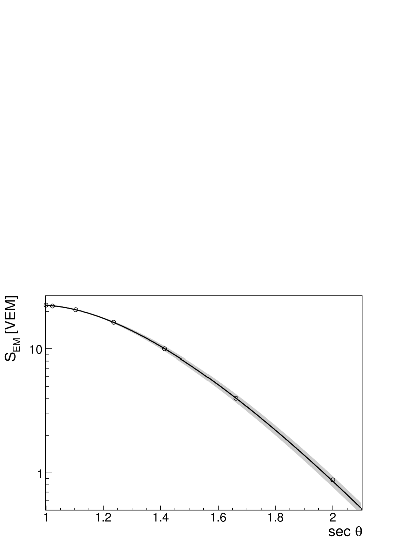
Figure 8: Parameterized electromagnetic signal at $10^{19}$ eV vs. $\sec\theta$ with $X_{\rm max}=750\>\mbox{g}/\mbox{cm}^{2}$ (black line, the dots indicate the signal parameterized at each zenith angle). The shaded band shows the effect on $S_{\rm EM}$ of a variation of $X_{\rm max}$ by $\pm 14\>\mbox{g}/\mbox{cm}^{2}$.

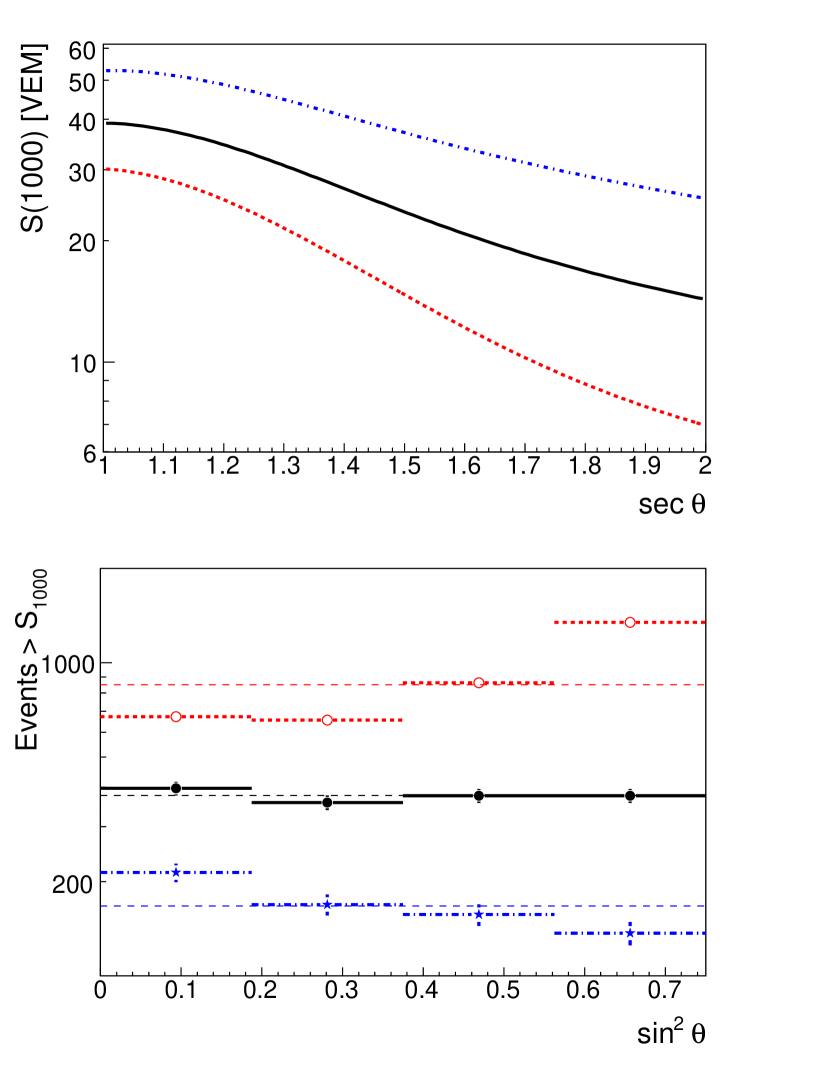
Figure 9: Upper panel: the signal parameterization at 10 EeV Eq. (4) vs. $\sec\>\theta$ for different $N_{\mu}$ (black/solid$-$1.1, red/dashed$-$0.5, blue/dash-dotted$-$2.0). Lower panel: histograms of number of events above the parameterized signal in equal exposure bins, obtained from a Monte Carlo data set with a true $N_{\mu}$ of 1, for the different $N_{\mu}$ values shown in the upper panel.

The main uncertainty in determining the energy scale of surface detectors is thus in the value of $N_{\mu}$. Fortunately, one can make use of the different behavior of $S_{\rm EM}$ and $S_{\mu}$ with $DX$ (and hence, $\sec\theta$) to measure $N_{\mu}$ via the constant intensity method (Fig. 9): dividing the data set into equal exposure bins in zenith angle, i.e., bins of $\sin^{2}\theta$, a correct signal-to-energy convertor should yield the same number of events in each bin with measured signal greater than the parameterized signal at a fixed energy. This is due to the isotropy ($\theta$-independence) of the cosmic ray flux, which requires that the number of events $N(>E)$ above a fixed energy $E$ should be equal in equal exposure bins.

Fig. 9 (upper panel) shows the zenith angle dependence of the signal (Eq. (4)) for a fixed energy of 10¹⁹ eV and different values of $N_{\mu}$. Apart from the overall change in signal, it is evident that the smaller the $N_{\mu}$, the steeper the $\theta$ dependence is. We now divide a simulated ground detector data set with a “true” $N_{\mu}(10^{19}\rm eV)=1$ (see Sec. 5 for details on the simulation) in equal exposure bins in zenith angle. Given a muon normalization, we calculate the number of events in each bin that are above a given reference energy (here $E_{\rm ref}$=10¹⁹ eV), according to Eq. (4) with the given $N_{\mu}$. We then adjust $N_{\mu}(E_{\rm ref})$ in the signal parameterization Eq. (4) to the value which gives an equal number of events $N(>S(E_{\rm ref},\theta))$ in each zenith angle bin (lower panel in Fig. 9). Clearly, a too low value of $N_{\mu}$ results in an excess of events at high $\theta$ (the parameterized signal has a too steep attenuation with $\sec\theta$), whereas a too high $N_{\mu}$ results in a deficit of high zenith angle events ($\sec\theta$ attenuation too shallow). In this calculation we used the $\langle X_{\rm max}\rangle$ at 10 EeV reported in [35] to calculate the ground plane signals. Note that an $N_{\mu}$ of 1.1 gives a flat distribution, whereas the “true” $N_{\mu}$ used is 1.0. This bias in the $N_{\mu}$ measurement will be addressed in the next section.

For a range of $N_{\mu}$ values, we then calculate the $\chi^{2}$/dof of the event histogram relative to a flat distribution in $\sin^{2}\theta$. Fitting a parabola to the function $\chi^{2}(N_{\mu})$ yields the best-fit $N_{\mu\>\rm fit}$ and its error $\sigma_{N_{\mu}}$:

$$\chi^{2}(N_{\mu})=\chi^{2}_{\rm min}+\left(\frac{N_{\mu}-N_{\mu\>\rm fit}}{\sigma_{N_{\mu}}}\right)^{2}$$ (7)

For a data set comparable to current Auger statistics ($\sim$11 000 events above 3 EeV [7]), we expect a statistical error of $\sigma_{N_{\mu}}=0.1$. Once $N_{\mu}$ is known, the knowledge of $S_{\rm EM}$ (within the uncertainty of $\sim\pm 6$% due to universality violation) determines a model-independent energy scale, with a statistical error of $\sigma_{N_{\mu}}\cdot S_{\mu;\rm ref}$ around 4%. The constant intensity method can be extended to other energies, using the energy-dependent parameterization Eq. (5) in Sec. 2.2. This yields a measurement of $N_{\mu}(E)$, comparable to the measurement of $\langle X_{\rm max}\rangle$ in its sensitivity to the primary composition. Table 3 contains a summary of the expected statistical and systematic errors from current and upcoming experiments.

In Fig. 10 we show possible results of this measurement, the integral measurement of $N_{\mu}(E)$ (solid black line, corrected for the bias, see Sec. 5) and with 1$\sigma$ statistical error band (shaded) after a three year Auger exposure. Here, we took $N_{\mu}(E)=1.2(E/10\>\mbox{EeV})^{0.85}$ as fiducial value. As the cosmic ray spectrum drops rapidly with energy ($\propto E^{-3}$), the average energy of cosmic rays above a given energy threshold is very close to that threshold. Hence, for slow changes of the cosmic ray composition with energy, the $N_{\mu}$ value determined from the constant intensity method will reflect the actual average value of $N_{\mu}$ for cosmic rays at that energy (this will be shown in the next section). In case of an abruptly changing composition, the measured $N_{\mu}(E)$ will clearly show evidence for this. However, the interpretation of the integral $N_{\mu}$ measurement in terms of composition will have to rely on a modeling of the composition evolution in this case. In addition, the measurement of $N_{\mu}(E)$ can place constraints on hadronic models, whose predictions are shown as lines in Fig. 10.

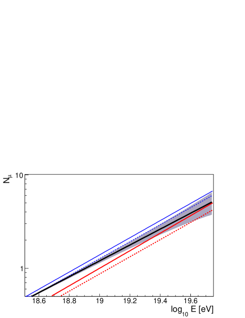
Figure 10: The measured muon normalization $N_{\mu}$ as a function of energy (thick black line) with statitistical error band expected from a three-year Auger exposure (shaded), for a fiducial $N_{\mu}(E)=1.2\>(E/10\>\mbox{EeV})^{0.85}$. Also shown are model predictions for iron (upper two lines, blue; solid$-$QGSJetII, dashed$-$Sibyll) and proton showers (lower two lines, red; solid$-$QGSJetII, dashed$-$Sibyll).

	Muon normalization $N_{\mu}$	Energy scale
Statistical error
current Auger	0.1	4%
Systematic errors
$\langle X_{\rm max}\rangle$ uncertainty (14$\>\mbox{g}/\mbox{cm}^{2}$ [35])	+0.05 / -0.07	+0.5% / -2%
Universality violation	+0.01 / -0.04	+3% / -4%
$N_{\mu}$ bias	$\lesssim$10%	$\lesssim 5$%

Table 3: Expected statistical (for current Auger exposure) and systematic errors on the muon normalization $N_{\mu}$ and energy scale $S(\theta=\theta_{0},\>E=10\>\rm EeV)$ at 10 EeV.

5 Validating the constant intensity method

To benchmark and validate the determination of $N_{\mu}$ via the constant intensity method, we simulate realistic data sets based on our parameterization of the ground signal (Sec. 2.2) and its fluctuations (Sec. 2.3). The fluctuations in signal as well as $X_{\rm max}$ could have an impact on the measurement of $N_{\mu}$, since only the average values are used to infer $N_{\mu}$ (Sec. 4). Additionally, a mixed composition of the cosmic ray beam could bias the measurements. The purpose of this section is to quantify systematic uncertainties of the method described before.

The calculation of a simulated data set proceeds as follows. Event energies are drawn from a spectrum $dN/dE\propto E^{-2.9}$ in the range $10^{17.8}-10^{20.2}$eV, while the zenith angle is drawn from an isotropic distribution ($\theta<70^{\circ}$). The primary particle type (proton or iron) is chosen at random according to a given mixture. The depth of shower maximum is then drawn from the distribution Eq. (6) with the parameters for the given primary (we adopt the parameters from QGSJetII; this has no influence on our conclusions). An $N_{\mu}$ is determined according to the primary. With $E$, $\theta$, $X_{\rm max}$, and $N_{\mu}$ given, the ground signal can be determined via Eq. (4) (we scale $S_{\rm EM}$ with $E^{0.97}$, and $S_{\mu}$ with $E^{0.9}$). The two signal components are fluctuated according to the primary (see Table 2). Finally, we cut events according to a simple trigger depending on the ground signal, and apply signal reconstruction uncertainties as reported by the Auger observatory [32]. The main characteristics of the reconstruction of $S(1000)$ are that it is unbiased at large signals $S(1000)\gtrsim 10$ VEM, and that bias and variance increase quickly for signals below 10 VEM.

A large set of simulated data sets showed that the error calculation according to Eq. (7) is a good estimator for the variance of the $N_{\mu}$ measurement. However, we found that the constant intensity method yields a systematic shift to higher $N_{\mu}$ values of about 5–10%. This can be explained by trigger effects and fluctuations. Due to the attenuation of the signal with zenith angle at a fixed energy, the resolution gets worse at large zenith angles. Additionally, upward fluctuations above the trigger threshold are more important at high zenith angles. These two effects, in the presence of a steep spectrum, produce a zenith angle-dependent enhancement of the number of events reconstructed above a given energy. This tends to flatten the constant intensity curve (Fig. 9), which leads to a higher estimated $N_{\mu}$ value. The bias in $N_{\mu}$ is mainly determined by the experimental resolution and trigger effects. It depends slightly on the primary composition, ranging from 4% for pure iron to 8% for a mixed composition, due to the differing magnitudes of shower-to-shower fluctuations. The unknown composition, and imperfect knowledge of the experimental characteristics, lead to an uncertainty in the bias which should be included in the systematic error on $N_{\mu}$. We assume that this error will be smaller than the absolute value of the bias, hence $\lesssim$10%.

Further systematics of $N_{\mu}$ are the violation of universality in the electromagnetic ground signal ($\sim\pm 6$%, Sec. 2.2), and the uncertainty in the value of $\langle X_{\rm max}\rangle$, which translates into a further uncertainty in the electromagnetic signal. Table 3 gives a summary of the systematic errors derived for $N_{\mu}$ and the energy scale (i.e., $S(\theta=\theta_{0},\>E=10\;\rm EeV)$, we take $\theta_{0}=38^{\circ}$, close to the median of the isotropic cosmic rays), all evaluated at 10 EeV. We stress that since the universality violation is smaller closer to the shower core, this method exhibits significantly smaller systematics when applied to a surface detector measuring the signal at $r=600$ m, instead of 1000 m as considered here.

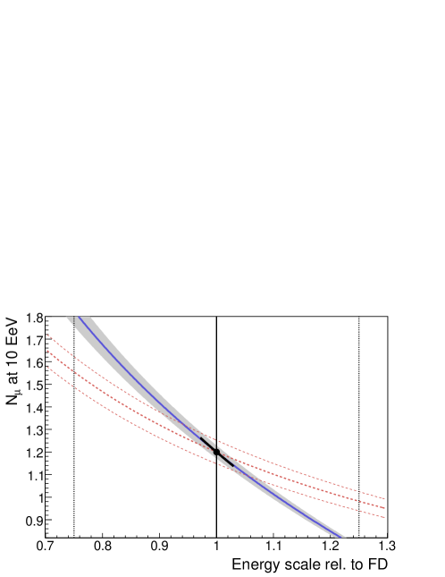
Figure 11: Constraints in the $N_{\mu}$-energy scale plane placed by three independent measurements: the constant intensity method (black dot with error); vertical hybrid events (blue solid line with shaded error band); inclined hybrid events (red dashed lines). An error of 25% in the fluorescence energy scale is indicated (vertical lines). All values are calculated for a three year Auger-equivalent exposure. The fiducial $N_{\mu}$ is 1.2.

6 Cross-checks and independent hybrid measurements

The constant intensity method described above is independent of the primary composition and hadronic interaction models (within systematics), and also independent from other energy calibrations (e.g., fluorescence telescopes). However, it relies on a good understanding of the electromagnetic part of air showers as well as detector bias and resolution (Sec. 5). Hence, it is desirable to cross-check the results of the method with independent data.

Hybrid experiments, which simultaneously measure the ground signal as well as fluorescence energy and $X_{\rm max}$ on an event-by-event basis, allow several cross-checks of the $N_{\mu}$ measurement. Due to the uncertainty in the energy scale of the fluorescence detector ($\sim$ 25%), we introduce a scaling factor ($f_{FD}$) of the measured fluorescence energy.

Using the parameterized electromagnetic signal $S_{\rm EM}(DX(\theta,X_{\rm max}),\theta,E)$ (Sec. 2.2), with $E=f_{FD}E_{FD}$ and $X_{\rm max}$ given by the fluorescence measurement, we can, for a single event, determine the muon signal $S_{\mu}$ at a fixed core distance by subtracting the electromagnetic component from the total signal (see Eq. (5)). The muon normalization is then given by $N_{\mu}=S_{\mu}/S_{\mu;\rm ref}$, where $S_{\mu;\rm ref}$ is the reference parameterized muon signal (proton-QGSJetII) at 10 EeV. Additionally, we can divide the hybrid data into two sets: vertical and inclined events, with zenith angles smaller and larger than 60^∘, respectively. In inclined events the electromagnetic signal at ground is essentially negligible, and the ground signal allows for a direct measurement of the muon signal. We can then calculate the mean measured $\langle N_{\mu}\rangle$ for vertical and inclined events as a function of $f_{FD}$. Fig. 11 shows the results for vertical (blue line with shaded error band) and inclined (red lines) events for an experiment with 3 years Auger-equivalent exposure. In order to measure $\langle N_{\mu}\rangle$ with hybrid events we clearly need to constrain $f_{FD}$. The black dot in Fig. 11 corresponds to the result of the constant intensity method described in the previous sections. It constrains $N_{\mu}$ as well as the energy scale. The fluorescence energy scale and its current uncertainty ($f_{FD}=1.0\pm 0.25$) are indicated in the graph by vertical lines.

The crossing point of the three $N_{\mu}$ measurements is an important cross-check of the universality-based method: only a correct description of the evolution of the electromagnetic and muon ground signals will lead to a unique crossing point. The value of $f_{FD}$ that corresponds to the crossing point is a quite powerful fluorescence-independent measurement of the energy scale. The statistical uncertainty of this measurement is much smaller than the current uncertainty on the fluorescence energy scale, and thus provides for a sensitive cross-check. At the same time, experimental efforts to reduce the systematic fluorescence energy uncertainty are in progress [36].

Hybrid events offer several further ways to place constraints on hadronic models. For example, since $S_{\mu}$ and $DX$ are measured independently for each hybrid event, the behavior of $S_{\mu}(DX)$ can be inferred, which contains information on the energy spectrum of muons in UHE air showers. In addition, the measured fluctuations of $N_{\mu}$ allow for model-independent constraints on the primary composition, if the reconstruction uncertainties are well understood. In addition, observed anomalous $N_{\mu}$ values in single events can be used to search for non-hadronic primaries. Photon showers have a muon component of about $1/10$th of a proton shower and thus could leave a distinctive signature in the observed $N_{\mu}$. However, the sensitivity of this method to photon showers remains to be studied quantitatively with simulations of photon showers.

7 Application to other experiments

The methodology and results presented so far have been specialized to the case of Auger. We now discuss the applicability to other current and future experiments. The main experiment characteristic determining this application is the ratio of the electromagnetic and muon contributions to the shower size observable ($S(1000)$ in the case of Auger).

If the muon contribution is very small, the signal becomes essentially independent of $N_{\mu}$, and only the knowledge of $\langle X_{\rm max}\rangle$ is needed to predict the average signal in a model-independent way. An experiment operating in this regime (such as AGASA [37]) is able to experimentally verify the electromagnetic signal predicted by simulations.

Conversely, if the muon contribution dominates even at small zenith angles, the attenuation (i.e., $\theta$-dependence) of the signal becomes very small, and a model-independent separation of the electromagnetic and muon components is impossible. The method of determining the energy scale using the constant intensity method is then not applicable. However, the attenuation curve can still be measured experimentally and compared with the prediction from simulations, which depends on the energy spectrum of muons produced in EAS. In addition, hybrid events with an independent energy measurement allow for a measurement of the absolute muon signal normalization with respect to simulations.

The ratio of muon to electromagnetic signal is determined by three factors in the experimental setup: 1.) The detector type: thin scintillator detectors have equal response to all minimum ionizing particles and thus operate as particle counters. The measured number flux of particles is dominated by electromagnetic particles. Shielding can however make scintillator detectors sensitive to muons as well. By contrast, muons deposit a large signal in water Cherenkov detectors. In this case, the ratio of area to height of the water volume determines the EM$/\mu$ ratio (flatter tanks yielding a larger ratio). 2.) The detector spacing: the spacing determines the distance at which the signal is measured [18]. Since the lateral distribution of the muon signal is more spread out than the electromagnetic signal, increasing the spacing will increase the relative muon contribution in the measured particle flux. 3.) The stage of shower evolution probed: this depends on the height above sea level of the experiment and the range of primary energy observed. Showers observed very far from the shower maximum have a small electromagnetic component.

Due to different characteristics, the ground signal will be dominated by the electromagnetic part in some experiments (e.g., AGASA, EASTop, Telescope Array), whereas the muon signal will contribute significantly at others (e.g., Auger, Haverah Park). A possible quantitative criterion for the applicability of the constant intensity method is the significance of the signal attenuation observed (e.g., $S(\theta=0^{\circ})/S(\theta=60^{\circ})$) with respect to the statistical and systematic errors in the signal determination. This criterion corresponds to an upper limit on the relative muon signal contribution, which has a very weak dependence on zenith angle.

8 Discussion and conclusion

We have shown how Monte Carlo predictions of ground signals can be used to determine the energy scale of surface detector experiments, indepedently of the cosmic ray composition and hadronic interaction models. This method overcomes the otherwise unavoidable systematics of surface detectors due to the unknown cosmic ray composition. In addition, it allows for a clean measurement of the number of muons in extensive air showers. In light of the recent detection of a possible GZK feature in the UHECR spectrum, the energy scale of cosmic ray experiments is of crucial importance to distinguish between different UHECR source scenarios. Hence, it is desirable to determine the energy scale with several methods. The measurement of the surface detector energy scale presented here is completely independent of the energy scale determined from fluorescence detectors, and contains different systematic uncertainties.

In this paper, we explored only a single surface detector observable, the signal $S(r)$ at a fixed distance from the shower axis. The methodology can be extended to parameterize the signal at different distances and azimuth angles. An extended parameterization like this can then be compared with each detector station in a given event, increasing the number of observables for each event. Ideally, perhaps in combination with other observables like the rise time [38, 39, 40], this could be used to break the degeneracy of $N_{\mu}$ and energy on an event-by-event basis for a surface detector alone.

It is important to note, however, that air shower universality, the basis of this methodology, can be violated by new mechanisms in hadronic interactions in EAS. Recently, the hadronic interaction model EPOS has been introduced [41, 42]. While the predictions for the depth of shower maximum are within the range of the previous models considered here, EPOS shows considerable deviations in the ground signal predictions: at 10¹⁹ eV, the EPOS electromagnetic signal seems to be $\sim 20$% larger than in the other models, while the predicted muon signal is 50–70% higher. These differences are due to the production of secondary baryon-antibaryon pairs in the GeV range which is strongly increased in EPOS. These baryons then produce more muons and a flatter lateral distribution of the signal compared to the other models. These predictions, while violating air shower universality, can be constrained by observations using the methodology presented here: by separately parametrizing the electromagnetic and muon signals predicted by EPOS, one can infer the relative muon normalization with respect to EPOS which is required by the data. We would like to point out that EPOS can be compared with cosmic ray data at lower energies (e.g. KASCADE [43]), as it was done in the past with the QGSJetII and Sibyll2.1 models. In addition, accelerator experiments [44] are underway to measure the baryon pair production at the relevant energies. One might hope that, once the magnitude of the baryon-antibaryon production is understood, hadronic models will converge to a universal prediction of the electromagnetic part as shown here for QGSJetII and Sibyll.

Very generally, the methodology presented here allows for a clean comparison of Monte Carlo simulations with air shower data, by separating shower evolution effects from primary composition and high-energy interactions. In applying air shower universality, current and future experiments have the potential to tightly constrain high energy hadronic models, as well as the energy scale and mass composition of the cosmic ray beam.

Appendix A Geometrical effects, ground plane and shower plane signals

Fig. 12 shows a sketch of an inclined shower hitting the ground. Two detectors at the same distance from the shower core correspond to different stages in the shower development, i.e. different $DX$ (Eq. (1)). The signal size in inclined showers shows a modulation with $\zeta$ angle. This modulation or signal asymmetry is produced by a convolution of effects [10]. The first one is due to the $\zeta$ dependence of $DX$ for inclined showers (Eq. (1)). In addition, there is a geometrical effect which depends on the detector geometry and zenith angle of the shower.

Consider the flux of shower particles $\mathbf{\Phi}$ at a given $DX$ and $r$, so that the number of particles entering the detector is $\mathbf{\Phi}\cdot\mathbf{A_{d}}$, where $\mathbf{A_{d}}$ is the vector associated with the detector surface with $|\mathbf{A_{d}}|$ equal to its area. $\mathbf{\Phi}$ is invariant under rotations around the shower axis, and it only depends on $r$ and $DX$. For vertical showers, the number of particles $\mathbf{\Phi}\cdot\mathbf{A_{d}}$ is invariant under rotations around the shower axis. For inclined showers, however, this is not the case, since $\mathbf{\Phi}$ is not parallel to the shower axis (Fig. 12). We therefore expect detectors at the same $r$ but different $\zeta$ angles to be hit by different numbers of particles, even if $\mathbf{\Phi}$ was independent of $DX$.

Hence, the ground-plane signals depend on $DX$, $r$ and $\theta$. To suppress the dependence on $\theta$ and decouple shower development effects from geometrical effects, we define the shower plane signal as the signal generated by shower particles passing through the top surface of a detector placed perpendicular to the shower axis. This allows us to combine different zenith and $\zeta$ angles when plotting the shower-plane signal vs $DX$ (e.g., Fig. 1).

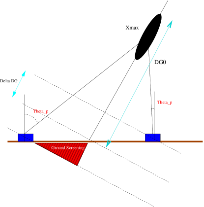
Figure 12: Sketch of an inclined shower hitting the ground level. The $DX$ of each tank is its distance to the shower maximum, projected on the shower axis ($DX_{0}$ $\pm$ $\Delta_{DX}$ in the sketch).

While the ground signals can be straightforwardly calculated from the simulation output particles (taking into account the statistical weight $W$ due to thinning), the shower plane signals are calculated in the following way.

Consider a particle with weight $W$ and unit momentum vector $\mathbf{\hat{p}}$ hitting a sampling region at ground. We will associate a flux $\mathbf{\Phi_{i}}$ to this particle in such a way that:

$$N^{GP}=W=\mathbf{\Phi_{i}}\cdot\mathbf{A_{s}^{GP}}=\Phi_{i}\>A_{s}^{GP}\>\mathbf{\hat{p}}\cdot\mathbf{\hat{g}}$$ (8)

where $N^{GP}$ is the number of particles hitting a ground sampling area $A_{s}^{GP}$ ($\sim 10^{5}\>\rm m^{2}$), and $\mathbf{\hat{g}}$ is the unit normal to the ground. Therefore, the flux associated with a particle of weight $W$ is given by:

$$\mathbf{\Phi_{i}}=\frac{W}{\mathbf{\hat{p}}\cdot\mathbf{\hat{g}}\>A_{s}^{GP}}\mathbf{\hat{p}}\\$$ (9)

The number of particles crossing the corresponding sampling area $A_{s}^{SP}$ in the shower plane is given by the scalar product of this flux and a vector parallel to the shower axis with a normalization equal to $A_{s}^{SP}$:

$$N_{i}^{SP}=\mathbf{\Phi_{i}}\cdot\mathbf{A_{s}^{SP}}=W\>\frac{\mathbf{\hat{p}}\cdot\mathbf{\hat{a}}}{\mathbf{\hat{p}}\cdot\mathbf{\hat{g}}}\frac{A_{s}^{SP}}{A_{s}^{GP}}=W\>\frac{\mathbf{\hat{p}}\cdot\mathbf{\hat{a}}}{\mathbf{\hat{p}}\cdot\mathbf{\hat{g}}}\mathbf{\hat{a}}\cdot\mathbf{\hat{g}}$$ (10)

where $\mathbf{\hat{a}}$ is a unit vector along the shower axis, and we used $A_{s}^{SP}/A_{s}^{GP}=\mathbf{\hat{a}}\cdot\mathbf{\hat{g}}$.

The shower-plane signal of a detector is then given by:

$$S^{SP}=\sum_{i}\>N_{i}^{SP}~{}\frac{A_{\rm tank}}{A_{s}^{SP}}~{}R(E_{p,i})$$ (11)

where $A_{\rm tank}$ is the area of the top surface of a detector, $R(E_{p,i})$ is the detector response to a vertically incident particle with energy $E_{p,i}$, and the sum runs over all weighted particles falling into the sampling area.

References

- [1] M. Ave, J. A. Hinton, R. A. Vázquez, A. A. Watson, E. Zas, Constraints on the ultrahigh-energy photon flux using inclined showers from the Haverah Park array, Physical Review D 65 (6) (2002) 063007–+.
- [2] M. Risse, P. Homola, Search for Ultra-High Energy Photons Using Air Showers, Modern Physics Letters A 22 (2007) 749–766.
- [3] Pierre Auger Collaboration, Upper limit on the cosmic-ray photon flux above 10^19 eV using the surface detector of the Pierre Auger Observatory, ArXiv e-prints 0712.1147.
- [4] K. Greisen, End to the Cosmic-Ray Spectrum?, Physical Review Letters 16 (1966) 748–750.
- [5] G. T. Zatsepin, V. A. Kuz’min, Upper Limit of the Spectrum of Cosmic Rays, Soviet Journal of Experimental and Theoretical Physics Letters 4 (1966) 78–+.
- [6] HiRes Collaboration, Observation of the GZK Cutoff by the HiRes Experiment, ArXiv Astrophysics e-prints 0703099.
- [7] T. Yamamoto, for the Pierre Auger Collaboration, The UHECR spectrum measured at the Pierre Auger Observatory and its astrophysical implications, ArXiv e-prints 0707.2638.
- [8] Pierre Auger Collaboration, Correlation of the Highest-Energy Cosmic Rays with Nearby Extragalactic Objects, Science 318 (2007) 938–.
- [9] M. Nagano, A. A. Watson, Observations and implications of the ultrahigh-energy cosmic rays, Reviews of Modern Physics 72 (2000) 689–732.
- [10] A. Chou, et al., An universal description of the particle flux distributions in extended air showers, in: Proceedings of the 29th International Cosmic Ray Conference, Pune, India, 2005.
- [11] F. Nerling, J. Blümer, R. Engel, M. Risse, Universality of electron distributions in high-energy air showers – Description of Cherenkov light production, Astroparticle Physics 24 (2006) 421–437.
- [12] M. Giller, A. Kacperczyk, J. Malinowski, W. Tkaczyk, G. Wieczorek, Similarity of extensive air showers with respect to the shower age, Journal of Physics G Nuclear Physics 31 (2005) 947–958.
- [13] D. Góra, R. Engel, D. Heck, P. Homola, H. Klages, J. Peķala, M. Risse, B. Wilczyńska, H. Wilczyński, Universal lateral distribution of energy deposit in air showers and its application to shower reconstruction, Astroparticle Physics 24 (2006) 484–494.
- [14] P. Billoir, C. Roucelle, J.-C. Hamilton, Evaluation of the Primary Energy of UHE Photon-induced Atmospheric Showers from Ground Array Measurements, ArXiv Astrophysics e-prints 0701583.
- [15] P. Billoir, Indirect Measurement of Xmax with the Surface Detector, Auger-internal GAP note 2004–010.
- [16] M. D. Healy, K. Arisaka, D. Barnhill, J. Lee, T. Ohnuki, A. Tripathi, Applying the Constant Intensity Cut to Determine Composition, Energy, and Muon Richness, Auger-internal GAP note 2006–020.
- [17] A. M. Hillas, et al., Acta Physica Acad. Scient. Hung. 29, Suppl. 3 (1970) 533.
- [18] D. Newton, J. Knapp, A. A. Watson, The optimum distance at which to determine the size of a giant air shower, Astroparticle Physics 26 (2007) 414–419.
- [19] R. Engel, for the Pierre Auger Collaboration, Test of hadronic interaction models with data from the Pierre Auger Observatory, ArXiv e-prints 0706.1921.
- [20] M. Takeda, et al., Energy determination in the Akeno Giant Air Shower Array experiment, Astroparticle Physics 19 (2003) 447–462.
- [21] The Telescope Array Collaboration, The Telescope Array and its Low Energy Extension, Nuclear Physics B Proceedings Supplements 165 (2007) 33–36.
- [22] D. Heck, J. Knapp, J. N. Capdevielle, G. Schatz, T. Thouw, Corsika: A monte carlo code to simulate extensive air showers, Forschungszentrum Karlsruhe Report FZKA 6019.
- [23] S. Ostapchenko, Nonlinear screening effects in high energy hadronic interactions, Phys. Rev. D 74 (1) (2006) 014026–+.
- [24] S. Ostapchenko, Status of QGSJET, in: American Institute of Physics Conference Series, Vol. 928 of American Institute of Physics Conference Series, 2007, pp. 118–125.
- [25] A. Fassò, et al., Proc. Int. Conf. on Adv. Monte Carlo Radiation Phys. (MC2000), Lisbon, Portugal.
- [26] R. S. Fletcher, T. K. Gaisser, P. Lipari, T. Stanev, sibyll: An event generator for simulation of high energy cosmic ray cascades, Phys. Rev. D 50 (1994) 5710–5731.
- [27] R. Engel, Air Shower Calculations With the New Version of SIBYLL, in: International Cosmic Ray Conference, Vol. 1 of International Cosmic Ray Conference, 1999, pp. 415–+.
- [28] H. Fesefeldt, Report PITHA-85/02, RWTH Aachen.
- [29] Pierre Auger Collaboration, M. Kobal, A thinning method using weight limitation for air-shower simulations, Astroparticle Physics 15 (2001) 259–273.
- [30] S. Agostinelli, et al., G4–a simulation toolkit, Nuclear Instruments and Methods in Physics Research Section A 506 (2003) 250–303.
- [31] M. Giller, H. Stojek, G. Wieczorek, Extensive Air Shower Characteristics as Functions of Shower Age, International Journal of Modern Physics A 20 (2005) 6821–6824.
- [32] M. Ave, Reconstruction accuracy of the surface detector of the Pierre Auger Observatory, in: Proceedings of the 30th International Cosmic Ray Conference, Mérida, Mexico, 2007.
- [33] T. Pierog, R. Engel, D. Heck, Impact of Uncertainties in Hadron Production on Air-Shower Predictions, ArXiv Astrophysics e-prints 0602190.
- [34] P. Sokolsky, et al., UHE Composition Measurement by Stereo HiRes Experiment, in: International Cosmic Ray Conference, Vol. 7 of International Cosmic Ray Conference, 2005, pp. 385–+.
- [35] M. Unger, for the Pierre Auger Collaboration, Study of the Cosmic Ray Composition above 0.4 EeV using the Longitudinal Profiles of Showers observed at the Pierre Auger Observatory, ArXiv e-prints 0706.1495.
- [36] F. Arciprete, et al., AIRFLY: Measurement of the Air Fluorescence Radiation Induced by Electrons, Nuclear Physics B Proceedings Supplements 150 (2006) 186–189.
- [37] M. Chikawa, et al., Energy estimation of AGASA events, in: International Cosmic Ray Conference, Vol. 1 of International Cosmic Ray Conference, 2001, pp. 329–+.
- [38] A. A. Watson, J. G. Wilson, Fluctuation studies of large air showers: the composition of primary cosmic ray particles of energy eV, Journal of Physics A Mathematical General 7 (1974) 1199–1212.
- [39] M. Ave, L. Cazón, J. A. Hinton, J. Knapp, J. Lloyd-Evans, A. A. Watson, Mass composition of cosmic rays in the range eV measured with the Haverah Park array, Astroparticle Physics 19 (2003) 61–75.
- [40] M. D. Healy, for the Pierre Auger Collaboration, Composition-sensitive parameters measured with the surface detector of the Pierre Auger Observatory, ArXiv e-prints 0706.1569.
- [41] T. Pierog, K. Werner, New facts about muon production in Extended Air Shower simulations, ArXiv e-prints astro-ph/0611311.
- [42] K. Werner, T. Pierog, Extended Air Shower Simulations Using EPOS, in: American Institute of Physics Conference Series, Vol. 928 of American Institute of Physics Conference Series, 2007, pp. 111–117.
- [43] T. Antoni, et al., KASCADE measurements of energy spectra for elemental groups of cosmic rays: Results and open problems, Astroparticle Physics 24 (2005) 1–2.
- [44] A. Laszlo, for the NA61 Collaboration, Na61/Shine at the CERN SPS, ArXiv e-prints 0709.1867.