Polymer chain generation for coarse-grained models using radical-like polymerization

Abstract

An innovative method is proposed to generate configurations of coarse grained models for polymer melts. This method, largely inspired by chemical “radical polymerization”, is divided in three stages: (i) nucleation of radicals (reacting molecules caching monomers); (ii) growth of chains within a solvent of monomers; (iii) termination: annihilation of radicals and removal of residual monomers. The main interest of this method is that relaxation is performed as chains are generated. Pure mono and poly-disperse polymers melts are generated and compared to the configurations generated by the Push Off method from Auhl et al.Auhl . A detailed study of the static properties (gyration radius, mean square internal distance, entanglement length) confirms that the radical-like polymerization technics is suitable to generate equilibrated melts. The method is flexible, and can be adapted to generate nano-structured polymers, namely diblock and triblock copolymers.

I Introduction

Molecular simulation is becoming an increasingly popular tool for the investigation of mechanical and thermo-mechanical properties of polymer materials. It can be applied to investigate the properties of homopolymer systems as well as to nanostructured copolymers or polymer based nanocomposites, and to gain a microscopic understanding of the properties of these technologically important materials.

The main issue is to understand relations between polymer nanostructure and, in particular, mechanical properties. In order to bridge the gap between micro and macro scales, coarse grained molecular dynamics, where each ”bead” represents several monomers, are becoming a standard tool. They allow for an investigation of qualitative and quantitative issues not directly accessible to experiments, while remaining affordable in terms of computational costs.

Investigating structure-property relations in polymeric systems, however, requires the preparation of equilibrated melts with long and entangled chains. Above the glass transition, equilibrium can, in principle, be achieved using long Molecular Dynamics (MD) or Monte Carlo (MC) simulations. The situation gets difficult for long chains with relaxation times that can soon exceed the typical simulation duration of a few nanoseconds, and for nanostructured polymers (e.g. block copolymers), where equilibration times, even for short chains, are too long to use MD or MC to produce equilibrated melts.

For long polymer chains, hybrid methods combining MD and MC in particular the so called ”double bridging” algorithm Theodorou , have been used to generate well equilibrated melts. These algorithms, apart from their technical complexity, are not particularly well suited for extension to more complex architectures.

The objective of our contribution is to propose an innovative method for polymer chain generation, (i) based on a realistic approach close to radical polymerisationRigby ; Khare ; (ii) particularly adapted to generate non linear architectures (branched polymers, star polymers, copolymers,…) and/or polydisperse chains; (iii) providing equilibrated melts.

This method, called “radical-like polymerization” will be tested on different system types (mono- and poly-disperse homopolymers). It will be also compared to more classical Push Off methods Auhl ; Kremer , which are based on a two steps process: (i) random gaussian chain generation and (ii) equilibration. Systems resulting from step (i) are usually quite far from equilibrium as chains interactions are not taken into account, requiring thus long equilibration times (step (ii)).

The main idea of radical-like polymerisation, is that chains are partially relaxed simultaneously while polymerization is achieved.

The manuscript is organized as follows. Section II describes the method. In section III, we apply the method to several types of homopolymer melts, and show how it can be tuned to obtained well equilibrated melts at a relatively low computational cost. Finally, we point out that the radical-like polymerization method is suitable for simulating block copolymers, and give a preliminary illustration of this in section IV.

II Description of systems, and methodology

Our simulations are carried out for a well established coarse-grained model Kremer in which the polymer is treated as a chain of $N=\sum_{\alpha}N_{\alpha}$ beads (where $\alpha$ denotes the species for block copolymers), which we refer to as monomers, of mass $m=1$ connected by a spring to form a linear chain. The beads interact with a classical Lennard-Jones interaction:

$$\mathrm{U^{\alpha\beta}_{LJ}(r)}=\left\{\begin{array}[]{ll}4\epsilon_{\alpha\beta}\left[\left(\sigma_{\alpha\beta}/r\right)^{12}-\left(\sigma_{\alpha\beta}/r\right)^{6}\right]&\mbox{, $r\leq r_{c}$}\\ 0&\mbox{, $r\geq r_{c}$}\end{array}\right.$$ (1)

where the cutoff distance $r_{c}=2.5\sigma_{\alpha\beta}$. In addition to (1), adjacent monomers along the chains are coupled through the well known anharmonic Finite Extensible Nonlinear Elastic potential (FENE):

$$\mathrm{U_{FENE}(r)}=\left\{\begin{array}[]{ll}-0.5kR^{2}_{0}\ln{\left(1-\left(r/R_{0}\right)^{2}\right)}&\mbox{, $r\leq R_{0}$}\\ \infty&\mbox{, $r>R_{0}$}\end{array}\right.$$ (2)

The parameters are identical to those given in Ref. Kremer , namely $k=30\epsilon_{\alpha\beta}/\sigma_{\alpha\beta}^{2}$ and $R_{0}=1.5\sigma_{\alpha\beta}$, chosen so that unphysical bond crossings and chain breaking are avoided. All quantities will be expressed in terms of length $\sigma_{11}=\sigma$, energy $\epsilon_{\alpha\alpha}=\epsilon$ and time $\tau_{LJ}=\sqrt{m\sigma^{2}/\epsilon}$.

Newton’s equations of motion are integrated with velocity-Verlet method and a time step $\delta t=0.006$. Periodic simulation cells of cubic size $L$ containing $M$ chains of size $N$ where used under a Nosé-Hoover barostat, i.e. in the NPT ensemble. The pressure is fixed to $P=0.5\epsilon/\sigma^{3}$

II.1 Radical-like polymerization

II.1.1 Algorithm

The radical-like polymerization method is directly inspired by the classical polymerization phenomenon with a protocol based on three stages:

• starting: a radical (active molecule that interacts with monomers) is created by an active molecule $A$ ($A\rightarrow P^{\star}$) and interacts with a first monomer $P^{\star}+M\rightarrow PM^{\star}$,

• propagation: the radical captures a new monomer and moves to the chain end $PM^{\star}+M\rightarrow PMM^{\star}$

• termination: four main mechanisms of termination can usually be identified in polymerization reactors: (i) two radicals can annihilate leading to two separated polymer chains ($PM\ldots M^{\star}+PM\ldots M^{\star}\rightarrow PM\ldots M+PM\ldots M$) (disproportination); (ii) two radicals can annihilate leading to one polymer chain ($PM\ldots M^{\star}+PM\ldots M^{\star}\rightarrow PM\ldots MM\ldots MP$) (coupling); (iii) a radical can be transferred to another monomer leading to a new growing chain (transfert) or annihilated by some defect. Radicals can also remain active and chain growth is stopped only when all monomers have been consumed, as in (living polymerization).

The radical-like polymerization process takes place in a solvent which is represented in our simulations as a Lennard-Jones liquid of $N_{monom}$ monomers.

Note that the aim of our method is not to model in detail the polymerization process, but rather to take inspiration from it. As a reminder, we give in Tab. 1 a summary of relevant parameters fully describing the radical-like polymerization algorithm.

Parameters	Signification
$N_{monom}$	Total number of beads in the simulation box
$M$	Total number of chains
$N_{i}$	Final length for a chain $i$
$N$	Desired chain length for isodisperse systems
$p$	Nucleation probability
$n_{growth}$	Number of growth steps
$n_{MDSbg}$	Amount of MD steps between each growth step
$n_{relax}$	Number of MD steps during relaxation phase
$n_{tot}$	Total number of MD steps

Tab 1: Relevant parameters used in the radical-like polymerization algorithm.

The radical-like algorithm is then divided in four stages:

1. Nucleation: each monomer has a probability $p$ to be randomly functionalized as a radical. This probability $p$ controls the number of chains $M=p\times N_{monom}$ that will eventually be created.

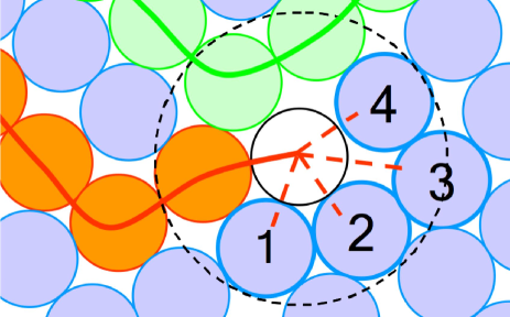
2. Growth: radical (index $i$) randomly chooses one of its first neighbors still in the monomer state (if any available) to create a new covalent bond and increase the local chain length $N_{i}$ of chain $i$. The amount of growth steps $n_{growth}$, defined initially, controls the maximum chain length $N_{i}|_{MAX}=n_{growth}$. Note that this allows us, as mentioned previously, to mimic the polydispersity associated with living polymerisation. This stage of the process is schematically depicted on Fig. 1.

3. Relaxation: this is an essential ingredient of the method. Between two successive growth steps, a radical is allowed to explore its neighborhood during $n_{MDSbg}$ MD steps. This is equivalent to let a chain evolve in the solvent and explore a part of its conformational phase space in situ while polymerization is taking place, hence permitting a partial relaxation.

4. Termination: For polydisperse systems the generation procedure is stopped after a fixed number of growth steps $n_{growth}$. To produce a monodisperse system, the process is stopped only when each chain has reached a desired size $N$, whatever the number of growth steps. Naturally, the time elapsed before termination will depend on the ratio $(N\times M)/N_{monom}$ which we took near $80\%$. Finally the residual monomers (or solvent) are removed and the system is relaxed to reach at constant pressure.

Fig 1: (Color online). Growth step during the radical-like polymerization algorithm. A radical (white) is randomly assigned one of its first monomers neighbors (blue ones, numbered from $1$ to $4$) to create a new covalent bond and increase the local chain length $N_{i}$.

In the following we will be only interested in semi-flexible chains for which no angular potential and bond rigidity are imposed. In principle, such constraints could be included trough a preferential choice of the neighbors during the growth step. Three types of systems were generated using the radical-like polymerization process:

• Cold: pure polydisperse melt. The polymerization procedure involve a finite value $n_{growth}$ of growth steps but without coupling the system to a heat bath by imposing $n_{MDSbg}\equiv 0$, thus preventing any relaxation between growth steps.

• Hot: pure polydisperse melt. The number $n_{growth}$ of growth steps is also fixed to a finite value, but for this kind of polymerization, the system is coupled to a heat bath by fixing a finite number $n_{MDSbg}$ of relaxation steps between each growth step, and setting MD parameters using a Nosé-Hoover barostat with $k_{B}T=2$ and $P=0.5$. For this kind of procedure, the polymerization process is stopped once the number of growth steps is reached.

• HotMono: pure isodisperse melt. For this kind of process, the number of growth steps is infinite. Practically, growth stage occur until all chains reach the desired size $N$. The system is coupled to a heat bath (Nosé-Hoover thermostat and barostat with $k_{B}T=2$ and $P=0.5$) during the relaxation stage. $n_{MDSbg}$ MD steps are performed after each growth step.

In the next section, these three types of generation processes will be tested and compared. The monodisperse HotMono generation procedure will also be compared to the more classical Push-Off techniques Auhl ; Kremer .

Within the Push-Off framework, chains are generated randomly in the simulation box without considering excluded volume Theodorou . Thus, Lennard-Jones interactions for non-bonded monomers cannot be introduced immediately because chains spatially overlap. To bypass this difficulty, modified Lennard-Jones potentials (Slow Push Off), or intermediate soft repulsive potential (Fast Push Off) are then introduced, and eventually replaced by the LJ potential. Due to its relative simplicity, this method has been widely used in the literature to generate monodisperse systems.

We refer to Auhl for details and discussions about FPO technics. In our implementation, the systems generated with FPO ($M=200$ chains with chain length of $N=200$) are relaxed during $10^{7}$ MDS for systems o under Nosé-Hoover thermostat ($k_{B}T=2.0$) and barostat ($P=0.5$).It has to be noticed that this quite easy procedure is known to create significant distortions in the chain statistics on length scales comparable to the tube diameter Auhl ; Brown ; Hoy , requiring thus relatively long relaxation times. Consequently chain length is generally limited to $N<400$.

II.1.2 parameters

The values of the parameters used in our generation processes and subsequent simulation for the three types of protocols are summarized in Tab. 2. For polydisperse systems, e.g. Cold and Hot, the min and max values of the chain length distribution are also quoted in the same table, and will be discussed below.

For monodisperse systems, we also studied the influence of the number of relaxation steps $n_{MDSbg}$ between growth steps on the final static properties of the polymer melt. This parameter can be considered as a control parameter for the exploration of configurational phase space during growth, at a given temperature and pressure.

	$\,\,n_{growth}\,\,$	$\,\,n_{MDSbg}\,\,$	$\,\,M\,\,$	$\,\,N\,\,$	$\langle N\rangle(t\rightarrow\infty)$
Cold	$350$	$0$	$184$	$[50;344]$	$172$
Hot	$6.7\,10^{4}$	$10$	$215$	$[56;390]$	$226$
HotMono	$10^{5}$	$10$	$215$	$200$	$200$
	$10^{5}$	$300$	$215$	$200$	$200$

Tab 2: Parameters used to simulate the different radical-like polymerization processes discussed in text, during the generation stage.

II.1.3 Structural characterization

Three types structural parameters have been investigated to control the state of relaxation of polymer melts:

• the mean gyration radius $\langle r_{g}\rangle$ defined by:

  $$\langle r_{g}\rangle^{2}=\sum_{i=1}^{M}\frac{\sum_{j=1}^{N}\left(\mathrm{r_{j}^{i}}-\langle\mathrm{r^{i}}\rangle\right)^{2}/N^{i}}{M}$$ (3)

  where $\mathrm{r_{j}^{i}}$ is the position of the $j$-th atom of the $i$-th chain, $\langle\mathrm{r^{i}}\rangle$ is the center of mass of chain $i$ and $N^{i}$ is the size of chain $i$.

• the Mean Square Internal Distance (MSID) $\langle\mathrm{r}^{2}\rangle(n)$ is the average squared distance between monomers $j$ and $j+n$ of the same chain. It is defined by:

  $$\langle\mathrm{r}^{2}\rangle(n)=\sum_{i=1}^{M}\frac{\sum_{j=1}^{N^{i}-n}\left(\mathrm{r_{j}^{i}}-\mathrm{r_{j+n}^{i}}\right)^{2}/(N^{i}-n)}{M}$$ (4)

  Note that the MSID $\langle\mathrm{r}^{2}\rangle(n)$ is a function of $n$ and $\langle b^{2}\rangle^{1/2}=\sqrt{\langle\mathrm{r}^{2}\rangle(1)}$ is the mean bond length.

• the primitive path: the Primitive Path Analysis is a powerful tool to investigate the distance between chains entanglements. It is a key parameter, that controls the mechanical or rheological properties of the polymer melt. Section III.3 will be devoted to the PPA.

III Results for a homopolymer melt

III.1 Dynamics of the polymerization process

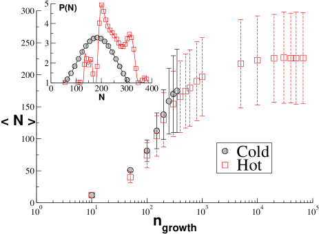
A preliminary study is devoted to the growth dynamics of polydisperse system, namely Hot and Cold methods. In Fig. 2, the mean chain length $\langle N\rangle$ is plotted as a function of the number of growth steps preformed during polymerization. It is worth noting that polydispersity has spontaneously appeared as a result of the growth process. We observe that both methods display the same evolution: a rapid increase followed by a saturation due to the lack of available monomers. However, the Cold procedure is stopped before the Hot one because thermal mobility allows a more efficient exploration of configurational space by the active radicals.

The standard deviation $\sigma_{N}=\sqrt{\langle N^{2}\rangle-\langle N\rangle^{2}}$ is also indicated for both systems with vertical bars centered on respective symbols.

The final size distributions at the end of the generation procedure $P(N)$ are plotted for both systems on inset of Fig. 2. As expected, the peak is shifted towards larger sizes and is slightly narrower for the Hot system.

In our simulations the polydispersity index $I_{p}=M_{w}/M_{n}$, is accessible through the ratio $I_{p}=\langle N^{2}\rangle/\langle N\rangle^{2}$. The final polydispersity index is a little lower for the Hot system (around 1.057) than for the cold system (around 1.103). Again, this is probably due to thermal mobility which allows smaller chains to find new monomers to continue the growth.

Our generation procedure, which is very close to living polymerisation (see section II.1) leads to polydispersity indexes that are reasonably close to experimental ones resulting from living polymerization (typically of order 1.3), which gives us confidence in the physical background our the radical radical-like polymerization algorithm. Moreover, it would be very easy to slightly modify our method to simulate other kind of polymerization processes which would lead to higher polydispersity. Experimental values of polydispersity index can reach a value of 10 or more for classical polymers where coupling, transfert or disproportination are involved (see section II.1).

Fig 2: (Color online) Mean chain length size $\langle N\rangle$ (symbols) and polydispersity index $I_{p}$ (lines) evolution during polymerization stage versus the number of growth step, and for the two Hot and Cold simulated isodisperse systems. Also plotted is the standard deviation $\sigma_{N}$ represented by vertical bars centered on symbols. Inset: Size distribution $P(N)$ for the same systems at the end of the generation procedure.

In order to quantify the evolution of the structural properties of chains during production runs for the Hot, Cold and HotMono methods, we also investigated the evolution of the mean gyration radius $\langle r_{g}(t)\rangle$ normalized by the mean bond distance $\langle b^{2}(t)\rangle^{1/2}$ during the growth (Fig. 3) and relaxation (Fig. 4) stages. Such evolutions are investigated for the three systems ($n_{MDSbg}=10$ for Hot and HotMono during the generation stage - see Tab. 2).

Fig 3: (Color online) Generation stage: evolution of the mean gyration radius $\langle r_{g}(t)\rangle$ normalized by the average bond length $\langle b^{2}(t)\rangle^{1/2}$ and averaged over all chains. Generation exhibits two distinct stages: (i) a pure growth stage characterized by a $t^{\frac{1}{2}}$ growth kinetics; (ii) a saturation stage where gyration radii reach a plateau value. A value of $n_{MDSbg}=10$ has been used for Hot and HotMono methods (see Tab. 2).

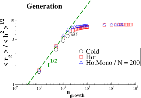
In figure  3, we observe that the generation proceeds in two distinct stages: (i) a pure growth stage characterized by a $t^{\frac{1}{2}}$ growth kinetics; (ii) a saturation stage where gyration radii reach a plateau value. The power law simply means that during stage (i), each growth step is successful and lead to an increase of the chain length $N$: $N\propto n_{growth}$. As $r_{g}\propto N^{\frac{1}{2}}$, we obviously get $r_{g}\propto n_{growth}^{\frac{1}{2}}$.

Fig 4: (Color online) Relaxation stage (e.g. after polymerization): evolution of the mean gyration radius as a function of the number of MD steps necessary to reach a total number $n_{tot}=n_{growth}\times n_{MDSbg}+n_{relax}=10^{7}$ MD steps. Fast Push Off (FPO) and HotMono methods converge to the same value.

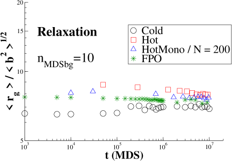
In figure  4, the time evolution of the mean radius of gyration for the Cold, Hot, HotMono and also Fast Push Off (FPO) are compared during the relaxation stage. The radius of gyration is plotted versus the number of MD steps necessary to reach a total number $n_{tot}=n_{growth}\times n_{MDSbg}+n_{relax}=10^{7}$ MD steps. Final values of gyration radii depend on mean chain length $N$: the Cold method, which gives the smallest final mean chain length ($N=172$) leads to the smallest mean gyration radius. Then come the HotMono and the FPO methods, which converge logically to the same gyration radius. Finally, the Hot method, which gives the largest final mean chain length ($N=226$) leads to the largest mean gyration radius.

Fig 5: (Color online) Growth and relaxation stages: evolution of the mean gyration radius as a function of the mean chain size during growth (curves) and relaxation (vertical arrows) stages. Data from KremerKremer are also represented. They predict a $N(t)^{1/2}$ dependance. After the removal of remaining monomers and $10^{7}$ MD relaxation steps, all generation technics are in very good agreement with Kremer’s results.

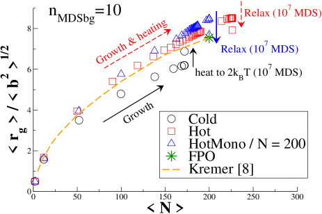
In order to investigate the evolution of the chain size as a function of chain length during the growth and relaxation stages for all polymerization methods, we plotted $\langle r_{g}(t)\rangle/\langle b^{2}(t)\rangle^{1/2}$ versus $\langle N\rangle$ on Fig. 5. In this figure, relaxation process (at constant $N$) is represented by vertical arrows. We also plotted in this figure data from KremerKremer resulting from long time equilibration, which predict a $N^{1/2}$ dependance.

After the removal of remaining monomers and $10^{7}$ MD relaxation steps, all generation methods (Cold, Hot and HotMono) are in very good agreement with Kremer’s target function $\langle r_{g}(t)\rangle/\langle b^{2}(t)\rangle^{1/2}$ versus $\langle N\rangle$.

However, with Cold, Hot or HotMono) (with $n_{MDSbG}=10$), it seems that relatively long relaxation times (up to $10^{7}$ MD steps) are necessary to reach Kremer’s target function. Therefore, in what follows, the effect of the number of MD steps between each growth step ($n_{MDSbG}$) will be investigated.

Fig 6: (Color online) Evolution of the mean radius of gyration as a function of time (in MD steps) during growth and relaxation stages: generation of $M=215$ chains of expected length $N=200$ at $k_{B}T=2$ and $P=0.5$. Two different values of $n_{MDSbG}$ (the number of MD steps between each growth step) are compared. A larger value of $n_{MDSbG}$ slows down the growth kinetics, but leads to better equilibrated systems once growth is completed. For $n_{MDSbG}=300$, no equilibration stage is required to reach the mean radius of gyration obtained with the Fast Push Off (FPO) method.

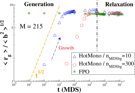
In Fig. 6, the mean normalized radius of gyration is plotted versus simulation time for the generation of $M=215$ chains of expected length $N=200$ at $k_{B}T=2$ and $P=0.5$. Two different values of $n_{MDSbg}$ are investigated: $n_{MDSbg}=10$ and $n_{MDSbg}=300$. It can be observed that a larger value of $n_{MDSbG}$ slows down the growth kinetics, but leads to better equilibrated systems once growth is completed. For $n_{MDSbG}=300$, no equilibration MD steps are required to reach the radius of gyration obtained with the Fast Push Off (FPO) method.

This shows that the chains generated here reach their equilibrium structure more rapidly for the protocole that spends more time during the growth stage, thus pointing out the main interest of this algorithm: i.e. equilibration is occurring during generation, provided an appropriate compromise for the number of MD steps between growth steps is chosen.

III.2 Comparison of chains structure for HotMono and FPO methods

The structure of a polymer melt can be characterized by a wide variety of static or dynamic interchain and intrachain correlation functions Kremer ; Auhl ; Wittmer ; Flory ; deGennes ; Vladkov which are more or less sensitive to the artifacts introduced by the preparation procedure and which equilibrate on different time scales. One may note that for fully flexible chains simulated in our model (only FENE + LJ interactions), i.e. without torsional barrier and bending stiffness potentials, the local monomer packing relaxes quickly, while deviations of chain conformations on large scale require large times to equilibrate.

To validate our generation methods according to more “classical” techniques, we will be interested, in the following, by a measure of internal chain conformation, namely the Mean-Square Internal Distance (MSID) $\langle\mathrm{r}^{2}\rangle(n)$. This function, defined in Eq. (4) above, gives the average squared distance between two monomers belonging to the same chain, and separated by a subchain of $n$ monomers.

Fig 7: (Color online) Mean square internal distance (MSID) of generated melts measured after from long MD runs ($10^{7}$ MD steps). All the simulated systems (Cold, Hot, HotMono and FPO are compared to the target function of AuhlAuhl . Error bars are calculated using standard error function on statistical samples. All methods lead to well equilibrated melts.

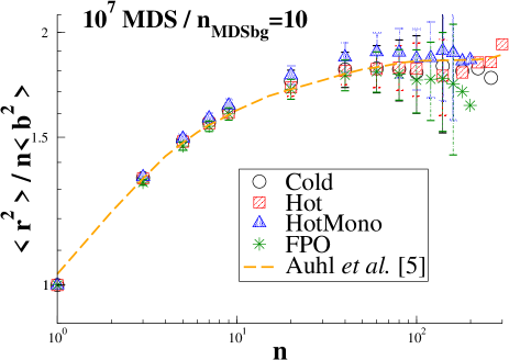
The MSID is shown in Fig. 7 for all simulated systems after the total number of MD steps $n_{tot}=n_{growth}\times n_{MDSbg}+n_{relax}=10^{7}$ MD steps. Cold, Hot, HotMono (with $n_{MDSbg}=10$), and also Fast Push Off (FPO) seem to converge to the same configuration since they all fit nicely with the “target function” defined by AuhlAuhl as the signature of well equilibrated melts.

Error bars in Fig. 7 are estimated using the standard error function that includes the number of subset events taken into account to compute the MSID. As $n$ reaches chain length $N$ ($n\rightarrow N$), less and less pairs of monomers are included in the statistics, leading to large error bars for large $n$. Hence, error bars for large $n$ have not been represented. We thus consider that the values obtained for large $n$ are not statistically significant.

Once again, all our generation methods (Cold, Hot and HotMono) lead to well equilibrated melts (according to the MSID criterion) after (i) generation, (ii) removal of remaining monomers and (iii) $10^{7}$ MD relaxation steps.

Fig 8: (Color online) Mean square internal distance (MSID) of mono-disperse melts. The effect of the number of MD steps between each growth step is studied. A larger value of $n_{MDSbG}$ leads to better equilibrated systems, whom which MSID fits nicely with FPO and the target function of AuhlAuhl .

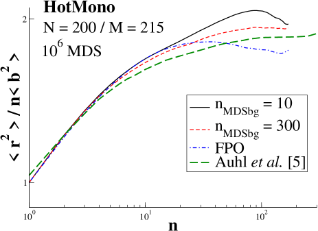
As far as the radius of gyration is concerned, we showed that the number of MD steps between successive growth steps ($n_{MDSbG}$) has an effect on the final structure of the melt. Indeed, the number ($n_{MDSbg}$) of relaxation steps between growth steps can be view as a relaxation process for chains during the polymerization stage. Therefore, the MSID of mono-disperse melts has been investigated for $n_{MDSbg}=10$ and $n_{MDSbg}=300$.

On Fig. 8, MSID resulting from HotMono generation (with $n_{MDSbg}=10$ and $n_{MDSbg}=300$) are compared with MSID resulting from FPO generation and the target function of AuhlAuhl . For all systems, an equilibration stage of $n_{tot}=n_{MDSbg}\times n_{growth}+n_{relax}=10^{6}$ MD steps after generation has been performed. Despite this relatively low equilibration time, it can be observed in Fig. 8 that the HotMono generation method with 300 MD steps between each growth step leads to relatively well equilibrated systems, even slightly better than FPO method. This corroborates previous results from Fig. 6, and points out, once again, the main interest of this radical-like generation method: relaxation takes place while generation is performed.

III.3 Primitive Path Analysis

Entanglements between chains are an important topological feature, that controls many dynamical properties of polymer melts. A practical tool for characterizing entanglements is the Primitive Path Analysis (PPA), which will be the object of this section.

Proposed by EveraersEveraers with the aim of constructing a real space representation of de Gennes’ tube model, the PPA technique is an interesting tool for obtaining informations about the density of entanglements which has not been accessible through other theoretical or direct experimental measurements.

Recently Hoy and Robbins Hoy applied this technique to quantify the effect of the generation procedure and of the relaxation for two types of generation methods, namely the FPO system and the Double-BridgingAuhl relaxation technique. Following their idea, we apply this to our different radical-like generation methods, first focusing on the comparison between HotMono and FPO method.

The principle of PPA is the following:

• We start with any given configuration, during the growth or in the final state, after or before the relaxation step.

• The two chains ends are kept fixed, while the intra-chain pair interaction (covalent bonds) are shifted to get their minimum energy at a zero distance while increasing the bond tension in Eq. (2) to $k=100$;

• To prevent chain crossingSukumaran , weak bonds lengths have been monitored and limited to $1.2\sigma$.

• The system is then equilibrated using a Conjugate Gradient algorithm in order to minimize its potential energy and reach a local minimum.

• The contour length of the primitive path $L_{pp}$ is then the total length of the chain (the sum of all straight primitive path segments length).

If no entanglement exists between chains, $L_{pp}$ should be equal to their end-to-end distance $r_{ee}$. The presence of entanglements leads to $L_{pp}>r_{ee}$ with a typical Kuhn length $a_{pp}=\langle r^{2}_{ee}\rangle/L_{pp}$ and an average bond length $\langle b_{pp}\rangle=L_{pp}/N$. The number of monomers in straight primitive path segments is then given by:

$$N_{pp}(N)=\frac{a_{pp}}{\langle b_{pp}\rangle}=\frac{N\langle R^{2}_{ee}\rangle}{L^{2}_{pp}}$$ (5)

For short chains without any entanglements, the primitive path length equal end-to-end distance leading to $N_{pp}=N$. When chain lengths are comparable to the entanglement length, $N_{pp}<N_{e}$, $N_{e}$ being the real entanglement value. For sufficiently long chains, i.e. $N>2N_{e}$, several entanglements per chains exist, and $N_{pp}(N)=N_{e}$.

Fig 9: (Color online) Evolution of the number $N_{e}(t)$ of monomers in straight primitive path segments along simulation times for isodisperse systems HotMono and FPO. Calculation were performed both during the generation (polydisperse) phase and the relaxation (isodisperse) phase separated by the vertical dashed line. Units of time are in $\tau$ units, i.e. $n_{tot}\times\delta t$. The horizontal line gives value for $N_{e}$ from SukumaranSukumaran .

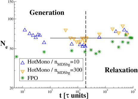
The PPA analysis has been performed at different simulation times (during generation and relaxation stages) and results are shown in figures  9 and 10.

Fig. 9 displays the number of monomers in straight primitive path segments $N_{pp}=N_{e}$ for FPO and HotMono ($n_{MDSbG}=10$ and $n_{MDSbg}=300$) generation methods. The vertical dashed line separates the generation and growth regimes. The horizontal line is the entanglement length $N_{e}$ from SukumaranSukumaran , that is in excellent agreement with our data. This asymptotic value is even reached during the generation stage for the HotMono technique with $n_{MDSbg}=300$: the relaxation stage is not required for this system!

The radical-like method appears to perform perform particularly well at the relaxation stage: the entanglement length do not deviate much from the asymptotic value for the HotMono system in comparison to the FPO method.

Fig 10: (Color online) Ratio $N_{e}(t)/\langle N(t)\rangle$ for polydisperse systems Cold and Hot against simulation time. Dashed (mid-dashed) vertical line separates generation to relaxation stages for the Cold (Hot) method. Also shown is the same ratio from SukumaranSukumaran for chains length $N=200$ as an indicative value.

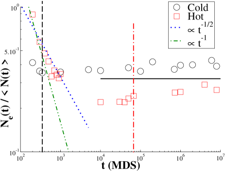
The PPA analysis has also been implemented for polydisperse Hot and Cold systems. Fig. 10 shows the ratio $N_{e}(t)/\langle N(t)\rangle$ for polydisperse systems (Cold and Hot) against simulation time. During the generation stage, the time scale is given in $n_{growth}$ steps units, whereas given in $n_{relax}$ MD steps during the relaxation stage.

For Cold system, generation/relaxation transition is represented by a dashed vertical line, while a dot-dashed line is used for Hot system.

The same indicative value for the entanglement length $N_{e}/N$ from SukumaranSukumaran for chain length of size $N=200$ is also shown, and must be considered as a mean value for both polydisperse systems.

Indeed, the mean chain length at the end of the generation phase for Cold system is $\langle N\rangle_{\textit{Cold}}(t\rightarrow\infty)=172$, while for the Hot $\langle N\rangle_{\textit{Hot}}(t\rightarrow\infty)=226$ (see table  2).

For the Cold method, the investigated ratio is almost constant along the whole relaxation stage, during which entanglements do not vary much.

For the Hot system, this ratio displays a more complex behavior. First, a power law decrease, as noted by dotted ($\propto t^{-1/2}$) and dotted-dashed line ($\propto t^{-1}$), is observed, until $n_{growth}\sim 700$, corresponding to a ratio $N_{e}(t)/\langle N(t)\rangle\sim 1/3$ nearly equal to results from Sukumaran for $N=200$ homopolymer chain melts.

In this regime, $\langle N(t)\rangle$ grows more rapidly than $N_{e}(t)$, and the growth process of each chain interacts with a stochastic background associated with the ensemble of growing chains. Thus, in this Rouse-like regime, topological constraints do not play a significant role and one may expect that chains with average length $\langle N(t)\rangle<N_{e}\sim N/3$ dominate the polymerization, following a Rouse-like chain dynamics.

Following this regime, while $\langle N(t)\rangle$ still grows, a stabilization of the same ratio is observed. In this regime, $N_{e}(t)/\langle N(t)\rangle<1/3$, and a slowing down is observed during chain growth dynamics. This new reptation-like regime, corresponds to a dynamics where the surrounding medium topology limits transverse chains displacements around their own contour length. Chains with mean size $\langle N(t)\rangle>N_{e}\sim N/3$ follow this reptation-like dynamics, and the polymerization process is slowed down. While the longest chains are still growing, the average entanglement length does not vary drastically, as one can see once the generation stage is finished, where the ratio $N_{e}(t)/\langle N(t)\rangle\rightarrow N_{e}/N$.

From all these results, it appears that our approach is validated as a method for generating equilibrated configurations of homopolymer melts. In the following section, the radical-like algorithm will be used to generate block copolymers in a lamellar configuration.

IV Application to copolymer generation

In this section, generation of block copolymers will be investigated and our radical-like polymerization algorithm will be modified to get a lamellar structure.

Modeling the demixion itself is not an easy task. Adjusting force-fields and replicating basic units of previously assembled copolymers, SrinivasSrinivas managed to obtain large scale demixtion in biological systems (self-assembled copolymers in water). ZangZhang used full-atomistic simulations based on dynamics density functional theory but their approach is limited to small system sizes. May be more adapted to block copolymer generation, semi-particle based methods such as Single Chain in Mean-field Muller_2 ; Daoulas ; Sides ; Daoulas_2 seem to be promising.

In the following, we present an alternative method based on an adaptation of the radical-like method to the particular case of symetric AB diblock where $N_{A}=N_{B}$ and $N=N_{A}+N_{B}$. $L_{x}$, $L_{y}$ and $L_{z}$ are the box sizes along the $x$, $y$ and $z$ directions.

Fig 11: (Color online) Snapshots of symmetric di-block copolymers generated using the radical-like co-polymerization method for $M=215$ chains of length $N=200$, and for two values of the Flory-Huggins compatibility parameter $\chi N=396$ (segregation regime - up), and $\chi N=4$ (one phase region: mixing in progress - down).

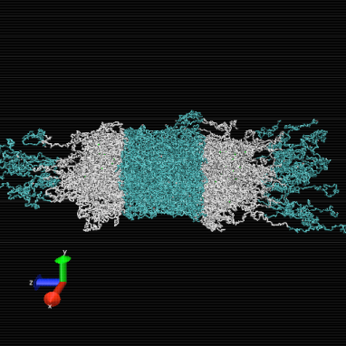
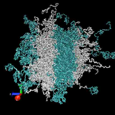
Generation of a di-block copolymer with an interface lying in the ($xy$) plane is performed as follows, starting from a Lennard-Jones liquid of monomers:

1. Nucleation: Each monomer $i$ has a probability $p$ to be a radical of type $A$ if, say, $z_{i}>L_{z}/2$ and B otherwise.

2. Growth: As long as the chain does not reach the size $N/2$ ($N(t)<N/2$), growth is performed as in a homopolymer with a supplementary condition: addition of a new monomer $j$ is possible only if it lies in the same region ($z_{j}>L_{z}/2$ for $A$ chains and $z_{j}<L_{z}/2$ for $B$ chains). The interface situated at $z=L_{z}/2$ is then impermeable: no chain can cross it.

3. From one region to the other: Once a chain reach the critical size $N/2$ ($N(t)=N/2$, the growth within a lamella is stopped. A force is applied to attract the chain ends to the interface, and the condition above is reversed: addition of a new monomer $j$ is possible only if it lies in the opposite region ($z_{j}<L_{z}/2$ for $A$ chains and $z_{j}>L_{z}/2$ for $B$ chains).Under this new condition, and once a radical combines with a new monomer in the opposite region, it turns into the opposite species ($A$ radical becomes $B$ radical and $B$ radical becomes $A$ radical). For chains, with $N(t)>N/2$, the growth is then continued with the impermeable interface condition: addition of a new monomer $j$ is possible only if it lies in the same region ($z_{j}>L_{z}/2$ for $A$ chains and $z_{j}<L_{z}/2$ for $B$ chains). Growth a a chain occurs until its length reach the size $N$.

4. Relaxation: As for homopolymers, a number $n_{MDSbg}$ of MD steps is performed between each growth step, during which the systems is coupled to the heat bath at $k_{B}T=2\epsilon_{\alpha\alpha}$ and $P=0.5$.

With this procedure, all chains have the same length $N=N_{A}+N_{B}$ and $N_{A}=N_{B}$. Systems are then relaxed at $k_{B}T=0.5\epsilon_{\alpha\alpha}$ and $P=0.5$ during $10^{6}$ MD steps.

Values for excluded volume potentials  1 and  2 have been chosen as, $\epsilon_{AA}=\epsilon_{BB}=1.0$ and the interaction with the solvent fixed to $\epsilon_{\alpha s}=1.0$ where $\alpha\in[A,B]$ and $s$ being the solvent molecular type. All $\sigma_{\alpha\beta}=1.0$ while potentials are truncated and shifted at $r_{c}=2.5\sigma_{\alpha\beta}$.

The order-disorder transition temperature is governed by the product of $\chi N$, where $\chi=(\epsilon_{AA}+\epsilon_{BB}-2\epsilon_{AB})/(2k_{B}T)$ is the Flory-Huggins temperature-dependant interaction parameter characterizing the AB incompatibility. Symmetric diblock copolymers are homogeneous at small $\chi N$ value, but strongly heterogeneous with ordered structure when $\chi N$ exceeds, in mean-field theory, the critical order-disorder transition value $\chi N_{ODT}\approx 10$. Hence, as a first application of our radical-like copolymerization algorithm, we simulated such diblock copolymers in the two limiting case of weak segregation limit with $\chi N=4$ (($\epsilon_{AB}=0.99$), and the strong one, with $\chi N=396$ ($\epsilon_{AB}=0.01$).

To observe box dilatation and inter-lamellae distance relaxation, an anisotropic Nosé-Hoover barostat has been used during $5.10^{6}$ MD steps, in such a way that $P_{x}=P_{y}=P_{z}=0$, while the temperature was fixed to $k_{B}T=0.5\epsilon_{\alpha\alpha}$.

Snapshots of diblock configurations are shown in Fig. 11, where simulations have been performed on $M=215$ chains with a polymerization degree of $N=200$. In the upper frame of Fig. 11, one can observe that the interface separating the two blocks is well defined and stable, as expected in the strong segregation limit. On the contrary, in the right panel, the same interface is poorly defined and appears to be unstable on the simulation timescale. One expects the diblock to become homogeneous in the long time limit.

This preliminary study on diblock copolymers allowed us to validate the radical-like copolymerization technics. The advantage of this technique resides in the control of the geometry of simulated copolymers, as well as the possibility to generate in a flexible way configurations with various topologies and chain architectures.

V Conclusion

1. the radical-like polymer chains generation method is inspired by radical polymerisation in which the reactive center of a polymer chain consists of a radical. The free radical reaction mechanism can be divided in to three stages: (i) initiation (creation of free radicals); (ii) propagation (construction of the repeating chain): (iii) termination (radical is no longer active).

2. Performing an relatively important number of MD relaxation steps between each growth step (typically 300) leads to well equilibrated chains (in terms of gyration radii, Mean Square Internal Distance, and Primitive Path Analysis), even for relatively short relaxation stage ($10^{6}$ MD Steps).

3. The main advantage of the radical-like generation algorithm is that equilibration occurs simultaneously as chain growth, within a coarse grained molecular dynamics scheme.

4. Polymer melts generated with the radical-like algorithm are as well equilibrated as melts generated by more classical methods (like fast push-off).

5. The radical-like generation method is particularly adapted to generate polydisperse polymer melts (branched polymers, star polymers, copolymers,…).

6. nano-structured lamellar block copolymers have been successfully generated with the radical-like method.

7. physical and mechanical properties of di-block and tri-block copolymers generated using this algorithm, will be the subject of a futur paper.