Off–diagonal Ground State Properties of a 1D Gas of Fermi Hard Rods

Abstract

A variational Monte Carlo calculation of the one-body density matrix and momentum distribution of a system of Fermi hard rods (HR) is presented and compared with the same quantities for its bosonic counterpart. The calculation is exact within statistical errors since we sample the exact ground state wave function, whose analytical expression is known. The numerical results are in good agreement with known asymptotic expansions valid for Luttinger liquids. We find that the difference between the absolute value of the bosonic and fermionic density matrices becomes marginally small as the density increases. In this same regime, the corresponding momentum distributions merge into a common profile that is independent of the statistics. Non–analytical contributions to the one–body density matrix are also discussed and found to be less relevant with increasing density.

I Introduction

Quantum one–dimensional (1D) systems of bosons and fermions have attracted great attention in the last years, both from the experimental and theoretical points of view Paredes2004 ; Bloch2005 ; Moritz2003 ; Richard2003 ; Khodas2007 ; Khodas2007b . The combined effect of quantum fluctuations and reduced dimensionality produces new and intriguing features different or not present in three-dimensional (3D) systems, as for instance the nonexistence of a true Bose–Einstein condensate in the homogeneous phase (not even at $T=0$).

As in the boson case, quasi–1D systems of fermions are experimentally realized confining to zero point oscillations the radial motion of a 3D trapped cloud of atoms in a largely elongated harmonic trap. This is done acting on the system with two perpendicular laser beams forming a two–dimensional optical lattice. In this setup, the transverse frequency $\omega_{\bot}$ of the harmonic trap is much larger than the longitudinal frequency $\omega_{\|}$, and such that the Fermi energy of the confined gas satisfies the condition $E_{F}=N\hbar\omega_{\|}/2\ll\hbar\omega_{\bot}$. Under these circumstances, an array of quasi–1D systems is created, thus allowing for a statistical evaluation of the most relevant quantities of interest Giorgini2007 .

Due to the Pauli exclusion principle, $s$–wave scattering between atoms of the same spin is not possible. In this way, the low–energy properties of the system are dominated by the interaction between atoms of different spin. In a pseudopotential description, the quasi–1D scattering length of the resulting interaction is directly related to the real 3D scattering length through the expression

$$a_{1D}={a_{\perp}^{2}\over a_{3D}}\left(1-C{a_{3D}\over a_{\perp}}\right)\ ,$$ (1)

with $C=\zeta(1/2)/\sqrt{2}=1.0326$ and $\zeta(\cdot)$ the Riemann zeta function Olshanii1998 .

A peculiarity of the one-dimensional world is that a certain number of exactly solvable many-body systems is known. The ground state energy of a system of bosons with $\delta$-pseudopotential interactions (Lieb-Liniger model) has been obtained Lieb1963 by using a Bethe ansatz solution in all interaction regimes, ranging from the weakly interacting Bose gas to the strongly correlated Tonks-Girardeau limit Girardeau1960 . The ground state energy of a system of particles interacting through a $1/z^{2}$ potential (Calogero-Sutherland model) is also known for both fermions and bosons Sutherland1971 . Contrary to the case of bosons, Fermi statistics preclude atoms from interacting via $\delta$-pseudopotentials, which are commonly used to describe $s$–wave scattering processes. Instead, $\delta$-scattering is permitted between atoms of different spins in a system of two component fermions. Such systems have attracted great interest for a long time. There are two classes of excitations in homogeneous two-component 1D Fermi gases, density and spin modes. In the case of attractive interactions sound waves propagate with a well defined velocity while spin waves exhibit a gap Krivnov1975 . If the attraction is very strong, composite molecules consisting of two fermions of different spin are formed.

Even if the energetic properties of a few 1D systems can be determined exactly, much less is known about the correlation functions. Some short-distance properties (at least the leading terms in a $z\to 0$ expansion) are known for the one- Olshanii2003 , two- Gangardt2003 and three- Cheianov2006 particle correlation functions of the Lieb-Liniger model. The Tonks-Girardeau system is a special case where a finite number of terms in the expansion of the one-body density matrix is enough to provide a meaningful description of this quantity at all distances Lenard1964 . Moreover, it was noted in Refs. Sutherland1971 ; Dyson62 that random matrix theory can be used to describe static density correlators in the Calogero-Sutherland model for certain values of the interaction parameter ($\lambda=1/2,2$ and $1$, the later case being equivalent to the Tonks-Girardeau system).

While the short-range properties of spatial correlators depend explicitly on the shape of the interaction potential, the long-range properties are quite generic and governed by the presence of phonons. The Luttinger model Luttinger1963 describes universal long-range properties of all one-dimensional systems with a phononic (i.e. linear) excitation spectrum at low momenta. The long range description of the main ground state one- and two- particle correlation functions was obtained by Haldane in 1981 Haldane1981 . He described asymptotic series with universal power exponents (i.e. exponents that depend only on the density and the speed of sound) and non-universal series coefficients. All terms of the long-range expansion (with explicit expressions for the coefficients) of the one- Astrakharchik2006 and two- Gangardt2001 particle correlation functions have been obtained using the replica method for the bosonic and the fermionic Calogero-Sutherland model, and for all possible interaction strengths including the Tonks-Girardeau limit.

In spite of the progress achieved in analytical approaches, so far the only systematic way to obtain a complete description of the correlation functions relies on numerical methods. Recently, Monte Carlo methods have been successfully used to obtain these functions for the Lieb-Liniger Astrakharchik2003 and the hard rod models Mazzanti2007 ; Gregory2005 . Moreover, time-dependent Lieb-Liniger correlators have also been obtained using numerical summations of Bethe states Caux2006 . In much the same way, finite temperature correlators for the Lieb-Liniger model have been calculated using density matrix renormalization techniques Schmidt2007 .

In this article we resort to Monte Carlo methods to analyze the most relevant ground state correlation functions of a single component system of fermionic hard rods. We note that while fermions with the same spin can not interact through a $\delta$-pseudopotential due to the Pauli exclusion principle, a hard rod interaction is still permitted and provides the simplest interatomic potential defined by only one parameter $a$ (the size of the hard-rod which equals its scattering length).

II Results

In a preceding paper Mazzanti2007 , the leading ground state properties of a Bose gas of 1D hard rods were analyzed and discussed. In this work we extend this discussion to a population of fully polarized fermions interacting through the same spin–independent potential, namely

$$V_{HR}(z)=\left\{\begin{array}[]{cc}+\infty&\mbox{ for $\mid\!\!z\!\!\mid\leq a$}\\ 0&\mbox{ otherwise \ ,}\end{array}\right.$$ (2)

corresponding to the many–body Hamiltonian

$$H=-{\hbar^{2}\over 2m}\sum_{j=1}^{N}{\partial^{2}\over\partial z_{j}^{2}}+\sum_{i<j}V_{HR}(z_{ij})\ .$$ (3)

Despite the complexity of the interaction, both the ground state wave function and the energy are exactly known. The former is a Slater determinant of plane waves Nagamiya1940 ; Krotscheck1999

$$\Psi_{0}(z_{1},z_{2},\ldots,z_{N})\!\! = \!\!{1\over\sqrt{N!}}{\rm det}\left[{1\over\sqrt{L^{\prime}}}\exp(ip_{k}x_{k})\right]$$

$$= \!\!{2^{N(N-1)/2}\over\sqrt{N!}(L^{\prime})^{N/2}}\prod_{i<j}\sin\left[{\pi\over L^{\prime}}(x_{j}-x_{i})\right]$$

where $N$ is the total number of particles located in a box of length $L$ with periodic boundary conditions. In this expression, $L^{\prime}=L-aN$ is the unexcluded length, while $p_{k}^{\prime}=2\pi n_{k}/L^{\prime}$ with $n_{k}$ an integer in the range $-N$ to $+N$ plays the role of a single–quasiparticle momentum. Additionally, $\{x_{k}=z_{k}-(k-1)a\}$ are a set of reduced coordinates for a given ordering of the true particle coordinates $z_{1}<z_{2}-a<z_{3}-2a<\cdots<z_{N}-a(N-1)$. The ground state energy corresponding to this wave function reads

$${E_{HR}\over N}={\pi^{2}\hbar^{2}n^{2}\over 6m}{1\over(1-na)^{2}}\ ,$$ (5)

with $n=N/L$ the linear density of the system. As happens in the 3D case of hard spheres, the scattering length of the hard rod potential equals the size of the rod, $a_{1D}=a$.

One important consequence of the constrains imposed by the restricted dimensionality in 1D is the fermionization of bosons interacting through diverging potentials, where the strong repulsion between particles mimics the effect of the Pauli exclusion principle. In the particular case of hard rods, this duality is explicitly manifested in the form of $\Psi_{0}$, as in the Bose case the exact ground state wave function becomes the absolute value of the expression in Eq. (II) Girardeau1960 . In this case, therefore, all local quantities depending exclusively on $\mid\!\Psi_{0}\!\mid^{2}$, such as the energy, the static structure factor and the two–particle radial distribution function, are identical for bosons and fermions. However, other quantities not diagonal in configuration space are different due to the symmetry properties of $\Psi_{0}$. In this work, we analyze two of the most relevant non–diagonal ground state quantities, namely the one–body density matrix

$$\rho_{1}(z)=N{\int dz_{2}\cdots dz_{N}\Psi_{0}(z,z_{2},\ldots,z_{N})\Psi_{0}(0,z_{2},\ldots,z_{N})\over\int dz_{1}dz_{2}\cdots dz_{N}\Psi_{0}^{2}(z_{1},z_{2},\ldots,z_{N})}\ .$$ (6)

and its Fourier transform, the momentum distribution

$$n(k)={1\over 2\pi n}\int dze^{ikz}\rho_{1}(z)\ .$$ (7)

Both quantities have been evaluated via Monte Carlo sampling of the ground state wave function in Eq. (II) for a number of fermions $N$ between 125 and 1001, located in a box of length $L$ with periodic boundary conditions. Notice that since we use the analytical solution corresponding to the ground state of the Hamiltonian (3), the results of the simulation are exact in a statistical sense.

The one–body density matrix satisfies the condition $\rho_{1}(0)/n=1$, which is a direct consequence of translational invariance and normalization. In the absence of a Bose–Einstein condensate, $\rho_{1}(z)$ decays to zero at large distances. For a system of fermions with a non–positive definite wave function, $\rho_{1}(z)$ changes sign with increasing distance. This is the case for instance of the 1D free Fermi gas, where one has in the thermodynamic limit

$$\rho_{1D}^{FFG}(z)={\sin(\pi nz)\over\pi z}\ ,$$ (8)

with an infinite number of nodes located at the points $z_{m}=m/n$ with $m$ an integer. In the HR system at low densities, the average distance between particles is much larger than the rod size and the net effect induced by the potential is equivalent to a point-like boundary condition. In this limit $\Psi_{0}$ approaches the ground state wave function of the 1D free Fermi gas (as can be easily checked from Eq. (II) setting $a\to 0$), and therefore $\rho_{1}(z)\approx\rho_{1D}^{FFG}(z)$.

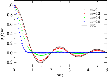
The one–body density matrix $\rho_{1}(z)$ at the particle densities $an=0.1,0.2,0.4$ and $0.6$ (pluses, crosses, stars and squares) is compared with $\rho_{1D}^{FFG}(z)$ (solid line) in Fig. 1. As it can be seen, little differences between $\rho_{1}(z)$ and $\rho_{1D}^{FFG}(z)$ arise at densities lower than $an\approx 0.1$. As the density increases, the main structure of the low–density $\rho_{1}(z)$ is kept while the strength at every point is depressed compared with $\rho_{1D}^{FFG}(z)$. At intermediate and high densities $na\gtrsim 0.5$ the oscillations are no longer visible at the scale of Fig. 1, and essentially all of the strength of $\rho_{1}(z)$ is located around the origin. It is also worth to notice from the figure that the nodal structure of the one–body density matrix is poorly affected by particle correlations, keeping the nodes of $\rho_{1}(z)$ remarkably close to those of $\rho_{1D}^{FFG}(z)$.

Figure 1: (Color online) $\rho_{1}(z)$ at the rod densities $na=0.1$, $0.2$, $0.4$ and $0.6$ (blue pluses, red crosses, green stars and blue squares) compared with the one–body density matrix of the 1D free Fermi gas (solid line.)

The one–body density matrix of any fermionic Luttinger liquid (as hard rods) admits the following asymptotic expansion valid at large distances $z\gg n^{-1}$ Haldane1981

$${\rho_{1}(z)\over n}={1\over(n\mid\!\!z\!\!\mid)^{1/\eta}}\sum_{m=0}^{\infty}{F_{m}\sin\left[2\pi n\left(m+{1\over 2}\right)\!\mid\!\!z\!\!\mid\right]\over(n\mid\!\!z\!\!\mid)^{(m+{1\over 2})^{2}\eta}}\,$$ (9)

where $\eta=2K$ and $K=\pi\hbar n/mc$ is the Luttinger parameter written in terms of the sound velocity $c$. The coefficients $F_{m}$ and the value of $\eta$ change with the interaction and are therefore model–dependent. For a free Fermi gas $\eta=2$, $F_{0}=1/\pi$ and $F_{m>0}=0$. Apart from a few remarkable cases Lenard1964 ; Astrakharchik2006 , these coefficients are, in general, unknown. For a system of hard rods, bosons or fermions, $\eta=2(1-an)^{2}$ which is positive and decreases from $2$ to $0$ with increasing density $an\in[0,1]$. High order terms in Eq. (9) turn out to be then less relevant at large distances, and the asymptotic behavior of $\rho_{1}(z)$ when $z\to\infty$ is therefore dominated by the $m=0$ term. This term cancels at the nodes of $\rho_{1D}^{FFG}(z)$, that is, at the positions $\{z_{m}=m/n\}$. At these points all other terms in the series vanish too, and the whole expression is zero. This fact explains why the nodes of $\rho_{1}(z)$ and $\rho_{1D}^{FFG}(z)$ are so close. Still, Eq. (9) is an asymptotic expansion valid only beyond some healing distance, and therefore the first nodes of $\rho_{1D}(z)$ can deviate from those of $\rho_{1D}^{FFG}(z)$. This effect is small even at large densities and can hardly be appreciated in the $an=0.4$ case of Fig. 1.

Another relevant aspect concerning the structure of the one–body density matrix of a fermionic system of hard rods is manifested when $\rho_{1}(z)$ is compared with $\rho_{1B}(z)$, the one–body density matrix of a system of boson hard rods of the same length and mass, and at the same density. Notice that $\rho_{1B}(z)$ is built as in Eq. (6) but starting from the corresponding bosonic hard rod ground state wave function, which is nothing but the absolute value of the wave function $\Psi_{0}(z_{1},z_{2},\ldots,z_{N})$ of Eq. (II) Mazzanti2007 . Figure 2 displays the absolute value of $\rho_{1}(z)$ compared with $\rho_{1B}(z)$ (which is positive definite) for two particle densities $an=0.2$ and $an=0.6$ (upper and lower panels, respectively). As it can be seen from the figure, both functions share a common short-distance behavior. It is easy to see from the symmetry of the one–body density matrix and the definition of the momentum distribution in Eq. (7) that the leading $z\to 0$ behavior of $\rho_{1}(z)$ and $\rho_{1B}(z)$ is equal and given by

$${\rho_{1}(z)\over n}=1-{\pi^{2}n^{2}\over 6(1-an)^{2}}z^{2}+{\mathcal{O}}(z^{4})\ ,$$ (10)

where the coefficient of $z^{2}$ is proportional to the kinetic energy per particle which, for a system of hard rods (bosons or fermions), equals the total energy in Eq. (5). The prediction of Eq. (10) is shown as a dashed line in Fig. 2 for the two densities analyzed. Clearly, the quadratic approximation is too crude to describe $\rho_{1}(z)$ but at very short distances. A better approximation is obtained when a truncated cumulant expansion is considered instead

$${\rho_{1}(z)\over n}\approx\exp\left[-{\pi^{2}n^{2}\over 6(1-an)^{2}}\,z^{2}\right]\ ,$$ (11)

which is also displayed in the upper and lower panels of Fig. 2 with a solid line. As can be seen from the figure, the cumulant approximation works well both at low and high densities up to approximately the first node of $\rho_{1}(z)$. Beyond that point the approximation certainly breaks down because cumulant expansions can only be carried out on positive defined functions while $\rho_{1}(z)$ changes sign. In this sense, Eq. (11) is a better approximation to $\rho_{1B}(z)$, although visible differences remain in the tails when plotted in logarithmic scale. At intermediate and high densities, however, there is no practical distinction between the fermionic and bosonic cases since the strength in $\rho_{1}(z)$ after the first oscillation is remarkably low. This is seen also in the inset of Fig. 2, where the dashed line is the cumulant approximation while $\rho_{1}(z)$ and $\rho_{1B}(z)$ are displayed with a solid line and can not be distinguished from each other.

Figure 2: (Color online) Absolute value of the one-body density matrix in logarithmic scale at the particle densities $na=0.2$ and $an=0.6$ (upper and lower panel, respectively). Black circles stand for fermions, red squares for bosons. The dashed and solid lines represent the approximations reported in Eqs. (10) and (11). Inset: $\rho_{1}(z)/n$ compared with the truncated cumulant expansion of Eq. (11) (solid and dashed lines, respectively).

At distances larger than the position of the first node, $\rho_{1}(z)$ and $\rho_{1B}(z)$ differ more significantly, specially at low densities. However, at large densities $\mid\!\rho_{1}(z)\!\!\mid$ and $\rho_{1B}(z)$ are almost identical as seen from the figure, the main difference between the two functions being that $\rho_{1B}(z)$ is always positive while $\rho_{1}(z)$ changes sign each time a node is crossed.

This striking fact can be understood by direct inspection of the particle configurations contributing to the one–body density matrix. By definition, $\rho_{1}(z)$ is related to the probability of destroying a particle at the origin and creating a new one at a distance $z$, as given by $\langle\Psi^{\dagger}(z)\Psi(0)\rangle$ with $\Psi$ and $\Psi^{\dagger}$ field operators. In first quantization, $\rho_{1}(z)$ measures the overlap between the wave functions corresponding to different particle configurations where one particle has shifted its position by an amount $z$ (see Eq. (6)) while all other particles are kept in their original positions. Clearly, the different symmetry properties of the Fermi and Bose wave functions can make the contribution of these configurations to the one–body density matrix be of different sign.

A remarkable property of 1D systems like the one analyzed in this work is the fact that the different particle configurations can be classified in $N!$ disjoint subspaces, according to the ordering of the particles. In this way, one can attach labels 1 to $N$ to the particles of a given configuration, and build all other subspaces by sorting the particles in a different order. One can then move from the original subspace $\Omega_{0}$ to any other subspace $\Omega_{\alpha}$ by transposition of particle coordinates. In the Bose case, the wave function is always positive. In the Fermi case, however, moving from one subspace to another implies a change in sign equal to $(-1)^{P}$, where $P$ is the parity of the permutation that leads to that subspace starting from the coordinate ordering of $\Omega_{0}$.

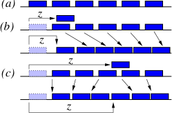
Now consider the high density limit for a system of hard rods. Given the wave function (II), the most probable configuration is one where all particles are equally spaced. Each rod of size $a$ has, in average, a space $l=L/N$ available. At high densities, $l$ is only slightly larger than $a$ and there is not enough room for a particle to be placed between two other particles. In this sense, the most probable configuration will not contribute to $\rho_{1}(z)$ when $z$ is larger than $l$, as schematically represented in Fig. 3a. The only configurations in subspace $\Omega_{0}$ contributing to $\rho_{1}(z)$ are those less probable were particles are more packed as in Fig. 3b, making room for the movement of the selected particle. Belonging to $\Omega_{0}$, these configurations have always positive sign since no particle reordering is required, and contribute the same for bosons and fermions. Of course, this mechanism is only possible at short distances and that explains why the low $z$ behavior of $\rho_{1}(z)$ and $\rho_{1B}(z)$ is equal.

As the distance $z$ increases, the contribution from $\Omega_{0}$ to $\rho_{1}(z)$ becomes negligible and the main contributions come from movements involving a change from $\Omega_{0}$ to different subspaces $\Omega_{\alpha}$. As before, and depending on the density, it may happen that the most probable configuration can not contribute due to the lack of available space, but there are configurations in other subspaces were only the movement of a few particles with respect to the equally spaced configuration is involved, as shown in Fig 3c. These are the most probable ones and produce the major contributions to the one–body density matrix. These contributions have a sign $(-1)^{P}$ for fermions and $+1$ for bosons. At high densities, only one subspace $\Omega_{\alpha}$ contribute significantly, and therefore all contributions have the same sign. If this sign is negative, that leads to a total contribution to the one–body density matrix that is positive for bosons and negative for fermions but equal in absolute value. That explains the observed behavior shown in the lower panel of Fig. 2.

It is also clear from the above arguments that this phenomenon does not happen at low densities, since in this case many different particle configurations have non-negligible contributions for a given $z$, and even at large distances configurations from different $\Omega_{\alpha}$ subspaces contribute. In the Bose case all these configurations have the same sign, while in the Fermi one some are positive and others are negative, leading to a total contribution that is noticeably different for bosons and fermions.

Figure 3: (Color online) Three different configurations contributing to $\rho_{1}(z)$. (a) shows the most probable configuration where all particles are equally spaced. In (b) one particle is displaced a distance $z$, but there is not enough room for it to be placed between two other rods. The only configurations in $\Omega_{0}$ that allow this are ones were many particles have been shifted to close positions, and these are much less probable at high densities. In (c) the displacement $z$ is large and that can only be done moving from $\Omega_{0}$ to another $\Omega_{\alpha}$, that is, changing the order of the particles with respect to the original ordering.

The form of the exact wave function (II) is quite peculiar as the long-range decay of the two-body term $\sin(\pi x/L^{\prime})$ is very “weak”. In this way, correlations between particles are “strong” even at large distances of the order of the box size. This situation should be contrasted with two- or three- dimensional systems, where the two-body Jastrow factor is significantly different from 1 only at short distances Reatto1967 . As a consequence of strong correlations, density matrix $\rho_{1}(z)$ of the HR system does not saturate to a constant value, but decreases as $z$ increases. This is the reason of the absence of a true BEC in the one-dimensional system of hard rods, even at zero temperature. Furthermore, it is also easy to understand that the decay is greatly enhanced in the high-density regime. Indeed, as we see, contributions to the off-diagonal $|z|\gg n^{-1}$ elements of the one-body density matrix at high density come mainly from the scenario described in Fig. 3c. The higher the density, the higher the cost of moving particles in order to make enough room for the displaced particle, and the smaller the weight of such a contribution. As a result $\rho_{1}(z)$ decays faster at higher densities.

Being the one–body density matrix an even function of its argument, the momentum distribution (its Fourier transform, see Eq. (7)) is also even $n(-k)=n(k)$. Consequently and as originally pointed out by Sutherland Sutherland1992 , all odd moments of $n(k)$ are zero. Moreover, $\langle k^{2n}\rangle$ can be written in configuration space as the expectation value of $\langle\sum_{j}\!\!\mid\!\!\partial^{n}\Psi/\partial z_{j}^{n}\!\!\!\mid^{2}\rangle$ once an integration by parts is carried out, and this is independent of the sign of the wave function. Consequently, all finite moments of $n(k)$ are equal for Fermi and Bose hard rods. If $\rho_{1}(z)$ and $\rho_{1B}(z)$ were analytic functions of their arguments and the corresponding momentum distributions had non–divergent moments $\langle k^{2m}\rangle<+\infty$ for all integer $m\geq 0$, then $\rho_{1}(z)$ and $\rho_{1B}(z)$ would be equal, which is not the case. This can happen if only a finite number of moments of the momentum distributions exist, or if the one–body density matrices have non–analytic contributions. In the case of hard rods, both things happen. On one side the interatomic potential is a source of non–analyticity to the wave function, due to the excluded length which makes $\Psi_{0}(z_{1},\ldots,z_{N})$ and all its derivatives be zero when two or more rods overlap, both for fermions and bosons. We thus see that for fixed coordinates $z_{2}$ to $z_{N}$, $f_{z_{2},\cdots,z_{N}}(z_{1})=\Psi_{0}(z_{1},z_{2},\ldots,z_{N})$ is a non–analytic function of $z_{1}$, and one integrates $f_{z_{2},\cdots,z_{N}}(z)$ to get the one-body density matrix.

Notice the non–analyticity of $\rho_{1}(z)$ is an effect produced by the interatomic potential, and thus it is expected to apply both to the Bose and to the Fermi cases. In the $an\to 0$ limit the potential reduces to a point-like interaction with well known properties. For bosons, the system enters the Tonks–Girardeau regime Girardeau1960 . For fermions, the effect of the potential is already taken into account by the antisymmetry of the wave function, and the system behaves as a 1D free Fermi gas. In the later case, the corresponding momentum distribution is $n_{1D}^{FFG}(k)=\theta(k_{F}-k)$ and all moments exist. On the contrary, in the Tonks–Girardeau limit $n(k)$ presents a $1/\!\!\mid\!\!k\!\!\mid^{4}$ large-$k$ tail that makes all moments $\langle k^{m}\rangle$ with $m>3$ diverge Olshanii2003 . The same conclusions about the relevance of the statistics can be drawn when the 1D free Bose gas, with $n(k)\propto\delta(k)$ and all moments equal to 0, is compared with its fermionic counterpart (Fermionic Tonks Girardeau), which has a momentum distribution $n(k)=1/[1+(k/2)^{2}]$ Girardeau2006 . Furthermore, the behavior of the momentum distribution of other exactly solvable 1D models describing interacting Luttinger liquids can be related to the hard rod system though the value of the Luttinger parameter. For instance, in the Calogero–Sutherland model Sutherland1971 with an interatomic potential of the form

$$V(z)={\lambda(\lambda-1)\pi^{2}\over L^{2}\sin^{2}(\pi z/L)}\ ,$$ (12)

the momentum distribution for bosons and fermions decays to zero at large momentum according to a $1/\!\mid\!k\!\mid^{2+2\lambda}$ law Astrakharchik2006 , and thus only a finite number of moments of $n(k)$ exist. Apparently, therefore, the inclusion of an interatomic potential in a 1D system leads to a power-law decay in $n(k)$ that makes it possible for the bosonic and the fermionic systems to have different momentum distributions while sharing all existing moments. Unfortunately, checking this feature from a Monte Carlo simulation is very difficult due to the enhancement of the statistical noise in the tail of $n(k)$ when the order $m$ of the moment $\langle k^{m}\rangle$ increases.

Figure 4: (Color online) Momentum distribution of the gas of Fermi hard rod at different densities (upper panel). From top to bottom at low $k$: $an=0.3$ (black circles), $an=0.4$ (red squares), $an=0.5$ (green diamonds) and $an=0.6$ (blue stars). The lower panel displays $n(k)$ at $na=0.3$ for different number of particles: $N=125$ (black diamonds), $N=251$ (red squares), and $N=1001$ (blue circles).

In higher dimensions, the zero temperature momentum distribution $n(k)$ of a normal Fermi liquid presents a gap at $|k|=k_{F}$ that is inversely proportional to the effective mass at the Fermi surface Pines66 . This gap is also present in the 1D Free Fermi gas. In 1D, however, even weak particle correlations break down this picture. This is the case of Luttinger liquids Luttinger1963 where Haldane theory applies. The Fourier transform of the leading ($m=0$) term in the asymptotic expansion reported in Eq. (9), which oscillates with frequency $k_{F}=\pi n$, reveals that $n(k)$ is continuous at $k=\pm k_{F}$ when $1/\eta+\eta/4\geq 1$. For hard rods, where $\eta=2(1-an)^{2}$ and $an\in[0,1]$, this condition is always met. In this way, the momentum distribution of the hard rod system of fermions is continuous at $k=\pm k_{F}$ at all densities. Furthermore, the same analysis indicates that the slope of $n(k)$ at these points is infinite and negative when $1/\eta+\eta/4<2$. Once again, for hard rods this condition implies the existence of a threshold density $n_{c}a=1-\sqrt{2-\sqrt{3}}\approx 0.48$ below which $dn(k)/dk$ at $|k|=k_{F}$ diverges.

Figure 5: (Color online) Momentum distribution of the gas of Fermi (black squares) and Bose (red circles) hard rod at different densities. The blue dashed line in the lower panel shows the momentum distribution associated to the gaussian one–body density matrix of Eq. (11).

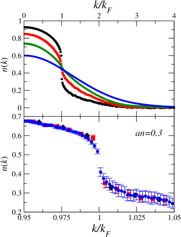
These two aspects are illustrated in the upper and lower panels of Fig. 4. The upper plot shows the momentum distribution $n(k)$ of the system at the particle densities $an=0.3,0.4,0.5$ and $0.6$. As can be seen, the behavior of $n(k)$ at $|k|=k_{F}$ changes with the density, with steeper slope as the density decreases. These results are compatible with an infinite derivative at $|k|=k_{F}$ for the densities $an=0.4$ and $an=0.3$. In any case, the present simulations have been carried out for an even number of particles in order to prevent the ground state from being degenerate. Since $k_{F}=\pi n=\pi N/L$, with a momentum spacing $\Delta k=2\pi/L$ imposed by the use of periodic boundary conditions, no point falls exactly at $|k|=k_{F}$. As a consequence, one can only investigate the behavior of the momentum distribution at the Fermi momentum by increasing the number of particles in the simulation. The lower plot in Fig. 4 shows $n(k)$ around $k_{F}$ for $an=0.3$, as a function of the number of particles in the simulation, for the three values $N=125,251$ and $1001$. As it can be seen from the figure, the points closer to $k_{F}$ corresponding to the highest $N$ seem to confirm the theoretical prediction of a continuous $n(k)$ at that point, while the results obtained at lower $N$, with a coarser spacing, could lead to the wrong conclusion that there is a gap in $n(k)$ at $k=\pm k_{F}$.

We conclude the results section comparing the momentum distribution of the Fermi and Bose systems of hard rods as a function of the density. Figure 5 shows $n(k)$ at the rod densities $an=0.3,0.5$ and $0.7$ (upper, middle and lower panels, respectively). As expected, the momentum distributions are quite different at low densities, as in this limit the fermionic system approaches the 1D free Fermi gas prediction while the bosonic one reproduces the Tonks–Girardeau limit. As the density increases, however, both functions are smeared out and the differences become less relevant, to the point that both curves overlap and can not be distinguished from each other at the highest density considered $an=0.7$. We have also checked numerically that the lowest order moments $\langle k^{0}\rangle$ and $\langle k^{2}\rangle$, the former being a normalization factor and the later the kinetic energy per particle (which equals the total energy per particle for hard rods), are the same for bosons and fermions at the three densities reported in the figure. Additionally and for $an=0.7$, Fig. 5 shows with a dotted line the Fourier transform of the gaussian one–body density matrix of Eq. (11), which is also gaussian.

It is clear from Fig. 5 that the low density momentum distributions of both bosons and fermions are far from being gaussian, but also that the differences between $n(k)$ and $n_{B}(k)$ reduce when the density increases. Furthermore, $n(k)$ and $n_{B}(k)$ seem to approach a common profile that looks gaussian at low momenta, but this happens at even higher densities. This means that in the high density limit the contribution of the non–analytical parts of $\rho_{1}(x)$ is less relevant, and also that in this limit the coefficients in the Taylor expansion of the analytical part of $\rho_{1}(x)$ are mostly dominated by the kinetic energy per particle, according to the cumulant expansion of Eq. (11). It is also apparent from the figure that the differences between the statistics vanish, as a function of the density, before the common profile is approached. Still, one can not deduce from the simulation the analytical form of the large-$k$ behavior of the momentum distributions, and in particular whether a true gaussian is reached when $an\to 1$.

III Summary and Conclusions

In summary, we have studied the one–body density matrix and momentum distribution of a Fermi gas of hard rods, comparing them to their bosonic counterparts. We find that $\rho_{1}(z)$ has a nodal structure quite close to that of the 1D free Fermi gas, in agreement with Haldane’s theory of Luttinger liquids. We have also discussed the analytical properties of $\rho_{1}(z)$ to find that non–analytical parts become less relevant as the density increases. Our numerical simulations confirm that the momentum distribution does not present a sharp gap at the Fermi surface, but has infinite derivative at $k=\pm k_{F}$ when the density is lower than a critical value $an_{c}=1-\sqrt{2-\sqrt{3}}\approx 0.48$. Furthermore, $n(k)$ for fermions and bosons share the same lower order moments while showing an overall fairly different shape. These differences reduce when the density increases, and remarkably the Bose and Fermi momentum distributions approach a common limit at high densities.