Quantum phases of Fermi-Fermi mixtures in optical lattices
Abstract
The ground state phase diagram of Fermi-Fermi mixtures in optical lattices is analyzed as a function of interaction strength, population imbalance, filling fraction and tunneling parameters. It is shown that population imbalanced Fermi-Fermi mixtures reduce to strongly interacting Bose-Fermi mixtures in the molecular limit, in sharp contrast to homogeneous or harmonically trapped systems where the resulting Bose-Fermi mixture is weakly interacting. Furthermore, insulating phases are found in optical lattices of Fermi-Fermi mixtures in addition to the standard phase-separated or coexisting superfluid/excess fermion phases found in homogeneous systems. The insulating states can be a molecular Bose-Mott insulator (BMI), a Fermi-Pauli insulator (FPI), a phase-separated BMI/FPI mixture or a Bose-Fermi checkerboard (BFC).
pacs:
03.75.Hh, 03.75.Ss, 05.30.FkI Introduction
In recent experiments, superfluidity of ultracold 6Li Fermi atoms with population imbalance was investigated in gaussian traps from the Bardeen-Cooper-Schrieffer (BCS) to the Bose-Einstein condensation (BEC) limit mit ; rice ; mit-2 ; rice-2 . In contrast to the crossover physics found in population balanced systems leggett ; nsr ; carlos ; jan , a phase transition from superfluid to normal phase as well as phase separation were observed bedaque ; pao ; sheehy . More recently, experimental evidence for superfluid and insulating phases has also been reported with ultracold 6Li atoms in optical lattices without population imbalance mit-lattice , after overcoming some earlier difficulties of producing Fermi superfluids from an atomic Fermi gas or from molecules of Fermi atoms in optical lattices inguscio ; modugno ; kohl ; stoferle ; bongs .
Before and after experiments, the possibility of interesting phases in population imbalanced ultracold fermions have attracted intense theoretical interest bedaque ; pao ; sheehy ; torma ; pieri ; yi ; silva ; haque ; iskin-mixture ; lobo ; liu-mixture ; mizushima ; parish ; iskin-mixture2 . These works were focused on homogeneous or harmonically trapped Fermi superfluids, where the number of external control parameters is limited. For instance, in addition to population imbalance and scattering parameter , several other experimental parameters can be controlled in optical lattices such as the tunneling matrix element between adjacent lattice sites, the on-site atom-atom interactions , the filling fraction , the lattice dimensionality and the tunneling anisotropy bloch-review . Therefore, optical lattices may permit a systematic investigation of phase diagrams and correlation effects in Fermi systems as a function of , , , and , which has not been possible in any other atomic, nuclear and/or condensed matter systems.
Arguably, one-species or two-species fermions loaded into optical lattices are one of the next frontiers in ultracold atom research because of its greater tunability. The problem of one-species population balanced fermions in lattices has already been studied in the BCS and BEC limits nsr ; micnas ; iskin-prb , while recent works on population and/or mass imbalanced Fermi-Fermi mixtures in lattices were limited only to the BCS regime liu-lattice ; torma-lattice ; chen . In this manuscript, we extend our previous work describing balanced fermions and their s-wave and p-wave superfluid phases in optical lattices iskin-prb , and extend our recent Letter iskin-lattice describing superfluid and insulating phases of Fermi-Fermi mixtures in optical lattices. We discuss specifically the population balanced and imbalanced Fermi-Fermi mixtures of one-species (e.g. 6Li or 40K only) and of two-species (e.g. 6Li and 40K; 6Li and 87Sr; or 40K and 87Sr), as a function of , and for fixed values of in optical lattices and throughout the BCS to BEC evolution. We also pay special attention to the emergence of insulating phases in the strong attraction (molecular) limit. The existence of insulating phases in optical lattices should be contrasted with its absence in homogeneous or harmonically trapped systems pao ; sheehy ; iskin-mixture ; iskin-mixture2 . Furthermore, the present extention to two-species mixtures is timely due to very recent experimental work on 6Li and 40K mixtures dieckmann-lik ; grimm-lik in harmonic traps, which have opened the possibility of trapping these mixtures in optical lattices as well.
Our main results are as follows. Using an attractive Fermi-Hubbard Hamiltonian to describe one-species or two-species mixtures, we obtain the ground state phase diagram containing normal, phase-separated and coexisting superfluid/excess fermions, and insulating regions. We show that population imbalanced Fermi-Fermi mixtures reduce to strongly interacting (repulsive) Bose-Fermi mixtures in the molecular limit, in sharp contrast with homogenous systems where the resulting Bose-Fermi mixtures are weakly interacting pieri ; iskin-mixture ; iskin-mixture2 . This result is a direct manifestation of the Pauli exclusion principle in the lattice case, since each Bose molecule consists of two fermions, and more than one identical fermion on the same lattice site is not allowed for single band systems. This effect together with the Hartree energy shift lead to a filling dependent condensate fraction and to sound velocities which do not approach to zero in the strong attraction limit, in contrast with the homogeneous case iskin-mixture2 . Lastly, several insulating phases appear in the molecular limit depending on the filling fraction and population imbalance. For instance, we find a molecular Bose-Mott insulator (superfluid) when the molecular filling fraction is equal to (less than) one for a population balanced gas where the fermion filling fractions are identical. When the filling fraction of one type of fermion is one and the filling fraction of the other is one-half (corresponding to molecular boson and excess fermion filling fractions of one-half), we also find either a phase-separated state consisting of a Fermi-Pauli insulator (FPI) of the excess fermions and a molecular Bose-Mott insulator (BMI) or a Bose-Fermi checkerboard (BFC) phase depending on the tunneling anisotropy .
The rest of the manuscript is organized as follows. After introducing the Hamiltonian in Sec. II, first we derive the saddle point self-consistency equations, and then analyze the saddle point phase diagrams at zero temperature in Sec. III. In Sec. IV, we discuss Gaussian fluctuations at zero temperature to obtain the low energy collective excitations, and near the critical temperature to derive the time-dependent Ginzburg-Landau (TDGL) equations. In Sec. V, we derive an effective Bose-Fermi action in the strong attraction limit, and describe the emergence of insulating BMI, BFC and separated BMI/FPI phases, and in Sec. VI we suggest some experiments to detect these insulating phases. A brief summary of our conclusions is given in Sec. VII. Lastly, in App. A and B, we present the elements of the inverse fluctuation matrix, and their low frequency and long wavelength expansion coefficients at zero and finite temperatures, respectively.
II Lattice Hamiltonian
To describe mixtures of fermions loaded into optical lattices, we start with the following continuum Hamiltonian in real space
| (1) | |||||
where [] field operator creates (annihilates) a fermion at position with a pseudo-spin , mass and chemical potential . Here, is the optical lattice potential, is the density operator, and describes the density-density interaction between fermions. We allow fermions to be of different species through , and to have different populations controlled by independent , where the pseudo-spin labels the trapped hyperfine states of a given species of fermions, or labels different types of fermions in a two-species mixture. The optical lattice potential has the form where is proportional to the laser intensity, is the wavelength of the laser such that is the size of the lattice spacing, and corresponds to the th component of . This potential describes a cubic optical lattice since the amplitude and the period of the potential is the same in all three orthogonal directions. Furthermore, we assume short-range interactions and set , where is the strength of the attractive interactions.
For this Hamiltonian, the single particle eigenfunctions are Bloch wave functions, leading to a set of Wannier functions that are localized on the individual lattice sites wannier . Therefore, we expand the creation and annihilation field operators in the basis set of these Wannier functions of the lowest energy states of the optical potential near their minima, such that and where () site operator creates (annihilates) a fermion at lattice site with a pseudo-spin . Here, is position of the lattice site . Multi-bands are important when the interaction energy involved in the system is comparable to the excitation energies to the higher bands, and these effects can be easily incorporated into our theory. Notice that, for a complete set of Wannier functions such that the field operators as well as site operators obey the Fermi anti-commutation rules, where is the delta function and is the Kronecker-delta.
This expansion reduces the continuum Hamiltonian given in Eq. (1) to a site Hamiltonian
| (2) | |||||
where is the tunneling amplitude between sites and , is the elements of strength of attractive density-density interactions between sites and , and In this manuscript, we allow tunneling and interactions up to the nearest-neighbors, and choose and respectively. Here, and are strengths of the on-site and nearest-neighbor interactions, respectively. This reduces the general site Hamiltonian given in Eq. (2) to a nearest-neighbor site Hamiltonian
| (3) | |||||
where restricts sums to nearest-neighbors only such that . This is the nearest-neighbor Fermi-Hubbard Hamiltonian for a simple cubic lattice.
Finally, we Fourier transform the site operators to the momentum space ones, such that and where is the number of lattice sites, and () operator creates (annihilates) a fermion at momentum with a pseudo-spin . This leads to the general momentum space Hamiltonian
| (4) | |||||
where describes the nearest-neighbor tight-binding dispersion where is the th component of , and is the lattice spacing. Here, and we used Therefore, in order to achieve the momentum space Hamiltonian given in Eq. (4) from the real space Hamiltonian given in Eq. (1), we performed and which corresponds to the total transformation from the real space field operators to the momentum space ones.
The second term in Eq. (4) is the Fourier transform of the interaction term and is given by In momentum space, the simplification comes from the separability of the interaction potential, such that where the sum over corresponds to different pairing symmetries. For a three-dimensional lattice, we obtain the following components: for the s-wave symmetry; for the extended s-wave symmetry; and for the d-wave symmetry; and and for the p-wave symmetry. Notice that, symmetrized and anti-symmetrized combinations of cosines and sines help to exploit the symmetry of the lattice. In this manuscript, we set nearest-neighbor attraction to zero (), and consider only the s-wave on-site attractions ().
Thus, to describe mixtures of fermions loaded into optical lattices, we use the s-wave single-band Hamiltonian
| (5) |
with an on-site attractive interaction . Here, is the fermion creation and is the pair creation operator. In addition, describes the nearest-neighbor tight-binding dispersion, with
| (6) |
where and is a possible Hartree energy shift. Notice that, we allow fermions to be of different species through , and to have different populations controlled by independent .
Furthermore, the momentum space sums in Eq. (5) and throughout this manuscript are evaluated as follows. For large and translationally invariant systems considered here, we can use a continuum approximation to sum over the discrete levels, and for a three dimensional lattice write
| (7) | |||||
where is a generic function of , and , is the size of the lattice, and is dimensionless. This continuum approximation is valid for large systems only where . Notice also that, provides a natural cutoff to the space integrations in the lattice case.
Unlike recent works on fermion pairing in optical lattices which were restricted to the BCS limit liu-lattice ; torma-lattice , we discuss next the evolution of superfluidity from the BCS to the BEC regime iskin-prb and the emergence of insulating phases iskin-lattice . We ignore multi-band effects since a single-band Hamiltonian may be sufficient to describe the evolution from BCS to BEC physics in optical lattices stoof-2006 . Multi-bands are important when the fermion filling fraction is higher than one and/or the optical lattice is not in the tight-binding regime, but these effects can be easily incorporated into our theory.
III Saddle Point Approximation
In this manuscript, we use the functional integral formalism described in Ref. carlos ; jan ; iskin-mixture ; iskin-mixture2 . The general method follows the same prescription as for the homogeneous case iskin-mixture2 , and we do not repeat the same analysis for the lattice case discussed here. The main differences between the momentum space expressions for the homogeneous and the lattice case come from the periodic dispersion relation for the lattice system, as given in Eq. (6).
III.1 Saddle Point Self-Consistency Equations
For the Hamiltonian given in Eq. (5), the saddle point order parameter equation parallels that of the homogeneous system iskin-mixture2 , and leads to
| (8) |
where is the number of lattice sites, is the Fermi function,
| (9) |
is the quasiparticle energy when or the negative of the quasihole energy when , and Here, is the order parameter and where with and Notice that the symmetry between quasiparticles and quasiholes is broken when . The order parameter equation has to be solved self-consistently and leads to number equations
| (10) | |||||
| (11) |
which are derived the same way as in the homogeneous case iskin-mixture2 . Here, and The number of -type fermions per lattice site is given by
| (12) |
Thus, when , we need to solve all three self-consistency equations, since population imbalance is achieved when either or is negative in some regions of momentum space, as discussed next.
III.2 Saddle Point Phase Diagrams
at Zero Temperature
To obtain ground state phase diagrams, we solve Eqs. (8), (10) and (11) as a function of interaction strength , population imbalance and total filling fraction
| (13) | |||||
| (14) |
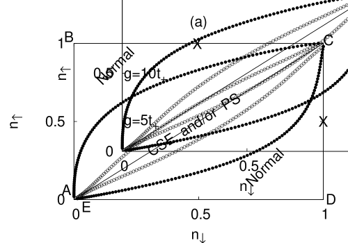
respectively iskin-lattice , and consider two sets of tunneling ratios . The case of is shown in Fig. 1, and the case of is shown in Fig. 2. While corresponds to a one-species (two-hyperfine-state) mixture such as 6Li or 40K, corresponds to a two-species mixture (one-hyperfine-state of each type of atom) such as 6Li and 40K; 6Li and 87Sr; or 40K and 87Sr.
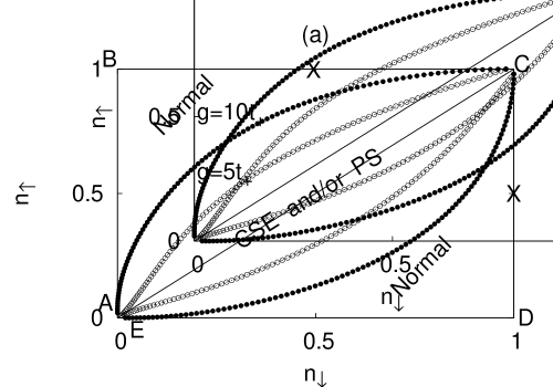

Generally, lines AB (; ) and ED (; ) in Figs. 1 and 2, correspond to normal -type Fermi metal for all interactions, while points B and D correspond to a Fermi-Pauli (band) insulator since there is only one type of fermion in a fully occupied band. Thus, the only option for additional fermions in case B and in case D) is to fill higher energy bands if the optical potential supports it, otherwise the extra fermions are not trapped. For the case where no additional bands are occupied, we label the corresponding phase diagram regions as ‘Inaccessible’ in Figs. 1(b) and 2(b), since either or in these regions. This phase boundary between the ‘Normal’ and the ‘Inaccessible’ phase is given by for , and for .
The population balanced line AC ends at the special point C, where . This point is a Fermi-Pauli (band) insulator for weak attraction since both fermion bands are fully occupied. Furthermore, for very weak attraction, lines BC () and CD () correspond essentially to a fully polarized ferromagnetic metal (or half-metal), where only the type of fermions with filling fraction less than one can move around.
In the phase diagrams shown in Figs. 1 and 2, we indicate the regions of normal (N) phase where , and group together the regions of coexistence of superfluidity and excess fermions (CSE) and/or phase separation (PS), where . When , the phase diagrams are similar to the homogenous case pao ; sheehy ; iskin-mixture ; iskin-mixture2 , and the versus phase diagram is symmetric for equal tunnelings as shown in Fig. 1(b), and is asymmetric for unequal tunnelings having a smaller normal region when the lighter band mass fermions are in excess as shown in Fig. 2(b). Here, we do not discuss separately the CSE and PS regions since they have already been discussed in homogeneous and harmonically trapped systems pao ; sheehy ; iskin-mixture ; iskin-mixture2 , and experimentally observed mit ; rice ; mit-2 ; rice-2 , but we make two remarks.

First, the lattice phase diagram is also different from the homogenous systems’ in relation to the topological quantum phase transitions discussed in Ref. iskin-mixture ; iskin-mixture2 . These phases are characterized by the number of zero-energy surfaces of and such that (I) has no zeros and has only one, (II) has no zeros and has two zeros, and (III) and has no zeros and are always positive corresponding to the limit. The topological phases characterized by the number (I and II) of simply connected zero-energy surfaces of may lie in the stable region of CSE, unlike in the homogeneous case where the topological phase II always lies in the phase separated region for all parameter space iskin-mixture ; iskin-mixture2 .
To understand the topology of the uniform superfluid phase, we define For the s-wave symmetry considered, the zeros of occur at real momenta provided that for , and for . The transition from phase II to I occurs when , indicating a change in topology in the lowest quasiparticle band. The topology is of phase I if , and phase II is possible only when , and therefore phase II (I) always appears in the BCS (BEC) side of the phase diagram. In the particular case when , the topology is of phase I if , and phase II is possible only when .
Notice that, goes below the bottom of particle (hole) band as increases, since the Cooper pairs are formed from particles (holes) when () iskin-prb . This leads to a large and negative (positive) for particle (hole) pairs in the BEC limit, thus leading to a uniform superfluid with topological phase I (II). Therefore, the topology of the entire superfluid phase is expected to be of phase II for . However, when , the boundary between phase II and phase I lies around for and for .
Similar topological phase transitions in nonzero angular momentum superfluids have been discussed previously in the literature in connection with 3He p-wave phases leggett ; volovik-book and cuprate d-wave superconductors duncan , and more recently a connection to ultracold fermions which exhibit p-wave Feshbach resonances was made volovik-pwave ; botelho-pwave ; gurarie-pwave ; skyip-pwave . However, we would like to emphasize that the topological transition discussed here is unique, since it involves a stable s-wave superfluid, and may be observed for the first time in future experiments.
Second, the phase diagram characterized by normal, superfluid (CSE or PS), and insulating regions may be explored experimentally by tuning the ratio , total filling fraction , and population imbalance as done in harmonic traps mit ; rice ; mit-2 ; rice-2 . We would like to emphasize that our saddle point results provide a non-perturbative semi-quantitative description of the normal/superfluid phase boundary for all couplings and tells us that the system is either superfluid or normal , but fails to describe the insulating phases. Thus, first, we analyze Gaussian fluctuations at zero and finite temperatures, and then show that insulating phases emerge from fluctuation effects beyond the saddle point approximation.
IV Gaussian fluctuations
In this section, we follow closely the formalism developed to deal with fluctuations for homogeneous superfluids carlos ; jan ; iskin-mixture ; iskin-mixture2 . We determine the collective modes for Fermi superfluids in optical lattices at zero temperature and the efffective equation of motion near the critical temperature.
IV.1 Gaussian Fluctuations
at Zero Temperature
Next, we analyze the zero temperature Gaussian fluctuations in the BCS and BEC limits for , from which we extract the low frequency and long wavelength collective excitations. For the s-wave symmetry considered, the collective excitation spectrum is determined from the poles of the fluctuation matrix in much the same way as in homogenous systems iskin-mixture2 . Thus, following Ref. iskin-mixture2 , we obtain the condition
| (15) |
where the expansion coefficients and are given in App. A. There are amplitude and phase branches for the collective excitations, but we focus only on the lowest energy Goldstone phase mode with dispersion where
| (16) |
is the speed of sound. First, we discuss analytically the sound velocity in the weak and strong attraction limits, and then calculate numerically the evolution in between these limits.
In the weak attraction (BCS) limit when , the coefficient that couples phase and amplitude fields vanish (), and the phase and amplitude modes are decoupled. We also obtain and where is the number of dimensions. Here, is the density of states and is the Fermi velocity, where is the delta function and is an effective ‘kinetic’ density of states. In addition, we find for the order parameter and for the chemical potential.
The calculation given above leads to which reduces to the Anderson-Bogoliubov relation when . In this limit, the sound velocity can also be written as where Here, is the density of states, and
In the strong attraction (BEC) limit when for and for , the coefficient indicates that the amplitude and phase fields are coupled. We obtain and where we used for the order parameter and for the average chemical potential. Notice that, , where is the binding energy defined by
| (17) |
and is the Hartree energy. Thus, we obtain for the sound velocity, where Notice that, has a dependence in the dilute limit which is consistent with the homogenous result where the sound velocity depends on the square-root of the density. However, saturates to a finite value as increases which is sharp in contrast with the vanishing sound velocity of homogenous systems jan ; iskin-mixture2 .
When (), making the identification that the number of particle (hole) pairs per lattice site is (), we obtain () as the repulsive particle (hole) boson-boson interaction such that the Bogoliubov relation is recovered. Here, we also identified as the mass of the bound pairs to be discussed in Sec. IV.2. Therefore, in both low and high filling fraction limits, we find that .
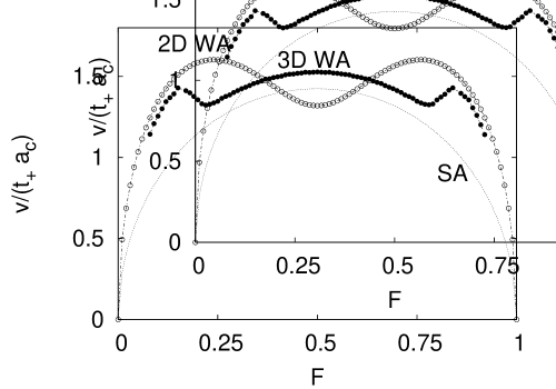
In Fig. 3, we show the sound velocity for two and three dimensional lattices as a function of when and . In the BCS limit shown for , is very different for two and three dimensional lattices due to van Hove singularities present in their density of states sofo ; micnas . However, in the BEC limit shown for , saturates to a finite value, which is identical for both two and three dimensional lattices and reproduces the analytical results discussed above.
Before concluding this section, we discuss the fraction of condensed pairs to understand further the saturation of sound velocity in the BEC limit. In the absence of a population imbalance (), the number of condensed pairs per lattice site is given by leggett-He
| (18) |
where is the ground state pair wave function. At zero temperature, while the number of condensed pairs is very small in comparison to the total number of fermions in the BCS limit, it increases as a function of interaction strength and saturates in the BEC limit to leading to the number of condensed bosons per lattice site as Here, the number of bosons per lattice site is . Therefore, in the dilute limit when , almost all of the bosons are condensed such that , however, in the dense limit when , almost all of the bosons are non-condensed such that . Making the identification that the number of condensed bosons is , we obtain as the repulsive particle (hole) boson-boson interaction such that the Bogoliubov relation is recovered.
Having discussed Gaussian fluctuations at zero temperature, we analyze next Gaussian fluctuations near the critical temperature and derive the time-dependent Ginzburg-Landau (TDGL) functional.
IV.2 Gaussian Fluctuations
Near the Critical Temperature
In this section, we present the results of finite temperature Gaussian fluctuations near the superfluid critical temperature . We define the field to be the fluctuation around the order parameter saddle point value , and use the same procedure as in the homogeneous case carlos ; iskin-mixture2 , to obtain the TDGL functional
| (19) |
in the position and time representation. The expansion coefficients and are given in App. B. Notice that is isotropic for the s-wave interactions considered in this manuscript, where is the Kronecker delta. Next, we discuss analytically the TDGL functional in the weak and strong attraction limits.
In the weak attraction (BCS) limit when , it is difficult to derive analytical expressions in the presence of population imbalance, and thus we limit our discussion only to the limit. In this case, we obtain for the coefficient of the linear term in , for the cofficient of the cubic term, for the coefficent of the operator , and for the coefficient of the operator . Here, represents an effective ‘kinetic’ density of states, and the parameter is the BCS critical temperature where is the Euler’s constant, and is the Zeta function. Notice that is quite small for weak attractions, but increases with growing values of . In addition, notice that the imaginary part of is large, indicating that Cooper pairs have a finite lifetime and that they decay into the continuum of two-particle states.
In the strong attraction (BEC) limit when , we obtain for the coefficient of the linear term in , for the cofficient of the cubic term, for the coefficent of the operator , and for the coefficient of the operator . Here, is the binding energy, () labels the excess (non-excess) type of fermions, and is the number of unpaired fermions per lattice site. Notice that the imaginary part of vanishes in this limit, reflecting the presence of long lived bound states.
Through the rescaling , we obtain the equation of motion for a mixture of bound pairs (molecular bosons) and unpaired (excess) fermions
| (20) | |||||
with boson chemical potential mass and repulsive boson-boson and boson-fermion interactions. Notice that, the repulsion between bound pairs is two times larger than the repulsion between a bound pair and a fermion, reflecting the Pauli exclusion principle. Furthermore, and are strongly repulsive due to the important role played by the Pauli exclusion principle in the lattice iskin-lattice , in contrast to the homogenous case carlos ; pieri ; iskin-mixture ; iskin-mixture2 where and are weakly repulsive.
This procedure also yields , which is the spatial density of unpaired fermions
| (21) |
The critical temperature in the case of zero population imbalance can be obtained directly from the effective boson mass , using the standard BEC condition leading to , which decreases with growing attraction . Here, is the zeta function. Notice that in the lattice case vanishes for unlike the homogeneous case which saturates at , where is the Fermi energy nsr ; carlos . The decrease of with increasing in the BEC regime, combined with the increase of with increasing in the BCS regime leads to a maximum in between as already noted in the literature nsr ; micnas .
Further insight into the differences between the homogeneous and the lattice systems can be gained by comparing the Ginzburg-Landau coherence length which in the vicinity of becomes The prefactor of the coherence length is
| (22) |
and is evaluated at . While is large in the weak attraction limit in comparison to the lattice spacing , is small and phase coherence is lost gradually as increases in the strong attraction limit when . This latter result is in sharp contrast with the homogenous case carlos , where is large compared to interparticle spacing in both BCS and BEC limits, and it has a minimum near carlos . However, depends inversely on the square-root of the density in both homogenous and lattice systems.
Since the boson-boson and boson-fermion interactions are strongly repulsive in the BEC limit (strong attraction regime for fermions) due to the important role played by the Pauli exclusion principle in the lattice iskin-lattice , it is necessary to investigate this further, as discussed next.
V Strong Attraction (Molecular) Limit
In the strong attraction limit, the system can be described by an action containing molecular bosons and excess fermions pieri ; iskin-mixture ; iskin-mixture2 . The existence of an optical lattice produces different physics from the homogeneous case in the strong attraction limit, because of the strong repulsive interaction between molecular bosons and excess fermions iskin-lattice . The main effect of these strong effective interactions is the emergence of insulating phases from the resulting Bose-Fermi mixture of molecular bosons and excess fermions in a lattice.
V.1 Effective Lattice Bose-Fermi Action
In the limit of strong attractions between fermions , we obtain an effective Bose-Fermi lattice action iskin-lattice
| (23) |
where Here, the kinetic part of the excess fermions is
| (24) |
the kinetic part of the molecular bosons is
| (25) |
the interaction between molecular bosons and excess fermions is
| (26) |
and the interaction between two molecular bosons is
| (27) |
The total number of fermions is fixed by the constraint , where is the number of bosons per lattice site. The important parameters of this effective Hamiltonian are the excess fermion transfer energy , the molecular boson transfer energy , the boson-fermion effective repulsion and the boson-boson effective repulsion . Notice that, on-site interactions and become infinite (hard-core) when as a manifestation of the Pauli exclusion principle. In addition, there are weak and repulsive nearest neighbor boson-boson and boson-fermion interactions. These repulsive interactions in optical lattices lead to several insulating phases, depending on fermion filling fractions, as discussed next.
V.2 Emergence of Insulating Phases
When the fermion attraction is sufficiently strong, the lines BC and CD must describe insulators, as molecular bosons and excess fermions are strongly repulsive. In the following analysis, we discuss only two high symmetry cases: (a) ; and (b) and , or and .
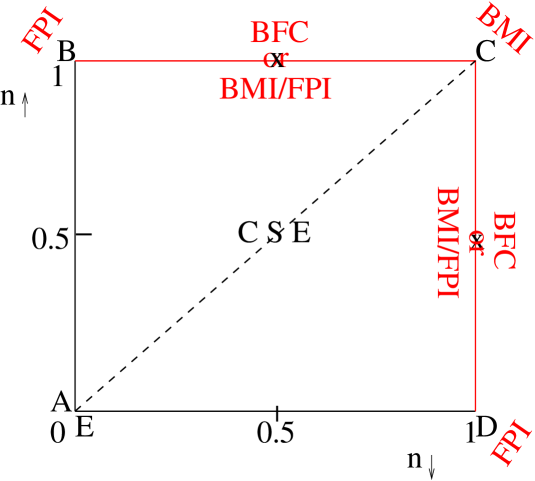
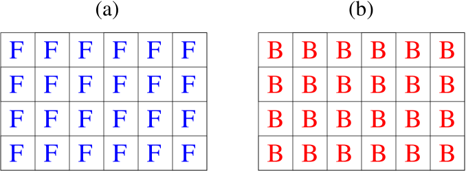
Case (a) is indicated as point C in Figs. 1, 2 and 4 where such that . This symmetry point is a Fermi-Pauli (band) insulator for weak attraction since both fermion bands are fully occupied, and a Bose-Mott Insulator (BMI) in the strong attraction limit. There is exactly one molecular boson (consisting of a pair of and fermions) at each lattice site, which has a strong repulsive on-site interaction with any additional molecular boson due to the Pauli exclusion principle. Notice that this case is very similar to the atomic BMI transition observed with one-species atomic Bose systems bloch-review .
In case (a), reduces to a molecular Bose-Hubbard Hamiltonian with the molecular Bose filling fraction , thus leading to a molecular BMI when beyond a critical value of . A schematic diagram of this phase is shown in Fig. 5(b). The critical value needed to attain the BMI phase can be estimated using the approach of Ref. stoof-2001 leading to , which in terms of the underlying fermion parameters leads to for the critical fermion interaction. This value of is just a lower bound of the superfluid-to-insulator (SI) transition, since is only valid in the limit. Some signatures of this SI transition at have been observed in recent experiments mit-lattice .
We would like to make some remarks on the validity presented above, which intrinsically assumes that the molecular bosons are small in comparison to the lattice spacing. A measure of the ‘smallness’ of these molecular bosons is the average size of the fermion pairs defined (for ) by
| (28) |
where is the ground state pair wave function. While is large in the weak attraction limit in comparison to the lattice spacing , in the strong attraction limit when . These expressions are valid for low and high filling fractions, and , respectively. At , we obtain for and for . Notice that larger values of lead to molecular boson sizes that are smaller than the lattice spacing, thus validating the effective Bose-Fermi description derived above for to values of close to . In the lattice case, the results above suggest that even if the size of the bound pairs decreases as with increasing , the Pauli pressure prohibits two bound pairs or a bound pair and an excess fermion to occupy the same lattice site, in the single-band description discussed here. This indicates that the bound pairs do not loose their fermionic nature and can not be thought as structureless in lattices, which should be contrasted with the homogenous case where bound pairs become structureless with increasing attraction.
Case (b) is indicated as crosses in Figs. 1, 2 and 4 at points or , where the molecular boson filling fraction and the excess fermion filling fraction is . At these high symmetry points, molecular bosons and excess fermions tend to segregate, either producing a domain wall type of phase separation between a molecular Bose-Mott insulator (BMI) region and a Fermi-Pauli insulator (FPI) region or a checkerboard phase of alternating molecular bosons and excess fermions (BFC) depending on the ratio . A schematic diagram of these two phases is shown in Fig. 6.
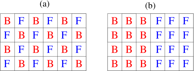
The checkerboard phase shown in Fig 6(a) is favored when . At the current level of approximation, we find that when phase separation is always favored, however when () fermions are in excess the checkerboard phase is favored when . Therefore, phase separation and checkerboard phases are achievable if the tunneling ratio can be controlled experimentally in optical lattices. Notice that this checkerboard phase present in the lattice case is completely absent in homogeneous or harmonically trapped systems pao ; sheehy ; iskin-mixture ; iskin-mixture2 .
Thus, the strong attraction limit in optical lattices brings additional physics not captured at the saddle point, and not present in homogenous or purely harmonically trapped systems. Having discussed the strong attraction (molecular) limit and its possible phases, we comment next on their experimental detection.
VI Detection of Insulating Phases
It may be very difficult to detect all the superfluid and insulating phases proposed in situ, and thus one may have to turn off the optical lattice to perform time-of-flight measurements. The phases proposed here in the molecular limit could be detected either via the measurement of momentum distribution, density-density correlations or density Fourier transform. For instance, the Fermi-Pauli insulator (FPI), Bose-Mott insulator (BMI), Bose-Fermi checkerboard (BFC), and phase separated BMI/FPI do not exhibit phase coherence in their momentum distribution, while the superfluid phase does. Therefore, through the momentum distribution measurements, one should be able to differentiate between superfluid and insulating phases, which has been possible for Bose systems in optical lattices bloch-review . However, in order to detect clearly the different insulating phases, it may also be necessary to explore the Fourier transforms of the densities, or of the density-density correlation functions.
The relevant density-density correlation functions to characterize the insulating phases are which correlates the excess fermions, which correlates the molecular bosons, and which correlates the molecular bosons and excess fermions. Defining the relative and the sum of the coordinates, we can write the correlation functions as where and are . This leads to the Fourier transform , where is the relative and is the sum of the momentums. For a translationally invariant system considered here, it is sufficient to look only to , and define Therefore, for the FPI, BMI and BFC insulating phases, correlation functions have the generic form where and are the locations of and particles.
For instance, in the case of a two-dimensional system, the FPI phase [shown in Fig. 5(a)] has a strong peak in the correlation function at . Similarly, the BMI phase [shown in Fig. 5(b)] has a strong peak in the correlation function at . However, the BFC phase [shown in Fig. 6(a)] has strong peaks in the correlation functions and both at and , while it has strong peaks in the correlation function at .
The insulating FPI, BMI, and BFC phases are modified in the presence of an overall harmonic trapping potential, since the molecular bosons experience the harmonic potential and the excess fermions of type experience a different harmonic potential Provided that the harmonic potentials are not too strong, the characteristic peak locations of the correlation functions remain essentially the same, but additional broadening due to the inhomogeneous nature of the trapping potential occurs. However, when the harmonic potentials are sufficiently large, important modifications of these phases are present, including the emergence of complex shell structures.
Lastly, the BMI/FPI phase separated state is strongly modified even in the presence of weak trapping potentials. The single domain wall density structure [shown in Fig. 6(b)] turns into a new density profile with a region where the bosons tend to stay at the center of the trapping potential due in part to their tighter confinement, and the excess fermions are pushed out of the center by the strong Bose-Fermi repulsion. The fermions then surround the bosons, and standard in situ radio-frequency measurements can detect the existence of the BMI/FPI phase separated state, as done recently with population imbalanced fermion mixtures mit ; rice ; mit-2 ; rice-2 .
Having commented briefly on the experimental detection of the superfluid and insulating phases, we present our conclusions next.
VII Conclusions
Using an attractive Fermi-Hubbard Hamiltonian to describe mixtures of one- or two-species of atoms in optical lattices, we obtained the ground state phase diagram of Fermi-Fermi mixtures containing normal, phase-separated and coexisting superfluid/excess fermions, and insulating regions. We discussed the cases of balanced and imbalanced populations of Fermi-Fermi mixtures such as 6Li or 40K only; and mixtures of 6Li and 40K; 6Li and 87Sr; or 40K and 87Sr. We showed that population imbalanced Fermi-Fermi mixtures reduce to strongly interacting (repulsive) Bose-Fermi mixtures in the molecular limit, in sharp contrast to homogenous systems where the resulting Bose-Fermi mixtures are weakly interacting. This result is a direct manifestation of the Pauli exclusion principle in the lattice case, since each Bose molecule consists of two fermions, and more than one identical fermion on the same lattice site is not allowed, within a single-band description. This effect together with the Hartree energy shift lead to a filling dependent condensate fraction and to sound velocities which do not approach zero, in contrast to the homogenous case.
Furthermore, we showed that several insulating phases appear in the strong attraction limit depending on filling fraction and population imbalance. For instance, we found a molecular Bose-Mott insulator (superfluid) when the molecular filling fraction is equal to (less than) one for a population balanced system where the fermion filling fractions are identical. When the filling fraction of one type of fermion is one and the filling fraction of the other is one-half (corresponding to molecular boson and excess fermion filling fractions of one-half), we also found either a phase-separated state consisting of a Fermi-Pauli insulator (FPI) of the excess fermions and a molecular Bose-Mott insulator (BMI) or a Bose-Fermi checkerboard (BFC) phase depending on the tunneling anisotropy ratio.
All of these additional phases and the possibility of observing more exotic superfluid phases in optical lattices with p-wave order parameters iskin-prb make the physics of Fermi-Fermi mixtures much richer than those of atomic bosons or Bose-Fermi mixtures in optical lattices, and of harmonically trapped fermions. Lastly, the molecular BMI phase discussed here has been preliminarily observed in a very recent experiment mit-lattice , opening up the experimental exploration of the rich phase diagram of fermion mixtures in optical lattices in the near future.
We thank National Science Foundation (DMR-0709584) for support.
Appendix A Expansion Coefficients at Zero Temperature
In this Appendix, we perform a small and expansion of the effective action at zero temperature () iskin-mixture2 . In the amplitude-phase basis, we obtain the expansion coefficients necessary to calculate the collective modes, as discussed in Section IV.1. We calculate the coefficients only for the case of s-wave pairing with zero population imbalance , as extra care is needed when due to Landau damping. In the long-wavelength , and low-frequency limits the condition is used.
The coefficients necessary to obtain the diagonal amplitude-amplitude matrix element are
| (29) |
corresponding to the term,
| (30) | |||||
corresponding to the term, and
| (31) |
corresponding to the term.
The coefficients necessary to obtain the diagonal phase-phase matrix element are
| (32) | |||||
corresponding to the term, and
| (33) |
corresponding to the term.
The coefficient necessary to obtain the off-diagonal matrix element is
| (34) |
corresponding to the term. These coefficients can be evaluated analytically in the BCS and BEC limits, and are given in Sec. IV.1.
Appendix B Expansion Coefficients Near the Critical Temperature
In this Appendix, we derive the coefficients and of the time dependent Ginzburg-Landau theory described in Section IV.2. We perform a small and expansion of the effective action near the critical temperature (), where we assume that the fluctuation field is a slowly varying function of position and time iskin-mixture2 .
The zeroth order coefficient is given by
| (35) |
where and
The second order coefficient is given by
| (36) | |||||
where and Here, is the Kronecker delta.
The fourth order coefficient is given by
| (37) |
The time-dependent coefficient has real and imaginary parts, and for the s-wave case is given by
| (38) |
where is the delta function. These coefficients can be evaluated analytically in the BCS and BEC limits, and are given in Sec. IV.2.
References
- (1) M. W. Zwierlein, A. Schirotzek, C. H. Schunck and W. Ketterle, Science 311, 492 (2006).
- (2) G. B. Partridge, W. Lui, R. I. Kamar, Y. Liao, and R. G. Hulet, Science 311, 503 (2006).
- (3) Y. Shin, M. W. Zwierlein, C. H. Schunck, A. Schirotzek, W. Ketterle, Phys. Rev. Lett. 97, 030401 (2006).
- (4) G. B. Partridge, W. Li, Y. A. Liao, R. G. Hulet, M. Haque, H. T. C. Stoof, Phys. Rev. Lett. 97, 190407 (2006).
- (5) A. J. Leggett, in Modern Trends in the Theory of Condensed Matter, edited by A. Peralski and R. Przystawa, Springer-Verlag, Berlin (1980).
- (6) P. Nozieres and S. Schmitt-Rink, J. Low. Temp. Phys. 59, 195 (1985).
- (7) C. A. R. Sá de Melo, M. Randeria, and J. R. Engelbrecht, Phys. Rev. Lett. 71, 3202 (1993).
- (8) J. R. Engelbrecht, M. Randeria, and C. A. R. Sá de Melo, Phys. Rev. B 55, 15153 (1997).
- (9) P. F. Bedaque, H. Caldas, and G. Rupak, Phys. Rev. Lett. 91, 247002 (2003).
- (10) C. H. Pao, S.-T. Wu, and S. K. Yip, Phys. Rev. B 73, 132506 (2006); and also see cond-mat/0608501 (2006).
- (11) D. E. Sheehy and L. Radzihovsky, Phys. Rev. Lett. 96, 060401 (2006).
- (12) J. K. Chin, D. E. Miller, Y. Liu, C. Stan, W. Setiawan, C. Sanner, K. Xu, and W. Ketterle, Nature 443, 961 (2006).
- (13) G. Modugno, M. Modugno, F. Riboli, G. Roati, and M. Inguscio, Phys. Rev. Lett. 89, 190404 (2002).
- (14) G. Modugno, F. Ferlaino, R. Heidemann, G. Roati, and M. Inguscio, Phys. Rev. A 68, 011601(R) (2003).
- (15) M. Köhl, H. Moritz, T. Stöferle, K. Günter, and T. Esslinger, Phys. Rev. Lett. 94, 080403 (2005).
- (16) T. Stöferle, H. Moritz, K. Günter, M. Köhl, and T. Esslinger, Phys. Rev. Lett. 96, 030401 (2006).
- (17) S. Ospelkaus, C. Ospelkaus, L. Humbert, K. Sengstock, and K. Bongs, Phys. Rev. Lett. 97, 120403 (2006).
- (18) J. Kinnunen, L. M. Jensen, and P. Torma, Phys. Rev. Lett. 96, 110403 (2006).
- (19) P. Pieri and G. C. Strinati, Phys. Rev. Lett 96, 150404 (2006).
- (20) W. Yi and L. M. Duan, Phys. Rev. A 73, 031604 (2006).
- (21) T. N. De Silva and E. J. Mueller, Phys. Rev. A 73, 051602(R) (2006).
- (22) M. Haque and H. T. C. Stoof, Phys. Rev. A 74, 011602 (2006).
- (23) M. Iskin and C. A. R. Sá de Melo, Phys. Rev. Lett. 97, 100404 (2006).
- (24) C. Lobo, A. Recati, S. Giorgini, and S. Stringari, Phys. Rev. Lett. 97, 200403 (2006).
- (25) X.-J. Liu, H. Hu, and P. D. Drummond, Phys. Rev. A 75, 023614 (2007).
- (26) T. Mizushima, M. Ichioka, K. Machida, J. Phys. Soc. Jpn. 76, 104006 (2007).
- (27) M. M. Parish, F. M. Marchetti, A. Lamacraft, B. D. Simons, Phys. Rev. Lett. 98, 160402 (2007).
- (28) M. Iskin and C. A. R. Sá de Melo, Phys. Rev. A 76, 013601 (2007); and also see arXiv:07094424 (2007).
- (29) I. Bloch, Nature Physics 1, 23-30 (2005).
- (30) R. Micnas, J. Ranninger, and S. Robaskiewicz, Rev. Mod. Phys. 62, 113 (1990).
- (31) M. Iskin and C. A. R. Sá de Melo, Phys. Rev. B 72, 224513 (2005); and also see arXiv:cond-mat/0502148 (2005).
- (32) W. V. Liu, F. Wilczek, and P. Zoller, Phys. Rev. A 70, 033603 (2004).
- (33) T. Koponen, T. Paananen, J.-P. Martikainen, and P. Törmä, Phys. Rev. Lett. 99, 120403 (2007).
- (34) Y. Chen, Z. D. Wang, F. C. Zhang, and C. S. Ting, arXiv:0710.5484 (2007).
- (35) M. Iskin and C. A. R. Sá de Melo, Phys. Rev. Lett. 99, 080403 (2007).
- (36) M. Taglieber, A.-C. Voigt, T. Aoki, T. W. Hänsch, and K. Dieckmann, arXiv:0710.2779 (2007).
- (37) E. Wille, F. M. Spiegelhalder, G. Kerner, D. Naik, A. Trenkwalder, G. Hendl, F. Schreck, R. Grimm, T. G. Tiecke, J. T. M. Walraven, S. J. J. M. F. Kokkelmans, E. Tiesinga, and P. S. Julienne, arXiv:0711.2916 (2007).
- (38) G. H. Wannier, Phys. Rev. 52, 191 (1937).
- (39) A. Koetsier, D. B. M. Dickerscheid, and H. T. C. Stoof, Phys. Rev. A 74, 033621 (2006).
- (40) G. E. Volovik, Exotic properties of superfluid 3He, (World Scientific, Singapore, 1992).
- (41) R. D. Duncan and C. A. R. Sá de Melo, Phys. Rev B 62, 9675 (2000); and also see L. S. Borkowski and C. A. R. Sá de Melo, arXiv:cond-mat/9810370 (1998).
- (42) F. R. Klinkhamer and G. E. Volovik, Pisma Zh. Eksp. Teor. Fiz. 80, 389 (2004); JETP Lett. 80, 343 (2004).
- (43) S. S. Botelho and C. A. R. Sá de Melo, J. Low Temp. Phys. 140, 409 (2005); and also see arXiv:cond-mat/0409357 (2004).
- (44) V. Gurarie, L. Radzihovsky, and A. V. Andreev, Phys. Rev. Lett. 94, 230403 (2005).
- (45) C.-H. Cheng and S.-K. Yip, Phys. Rev. Lett. 95, 070404 (2005).
- (46) J. O. Sofo, C. A. Balseiro, and H. E. Castillo, Phys. Rev. B 45, 9860 (1992).
- (47) D. van Oosten, P. van der Straten, and H. T. C. Stoof, Phys. Rev. A 63, 053601 (2001).
- (48) A. J. Leggett, Rev. Mod. Phys. 47, 331 (1975).