Eikonal zeros in the momentum transfer space from proton-proton scattering: An empirical analysis

Abstract

By means of improved empirical fits to the differential cross section data on $pp$ elastic scattering at $19.4\leq\sqrt{s}\leq 62.5$ GeV and making use of a semi-analytical method, we determine the eikonal in the momentum transfer space (the inverse scattering problem). This method allows for the propagation of the uncertainties from the fit parameters up to the extracted eikonal, providing statistical evidence that the imaginary part of the eikonal (real part of the opacity function) presents a zero (change of signal) in the momentum space, at $q^{2}\approx 7\pm 1$ GeV². We discuss the implication of this change of signal in the phenomenological context, showing that eikonal models with one zero provide good descriptions of the differential cross sections in the full momentum transfer range, but that is not the case for models without zero. Empirical connections between the extracted eikonal and results from a recent global analysis on the proton electric form factor are also discussed, in particular the Wu-Yang conjecture. In addition, we present a critical review on the $pp$ differential cross section data presently available at high energies.

Contents

1

Introduction

2

Eikonal representation and the inverse scattering problem

3

Critical discussion on $pp$ differential cross section data at high energies

3.1 Data at 23.5 $\leq\sqrt{s}\leq$ 62.5 GeV

3.2 Data at 19.4 and 27.4 GeV

$3.2.1$ $\sqrt{s}$ = 19.4 GeV

$3.2.2$ $\sqrt{s}$ = 27.4 GeV

3.3 Discussion on data at large momentum transfers

$3.3.1$ References and data

$3.3.2$ Dependence on the energy

4

Improvements in the previous analysis and fit results

4.1 Data ensembles and energy independence

4.2 Parametrization

4.3 Confidence intervals for uncertainties

4.4 Fit results

5

Eikonal in the momentum transfer space

5.1 Semi-analytical method

5.2 Eikonal zeros

6

Phenomenological implication of the eikonal zero

6.1 Eikonal and scattering amplitude

6.2 Some representative eikonal models

$6.2.1$ Models without eikonal zero

$\bullet$ Chou-Yang model

$\bullet$ QCD-inspired models

$6.2.2$ Hybrid model

$6.2.3$ Models with eikonal zero

$\bullet$ Bourrely-Soffer-Wu model

$\bullet$ A multiple diffraction model

$6.2.4$ Discussion

$\bullet$ General aspects

$\bullet$ Quantitative aspects

$\bullet$ Empirical parametrization for the eikonal

6.3 Hadronic and electromagnetic form factors

$6.3.1$ Rosenbluth and polarization transfer results

$6.3.2$ The Proton electric form factor

7

Summary and final remarks

1 Introduction

Quantum Chromodynamics (QCD) is very successful in describing hadronic scattering involving very large momentum transfers gelis . However, that is not the case for soft diffractive processes (large distance phenomena), in particular the simplest process: high-energy elastic hadron scattering. The point is that perturbative techniques can not be applied and presently, non-perturbative approaches can not describe scattering states without strong model assumptions pred ; donna . At this stage phenomenology is an important approach and among the wide variety of models, the eikonal picture plays a central role due to its connection with unitarity pred .

Alongside phenomenological models, empirical analyses, aimed to extract model-independent information from the experimental data (the inverse scattering problem), also constitute important strategy that can contribute with the establishment of novel theoretical calculational schemes. In an unitarized context this approach is characterized by model-independent extraction of the eikonal from empirical fits to the differential cross section data, mainly on proton-proton ($pp$) and antiproton-proton ($\bar{p}p$) scattering (highest energies reached in accelerator experiments). However, one of the main problems with this kind of analysis is the very limited interval of the momentum transfer with available data, in general below 6 GeV². This means that, from the statistical point of view, all the extrapolated curves from the fits must be taken into account, which introduces large uncertainties in the extracted information.

In references cmm ; cm this problem was addressed through a detailed analysis of the experimental data in the region of large momentum transfer and that allowed the extraction to be made of the eikonal on statistical grounds. The main result, from the analysis of $pp$ elastic scattering at $19.4\leq\sqrt{s}\leq 62.5$, concerned the evidence of eikonal zeros (change of sign) in the momentum transfer space and that the position of the zero decreases as the energy increases cmm . As discussed in that paper, this kind of model independent information in the momentum space is very important in the construction and selection of phenomenological approaches, mainly in the case of diffraction models, since the eikonal, in the momentum transfer space, is expected to be connected with hadronic form factors and elementary cross sections.

In this work, we introduce two main improvements in this previous analysis, which are related with the ensemble of the selected data and the structure of the parametrization. We still obtain statistical evidence for the zeros, but different from cmm , it can not be inferred that the position of the zero decreases as the energy increases (some preliminary results on this feature appear in amm ). In order to explain some subtleties involved in the analysis, we present a novel critical review and discussions on the $pp$ differential cross section data presently available. That may be very opportune since presently a great development is expected of the area with the next $pp$ experiments at 200 GeV (BNL RHIC) pp2pp and 14 TeV (CERN LHC) totem . In addition, we discuss in some detail the implication of the eikonal zero in the phenomenological context, introducting a novel analytical parametrization for the extracted eikonal. Connections between the empirical result for the eikonal and recent data on the proton electric form factor are also presented and discussed, in particular the Wu-Yang conjecture.

The manuscript is organized as follows. In Sect. 2 we recall the main formulas connecting the experimental data and the eikonal (the inverse scattering problem). In Sect. 3 we present a critical review on the experimental data presently available from elastic $pp$ scattering. In Sect. 4 we discuss the improvements introduced in the previous analysis and present the new fit results. In Sect. 5 we treat the determination of the eikonal in the momentum transfer space and in Sect. 6 we discuss the implication of the eikonal zeros in the phenomenological context, as well as connections between the extracted eikonal, models and the proton electric form factor. The conclusions and some final remarks are the contents of Sect. 7.

2 Eikonal representation and the inverse scattering problem

In the eikonal representation, the elastic scattering amplitude can be expressed by pred

$$F(s,q)=\mathrm{i}\int_{0}^{\infty}b\mathrm{d}bJ_{0}(qb)\{1-\mathrm{e}^{\mathrm{i}\chi(s,b)}\},$$ (1)

where $s$ is the center-of-mass energy squared, $q^{2}=-t$ the four-momentum transfer squared, $b$ the impact parameter and $\chi(s,b)$ the eikonal function in the impact parameter space (azimuthal symmetry assumed). It is also useful to define the Profile function (the inverse transform of the amplitude) in terms of the eikonal:

$$\Gamma(s,b)=1-\mathrm{e}^{\mathrm{i}\chi(s,b)}.$$ (2)

With these definitions the complex eikonal corresponds to the continuum complex phase shift, in the limit of high energies and the semi-classical approximation: $\chi(s,b)=2\delta(s,b)$; that is also the normalization in the Fraunhofer regime pred .

In the theoretical context, eikonal models are characterized by different phenomenological choices for the eikonal function in the momentum transfer space:

$$\tilde{\chi}(s,q)=\int_{0}^{\infty}b\mathrm{d}bJ_{0}(qb)\chi(s,b).$$ (3)

On the other hand, the inverse scattering problem deals with the empirical determination, or extraction, of the eikonal from the experimental data on the differential cross section

$$\frac{\mathrm{d}\sigma}{\mathrm{d}q^{2}}=\pi|F(s,q)|^{2},$$ (4)

the total cross section (optical theorem)

$$\sigma_{\mathrm{tot}}(s)=4\pi\mathrm{Im}\ F(s,q=0),$$ (5)

and the parameter $\rho$, defined as the ratio of the real to the imaginary part of the forward amplitude,

$$\rho(s)=\frac{\mathrm{Re}\ F(s,q=0)}{\mathrm{Im}\ F(s,q=0)}.$$ (6)

Formally, from a model independent parametrization for the scattering amplitude and fits to the differential cross section data, one can extract the profile function

$$\Gamma(s,b)=-\mathrm{i}\int_{0}^{\infty}q\mathrm{d}qJ_{0}(qb)F(s,q),$$ (7)

the eikonal in the impact parameter space,

$$\chi(s,b)=-\mathrm{i}\ln\left[1-\Gamma(s,b)\right],$$ (8)

and then, under some conditions, the eikonal in the momentum transfer space through Eq. (3). The possibility to extract $\tilde{\chi}(s,q)$ is very important if we look for possible connections with quantum field theory since elementary (partonic) cross sections are expressed in the momentum transfer space as well as form factors of the nucleons.

However, as already commented on in our introduction, we stress that a drawback of the above inverse scattering is the fact that the differential cross section data available cover only limited regions in terms of the momentum transfer, which in general is small, as referred and discussed in what follows. This can be contrasted with the fact that, in order to extract the eikonal, all the Fourier-Bessel transforms must be performed in the interval $0\rightarrow\infty$. Therefore, data at large values of the momentum transfer play a central role in this kind of analysis and for that reason we first discuss in the next section the experimental data presently available and some subtleties involved in the selection, normalization and interpretation of the data sets. A detailed analysis of data at small $q^{2}$ is discussed in cudell and extended in clm .

3 Critical discussion on $pp$ differential cross section data at high energies

In Ref. cmm it has been shown that the lack of sufficient experimental information on $\bar{p}p$ elastic differential cross sections does not allow to perform the kind of analysis we are interested in. For that reason we shall treat here only $pp$ elastic scattering at the highest energies, namely $\sqrt{s}$ above $\approx$ 19 GeV.

The inputs of our analysis concern the experimental data on differential cross section, total cross section, the $\rho$ parameter and the corresponding optical point:

$$\left.\frac{\mathrm{d}\sigma}{\mathrm{d}q^{2}}\right|_{q^{2}=0}=\frac{\sigma_{\mathrm{tot}}^{2}(1+\rho^{2})}{16\pi},$$ (9)

where $\rho(s)$ and $\sigma_{\mathrm{tot}}(s)$ are the experimental values at each energy. Since we are interested only in the hadronic interaction, the selected differential cross section data cover the region above the Coulomb-nuclear interference, namely $q^{2}>$ 0.01 GeV². In what follows we discuss the sets of data at 7 different energies, divided in the two groups 23.5 $\leq\sqrt{s}\leq$ 62.5 GeV (5 sets) and $\sqrt{s}$ = 19.4 and 27.4 GeV.

3.1 Data at 23.5 $\leq\sqrt{s}\leq$ 62.5 GeV

The five data sets at $\sqrt{s}$ = 23.5, 30.7, 44.7, 52.8 and 62.5 GeV were obtained at the CERN Intersecting Storage Ring (ISR) in the seventies and still represent the largest and highest energy range of available data on $pp$ scattering (the recent experiment at RHIC by the $pp2pp$ Collaboration measured only the slope parameter at $\sqrt{s}$ = 200 GeV pp2ppslope ). The data on $\sigma_{\mathrm{tot}}$, $\rho$ and $\mathrm{d}\sigma/\mathrm{d}q^{2}$ were compiled and analyzed by Amaldi and Schubert leading to the most coherent set of data on $pp$ scattering. Detailed information on this analysis can be found in as ; here we only recall some relevant aspects to our discussion.

Optical points. The numerical values for the total cross sections, correspond to the average of 3 experiments, performed in each of the above energies; the $\rho$ data comes from 2 experiments, one at 23.5 GeV and the other in the region 30.7 - 62.5 GeV. These numerical values are displayed in Table 1, together with the corresponding optical points (and references for the $\rho$ data).

Table 1: Forward data ($\sigma_{\mathrm{tot}}$ and $\rho$) and optical points from $pp$ scattering used in this analysis.

$\sqrt{s}$	$\sigma_{\mathrm{tot}}$	$\rho$	$\mathrm{d}\sigma/\mathrm{d}q^{2}|_{q^{2}=0}$
(GeV)	(mb)		(mbGeV-2)
19.4	38.98 $\pm$ 0.04 car	0.019 $\pm$ 0.016 faj	77.66 $\pm$ 0.02
23.5	38.94 $\pm$ 0.17 as	0.02 $\pm$ 0.05 a1	77.5 $\pm$ 0.7 as
30.7	40.14 $\pm$ 0.17 as	0.042 $\pm$ 0.011 a2	82.5 $\pm$ 0.7 as
44.7	41.79 $\pm$ 0.16 as	0.0620 $\pm$ 0.011 a2	89.6 $\pm$ 0.7 as
52.8	42.67 $\pm$ 0.19 as	0.078 $\pm$ 0.010 a2	93.6 $\pm$ 0.8 as
62.5	43.32 $\pm$ 0.23 as	0.095 $\pm$ 0.011 a2	96.8 $\pm$ 1.1 as

Data beyond the forward direction ($q^{2}>$ 0.01 GeV²). The data in the region of small momentum transfer were normalized to the optical point and above this region different data sets were normalized relative to each other, taking into account both the statistical and systematic errors (see as for details). The final result of this coherent and accurate analysis of the differential cross sections were published in the numerical tables of the series Landolt-Börnstein (LB) lb , from which we extracted our data sets. They are reproduced in Fig. 1, together with the optical points (Table 1). As we can see, the largest set with available data correspond to $\sqrt{s}$ = 52.8 GeV, with $q_{\mathrm{max}}^{2}$ = 9.75 GeV². Except for the data at 44.7 GeV all the other sets cover the region nearly below 6 GeV².

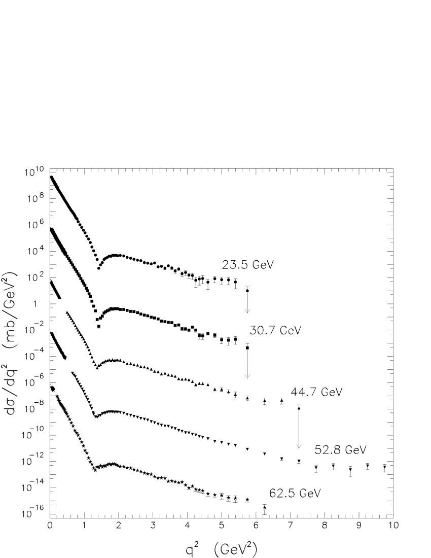
Figure 1: Proton-proton differential cross section data at the ISR energy region from Landolt Börnstein tables lb and optical points from Table 1. Data were multiplied by factors of $10^{\pm 4}$.

3.2 Data at $\sqrt{s}$ = 19.4 and 27.4 GeV

These sets correspond to the largest values of the momentum transfer with available data, namely $q_{\mathrm{max}}^{2}$ = 11.9 GeV² ($\sqrt{s}$ = 19.4 GeV) and $q_{\mathrm{max}}^{2}$ = 14.2 GeV² ($\sqrt{s}$ = 27.4 GeV). For that reason they play a fundamental role in our analysis. In especial, as we shall discuss, data at 27.4 GeV are crucial for the statistical evidence of the eikonal zero and data at 19.4 GeV is extremely important for giving information on the energy dependence of the position of the zero.

These data were obtained in the seventies-eighties at the Fermi National Accelerator Laboratory (Fermilab) and at the CERN Super Proton Synchrotron (SPS). Some of these data sets were then published or made available from the authors in a preliminary form. We call attention to this fact because comparisons and interpretation may occur that are not consistent with what can be inferred from the final published results. In this section we first list and summarize our selection of the experimental data and then discuss the information that can be extracted from these ensembles.

3.2.1 $\sqrt{s}$ = 19.4 GeV

Optical point. We evaluate the optical point, Eq. (9), with the values of the total cross section obtained by Carrol et al. car and the $\rho$ parameter by Fajardo et al. faj (Table 1). Both experiments were performed at the Fermilab with beam momentum $p_{\mathrm{lab}}$ = 200 GeV ($\sqrt{s}$ = 19.42 GeV).

Data beyond the forward direction. We made use of the following data sets:

0.075 $\leq q^{2}\leq$ 3.25 GeV². Final data published by Akerlof et al. akerlof and obtained at the Fermilab with $p_{\mathrm{lab}}$ = 200 GeV. The errors are statistical and the absolute normalization uncertainty is 7 %.

5.0 $\leq q^{2}\leq$ 11.9 GeV². Final results from Faissler et al. faissler , obtained at the Fermilab with $p_{\mathrm{lab}}$ = 201 GeV ($\sqrt{s}$ = 19.47 GeV). The errors are statistical and overall normalization error is 15 %.

0.6125 $\leq q^{2}\leq$ 3.90 GeV². Data obtained by Fidecaro et al. fidecaro , at the CERN-SPS with $p_{\mathrm{lab}}$ = 200 GeV. The $q^{2}$ values correspond to the central values of the bins from [0.600 - 0.625] to [3.8 - 4.0]. The data are normalized fidecaro and the errors are statistical.

0.95 $\leq q^{2}\leq$ 8.15 GeV². Final results from Rubinstein et al. rubinstein , obtained at the Fermilab with $p_{\mathrm{lab}}$ = 200 GeV. The errors are statistical and systematic uncertainties in overall normalization are 15 %. The points at $q^{2}$ = 6.55 and 8.15 GeV² have a statistical error of 100 %.

3.2.2 $\sqrt{s}=27.4$ GeV

The data cover the region 5.5 $\leq q^{2}\leq$ 14.2 GeV² and we have used the final results from Faissler et al. faissler , obtained at the Fermilab with $p_{\mathrm{lab}}$ = 400 GeV ($\sqrt{s}$ = 27.45 GeV). The errors are statistical and overall normalization error is 15 %.

All these data at 19.4 and 27.4 GeV are displayed in Fig. 2 with the statistical errors. The intervals in the momentum transfer of all data referred to above, $19.4\leq\sqrt{s}\leq 62.5$ GeV, are summarized in Table 2.

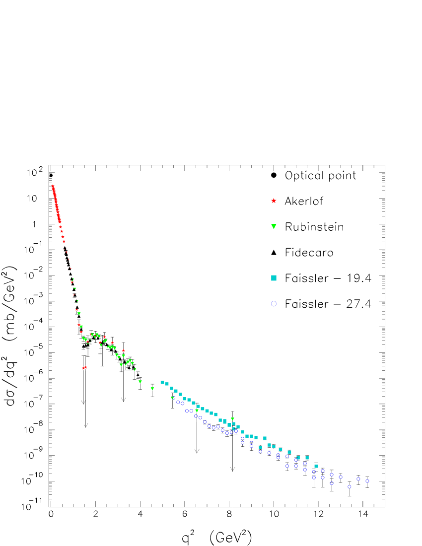
Figure 2: Differential cross section data at $\sqrt{s}$ = 19.4 GeV and 27.4 GeV used in this analysis.

Table 2: Intervals in the momentum transfer for the differential cross section data at $q^{2}>0.01$ GeV² (above the Coulomb-nuclear interference region), number of points used in this analysis and references for the tables.

$\sqrt{s}$ (GeV)	$q^{2}$ interval (GeV2)	Number of points	References
19.4 (Fermilab and CERN-SPS)	0.075 - 11.9	156	akerlof ; faissler ; fidecaro ; rubinstein
23.5 (CERN-ISR)	0.042 - 5.75	172	lb
27.4 (Fermilab)	5.5 - 14.2	39	faissler
30.7 (CERN-ISR)	0.016 - 5.75	211	lb
44.7 (CERN-ISR)	0.01026 - 7.25	246	lb
52.8 (CERN-ISR)	0.01058 - 9.75	244	lb
62.5 (CERN-ISR)	0.01074 - 6.25	163	lb

3.3 Discussion on data at large momentum transfers

We now focus the discussion on the experimental data available in the region of large momentum transfer, which, as already noted, play a central role in the global information that can be extracted from the fit procedure (uncertainty region and error propagation). We first call attention to some differences appearing in the published data and then discuss the dependence on the energy of data above $q^{2}$ = 3 - 4 GeV² in the region of interest 19 - 63 GeV (Figures 1 and 2). To clarify some points we shall follow a nearly chronological order.

3.3.1 References and data

As we have seen, the final data from the CERN-ISR at 23.5 $\leq\sqrt{s}\leq$ 62.5 GeV, compiled and normalized by Amaldi and Schubert, were published in LB tables in 1980. Concerning this ensemble it should be noted that final data from experiments, at large momentum transfer, were previously published by Nagy et al. in 1979 nagy , covering the region above 0.825 GeV² ($\sqrt{s}$ = 23.5, 52.8. 62.5) and above 0.975 GeV² ($\sqrt{s}$ = 30.7, 44.7). The point here is that although the authors refer to final results, the numerical values appearing in the LB tables are about 3 % higher than those by Nagy et al.. This difference may be due to the normalization process by Amaldi and Schubert, referred to in Sect. 3.1.

The data at 19.4 and 27.4 also appear in the LB tables and in this case we first note that: 1) these data did not take part in the analysis by Amaldi and Schubert (only ISR data) being, therefore, not normalized; 2) some numerical values appearing in the tables are preliminary and do not correspond to final published results, as discussed in what follows; 3) other data at 19.4 were published after 1980 fidecaro ; rubinstein (Sect. 3.2).

At 19.4 GeV, the data appearing in the LB tables in the region 0.075 $\leq q^{2}\leq$ 3.25 GeV² are exactly the same as those published by Akerlof et al. in 1976 akerlof . However, data at this energy in the region 5.5 $\leq q^{2}\leq$ 11.9 GeV² and those at 27.4 GeV and 5.5 $\leq q^{2}\leq$ 14.2 GeV² do not correspond to the final values published by Faissler et al. in 1981 faissler . The differences, in the case of data at 27.4 GeV, are illustrated in Fig. 3, where we see that although the general trend of both sets are similar, the corrections are different in different regions of the momentum transfer (the geometries of the experiment at mid and high $q^{2}$ values faissler ). Moreover, the preliminary set appearing in the LB tables has 30 data points and the final set by Faissler et al. presents 39 data. We shall return to this point when discussing the improvements in our previous analysis (Sect. 4.1).

Figure 3: Differential cross section data on $pp$ scattering at 27.4 GeV from the Landolt-Börnstein tables lb (black circles) and from Faissler et al. faissler (white circles). The uncertainties correspond to the statistical errors only.

3.3.2 Dependence on the energy

It has been argued that the data on $pp$ scattering at large momentum transfers ($q^{2}>$ 3 - 4 GeV²) and energies above $\sqrt{s}\sim$ 19 GeV have a small dependence on the energy. That represents an important aspect because, if this dependence can be neglected, the information at the largest values of the momentum transfer (for example, data at 27.4 GeV) can be added to sets at nearby energies leading to a drastic reduction of the uncertainty regions in fit procedures. In fact that was the strategy in previous analysis that allowed the statistical evidence to be inferred for the eikonal zeros cmm ; cm . However, the exact value of the energy and momentum transfer above which this dependence can be neglected is not clear in the literature. In what follows, we first recall some previous results, comparisons and arguments and then present a quantitative test which allow to infer numerical limits or bounds for the independence on the energy.

In this respect the main ensemble is obviously the data at 19.4 and 27.4, published by Faissler et al. in 1981, since they cover the region up to 11.9 and 14.2 GeV², respectively. One important result of this measurement was that the data showed no sign of a second dip at large momentum transfer (this dip was previously suggested by the ISR data at 52.8 GeV and $q^{2}\sim$ 8 - 9 GeV² - Fig. 1). Faissler et al. indicate that the ratio of the differential cross section data at 19.4 and 27.4 GeV, for the same $q^{2}$ and interval analyzed, is about 2.3. This difference can be seen in Fig. 2, indicating therefore a reasonable energy dependence. The authors also present comparison of the data at 27.4 GeV and those at 52.8 GeV (ISR). For the ISR data they quote the paper published by De Kerret et al. in 1977 dekerret , where no table is available, only a plot of the data; there is also no reference to the final values published by Nagy et al. in 1979 nagy . According to Faissler et al., comparison of data at 27.4 GeV with those preliminary results at 52.8 GeV indicated a ratio of 1.5 $\pm$ 0.3, after taking into account the normalization errors quoted in both experiments. The authors conclude that the energy dependence is significantly less for $\sqrt{s}>$ 27.4 GeV than it is for $\sqrt{s}<$ 27.4 GeV, referring to a small energy dependence beyond 27.4 GeV for 5 $<q^{2}<$ 8 GeV² faissler .

Another aspect discussed by these authors concerns the value of the slope of the differential cross section at large momentum transfers. In particular, they show that the data at 27.4 GeV follow a power fit of the form $(q^{2})^{-\lambda}$ with $\lambda=$ 8.45 $\pm$ 0.1 and $\chi^{2}$ = 33 for 28 degrees of freedom faissler . This result was interpreted as consistent with the QCD multiple-gluon-exchange calculation by Donnachie and Landshoff, which predicts $\lambda$ = 8 land .

In order to get some quantitative and detailed information on the energy dependence of the data at large momentum transfer, $q^{2}>$ 3 - 4 GeV², and in the energy region of interest (19 - 63 GeV), we have performed several tests with our selected data (Sect. 3.1 and 3.2), taking into account only the statistical errors. We consider the following parametrization

$$\frac{\mathrm{d}\sigma}{\mathrm{d}q^{2}}=\frac{K}{(q^{2}/Q^{2})^{\lambda}},$$ (10)

with $Q^{2}$ = 1 GeV², so that $K$ is given in mbGeV^-2.

The point is to add the data at 27.4 GeV to each set at nearby energies, from 19.4 to 62.5 GeV and perform the fits to each ensemble with the above parametrization. We have introduced three cutoffs for the momentum transfer, $q_{\mathrm{min}}^{2}$ = 3.5, 4.5 and 5.5 GeV² and have considered either $\lambda$ = 8 (as predicted by Donnachie and Landshoff land ) or $\lambda$ as a free fit parameter. The numerical results of these tests, obtained through the CERN-Minuit code minuit , are displayed in Table 3. Figure 4 illustrates the fits in the case of the lowest cutoff, $q_{\mathrm{min}}^{2}$ = 3.5 GeV².

Table 3: Tests on data at large momentum transfers through parametrization (10).

$q_{\mathrm{min}}^{2}$ (GeV2)	$\sqrt{s}$ (GeV)	$DOF$	$\chi^{2}/DOF$	$K$ (mbGeV-2)	$\lambda$	average $\chi^{2}/DOF$ at ISR energies
	19.4	82	23.4	$0.2140\pm 0.0015$	8
	23.5	54	1.49	$0.1183\pm 0.0030$	8
	30.7	54	2.24	$0.1094\pm 0.0027$	8
	44.7	57	1.69	$0.1123\pm 0.0026$	8	$1.83\pm 0.30$
	52.8	62	2.05	$0.1040\pm 0.0017$	8
	62.5	55	1.69	$0.1130\pm 0.0028$	8
3.5
	19.4	81	23.6	$0.255\pm 0.016$	$8.087\pm 0.030$
	23.5	53	1.26	$0.219\pm 0.036$	$8.313\pm 0.086$
	30.7	53	2.23	$0.091\pm 0.011$	$7.900\pm 0.064$
	44.7	56	1.72	$0.108\pm 0.012$	$7.978\pm 0.060$	$1.78\pm 0.36$
	52.8	61	1.98	$0.0862\pm 0.0070$	$7.883\pm 0.048$
	62.5	54	1.72	$0.116\pm 0.015$	$8.012\pm 0.067$
	19.4	76	23.4	$0.2172\pm 0.0018$	8
	23.5	44	1.73	$0.1184\pm 0.0031$	8
	30.7	44	1.71	$0.1177\pm 0.0031$	8
	44.7	47	1.61	$0.1178\pm 0.0030$	8	$1.74\pm 0.11$
	52.8	52	1.92	$0.1117\pm 0.0025$	8
	62.5	45	1.74	$0.1170\pm 0.0030$	8
4.5
	19.4	75	22.8	$0.390\pm 0.027$	$8.291\pm 0.034$
	23.5	43	1.33	$0.289\pm 0.062$	$8.45\pm 0.11$
	30.7	43	1.40	$0.251\pm 0.050$	$8.38\pm 0.10$
	44.7	46	1.32	$0.248\pm 0.048$	$8.38\pm 0.10$	$1.50\pm 0.24$
	52.8	51	1.90	$0.146\pm 0.022$	$8.142\pm 0.079$
	62.5	44	1.53	$0.221\pm 0.043$	$8.320\pm 0.099$
	19.4	71	22.6	$0.2102\pm 0.0018$	8
	23.5	39	1.84	$0.1183\pm 0.0031$	8
	30.7	39	1.88	$0.1181\pm 0.0020$	8
	44.7	42	1.76	$0.1180\pm 0.0031$	8	$1.75\pm 0.33$
	52.8	47	2.06	$0.1134\pm 0.0033$	8
	62.5	40	1.82	$0.1182\pm 0.0031$	8
5.5
	19.4	70	22.2	$0.257\pm 0.022$	$8.097\pm 0.040$
	23.5	38	1.40	$0.288\pm 0.061$	$8.45\pm 0.11$
	30.7	38	1.46	$0.283\pm 0.060$	$8.44\pm 0.11$
	44.7	41	1.38	$0.279\pm 0.060$	$8.43\pm 0.11$	$1.58\pm 0.22$
	52.8	46	1.83	$0.234\pm 0.050$	$8.37\pm 0.11$
	62.5	39	1.40	$0.288\pm 0.061$	$8.44\pm 0.11$

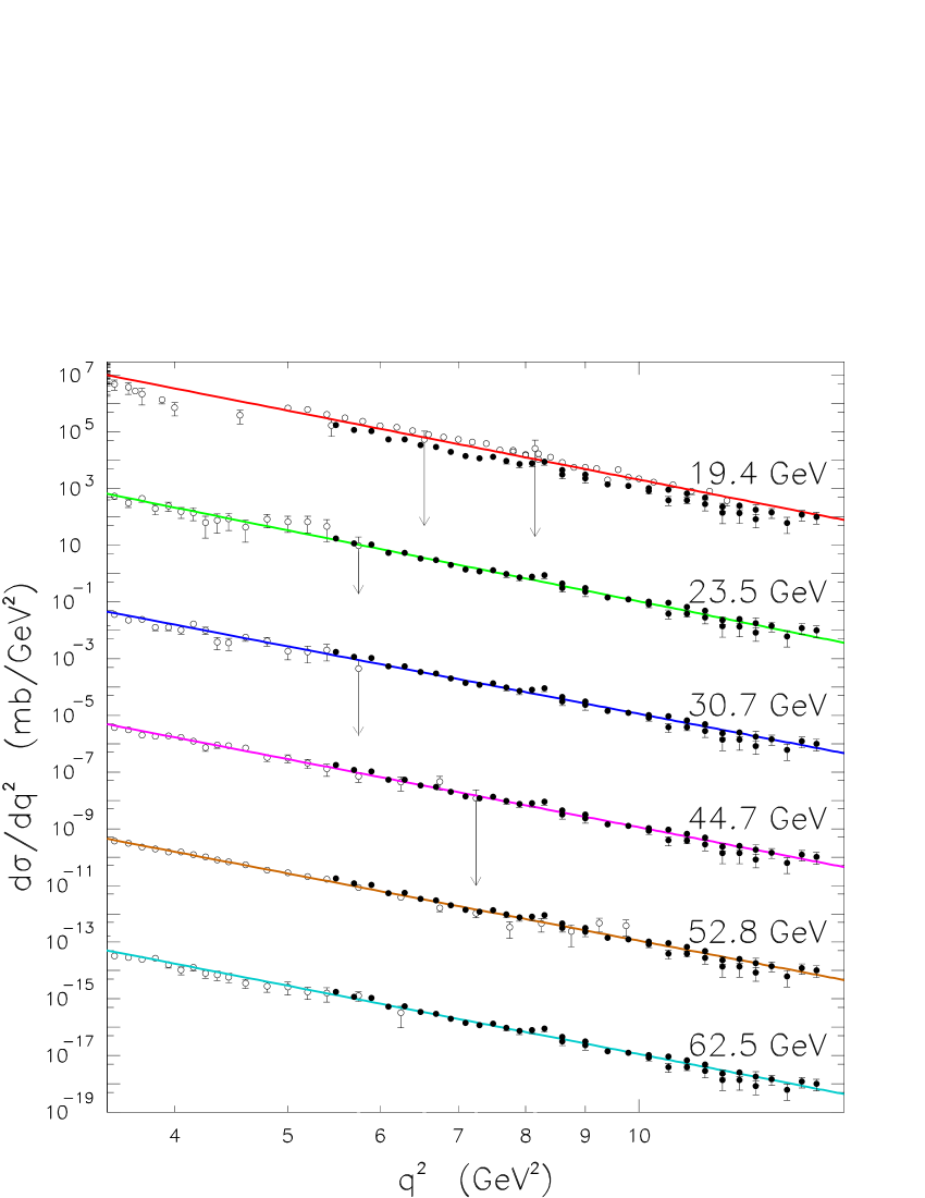
Figure 4: Addition of the data at 27.4 GeV and fit through parametrization (10) in logarithmic scales, with cutoff at $q_{\mathrm{min}}^{2}$ = 3.5 GeV². Curves and data were multiplied by factors of $10^{\pm 4}$.

These tests indicate the following features concerning the energy dependence of each set:

(1) The data at 19.4 GeV are not compatible with the power law and with data at 27.4 GeV since in all the cases (3 cutoffs) $\chi^{2}/DOF\sim$ 20 for $\sim$ 50 $DOF$;

(2) As expected the best statistical results were obtained with $\lambda$ as a free parameter. In this case, their values deviate from 8 as the cutoff increases, reaching $\lambda\sim$ 8.4 for $q_{\mathrm{min}}^{2}$ = 5.5 GeV² (compatible with the numerical value presented by Faissler et al.).

(3) Each set at the ISR energy region is compatible with the power law and with data at 27.4 GeV (the last column shows the average $\chi^{2}/DOF$ at the ISR region). Although the data at 23.5 GeV cover the region up to 5.75 GeV² and those at 27.4 GeV starts at 5.5 GeV² the fits indicate a global compatibility for cutoffs at 3.5 and 4.5 GeV². For that reason we may consider the data at 23.5 GeV as a limit point for the beginning of the energy independence.

These conclusions can be corroborated by performing the same test with all the ISR data together and then by adding to this ensemble the data at 27.4 GeV. For completeness we also consider the fit to data at 19.4 GeV alone. The results with cutoff at 3.5 GeV² are displayed in Table 4, where the above ensembles are denoted by ISR, ISR + 27.4 and 19.4, respectively. Figure 5 shows the fit result in the case of the ensemble ISR + 27.4 and $\lambda$ as a free fit parameter.

Table 4: Fits through parametrization (10) to: (1) all the ISR data (ISR); (2) all the ISR data together with data at 27.4 GeV (ISR + 27.4); (3) data at 19.4 GeV (19.4).

Ensemble	$DOF$	$\chi^{2}/DOF$	$K$ (mbGeV-2)	$\lambda$
ISR	$90$	$0.97$	$0.09635\pm 0.00096$	8
	$89$	$0.87$	$0.085\pm 0.013$	$7.91\pm 0.11$
ISR + 27.4	$129$	$1.46$	$0.1012\pm 0.0014$	8
	$128$	$1.38$	$0.0798\pm 0.0055$	$7.847\pm 0.042$
19.4	$43$	$10.0$	$0.2571\pm 0.0021$	8
	$42$	$11.3$	$0.258\pm 0.017$	$8.003\pm 0.032$

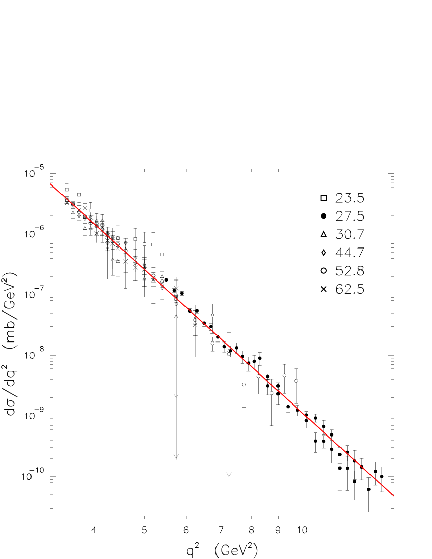
Figure 5: Fit to $pp$ differential cross section data from ISR together with data at 27.4 GeV (ISR + 27.4) and $q^{2}>$ 3.5 GeV².

The main conclusion, for what follows, is that the data at 27.4 GeV can be added to each of the 5 ISR data sets, leading to ensembles with improved experimental information in the region of the large momentum transfers ($q_{\mathrm{max}}^{2}$ = 14.2 GeV² in all the cases), reducing the uncertainties in the extrapolated fits. That, however, is not the case of data at 19.4 GeV, for which $q_{\mathrm{max}}^{2}$ = 11.9 GeV².

4 Improvements in the previous analysis and fit results

Now we first discuss some improvements introduced in the previous analyses cmm ; cm , which are based on three aspects: the data ensemble (selected data) and fit procedure, the structure of the parametrization and the confidence intervals for the uncertainties in the fit parameters. After that we present our new fit results.

4.1 Data ensembles and energy independence

Based on all the information and comments presented in Sect. 3, we call the attention here to two errors appearing in cmm ; cm and discuss the corrections needed. These concern the selected data at 19.4 and 27.4 GeV, as well as the criterion for the energy independence at large momentum transfer.

First, in References cmm and cm the data set at 27.4 GeV was extracted from the LB tables and as we have seen, these 30 data points do not correspond to the final result with 39 points published by Faissler et al. (Sect. 3.3.1). Here we make use of this latter data set.

Secondly, in cmm the data at 19.4 GeV covers only the region up to 8.15 GeV² since the data by Faissler et al. at this energy (up to 11.9 GeV²) were not included in the analysis. Here, as referred to in Sect. 3.2.1 we include all the data available at this energy.

Finally, in the fit procedure developed in cmm the data at 27.4 GeV were added to the data set at 19.4 GeV. However, as we have discussed, there is no statistical justification for this addition due to energy dependence present in this region.

As we shall show in the next sections, these corrections play an important role in the fit results, specially in the statistical evidence for eikonal zeros and the dependence of the position of the zeros on the energy.

4.2 Parametrization

In cmm and cm the parametrization for the real and imaginary parts of the scattering amplitude was expressed in terms of a sum of exponential in $q^{2}$ and the experimental $\rho$ value at each energy as input. Here we use the same basic form but include also the the total cross section as input parameter. Specifically, the scattering amplitude, $F(s,q)=\mathrm{Re\>}F(s,q)+\mathrm{i}\mathrm{Im\>}F(s,q)$, is parametrized by

$$F(s,q)=\mu(s)\sum_{j=1}^{m}\alpha_{j}e^{-\beta_{j}q^{2}}+\mathrm{i}\sum_{j=1}^{n}\alpha_{j}e^{-\beta_{j}q^{2}},$$ (11)

where here,

$$\mu(s)=\frac{\rho(s)\sigma_{\mathrm{tot}}(s)}{4\pi\sum_{j=1}^{m}\alpha_{j}},$$ (12)

and $\rho(s)$ and $\sigma_{\mathrm{tot}}(s)$ are the experimental values at each energy. In this way the parametrization now reproduces both Eqs. (5) and (6).

4.3 Confidence intervals for uncertainties

Another improvement concerns the confidence level for estimating the errors in the fit parameters (variances and covariances). In cmm ; cm the errors correspond to an increase of the $\chi^{2}$ by one unity, which is controlled in the CERN-Minuit code by the up parameter, being set equal to 1. Depending on the number of free parameters, this fixed value implies in different confidence level intervals, which determine the interval of the uncertainty in each free parameter minuit . With this procedure, any error propagation is different for fits with different number of parameters. Here, on the other hand, we fixed the confidence interval using the corresponding up value for each number of parameters. Specifically, the errors in the fit parameters correspond to the projection of the $\chi^{2}$ hypersurface containing 70% of probability in each energy analyzed.

4.4 Fit results

Summarizing, we analyze six ensembles of data on $pp$ differential cross sections: the set at 19.4 GeV and the five sets at the ISR energies with the data at 27.4 GeV added to each set. The data cover the region above the Coulomb-nuclear interference and include the optical points (Table 1). The errors are the statistical only.

Each set was fitted through parametrization (11-12), with the experimental values of $\sigma_{\mathrm{tot}}(s)$ and $\rho(s)$ at each energy (Table 1), by means of the CERN-Minuit code. The best fits were obtained with 2 exponential in the real part and 4, 5 or 6 in the imaginary part depending on the data set analyzed: $m=2$ and $n=4$, $5$ or $6$ in Eq. (11). We note that the exponential terms with $j=1$ and $j=2$ appears in both the real and imaginary parts.

The numerical results of the fits are displayed in Table 5 together with the statistical information, including the value of the $up$ parameter and the values of the $\chi^{2}/DOF$ obtained in the previous analysis cmm . Figures 6 and 7 show the fit results together with the experimental data in the whole $q^{2}$ region and at the diffraction peak, respectively. In Fig. 8 we display the contributions to the differential cross section from the real and imaginary parts of the amplitude.

Table 5: Fit results and statistical information from each data set: values of the free parameters, maximum value of the momentum transfer in GeV² ($q_{\mathrm{max}}^{2}$), values of the $up$ parameter for each fit (see text), number of degrees of freedom ($DOF$) and chi square per degree of freedom ($\chi^{2}/DOF$) obtained in this analysis and that obtained in cmm .

$\sqrt{s}$ (GeV):	19.4	23.5	30.7	44.7	52.8	62.5
$\alpha_{1}$	0.1364	-0.260	$-1.20\times 10^{-3}$	-0.0119	-0.0281	-0.042
	$\pm$ 0.0041	$\pm$ 0.074	$\pm 0.87\times 10^{-3}$	$\pm$ 0.0024	$\pm$ 0.0045	$\pm$ 0.014
$\alpha_{2}$	-1.655	3.4	3.70	0.631	1.26	2.20
	$\pm$ 0.066	$\pm$ 1.3	$\pm$ 0.49	$\pm$ 0.090	$\pm$ 0.13	$\pm$ 0.61
$\alpha_{3}$	3.686	0.25	-0.0441	3.710	3.631	0.20
	$\pm$ 0.069	$\pm$ 0.13	$\pm$ 0.0063	$\pm$ 0.053	$\pm$ 0.060	$\pm$ 0.28
$\alpha_{4}$	-1.495	-	-	-3.096	-3.116	-
	$\pm$ 0.042			$\pm$ 0.050	$\pm$ 0.056
$\alpha_{5}$	7.396	-0.0014	4.51	7.425	6.996	6.46
	$\pm$ 0.086	$\pm$ 0.0017	$\pm$ 0.51	$\pm$ 0.075	$\pm$ 0.012	$\pm$ 0.64
$\alpha_{6}$	-0.1093	4.6	-	$-0.39\times 10^{-3}$	$-1.06\times 10^{-3}$	-0.0013
	$\pm$ 0.0040	$\pm$ 1.3		$\pm 0.38\times 10^{-3}$	$\pm 0.54\times 10^{-3}$	$\pm$ 0.0013
$\beta_{1}$	0.6002	1.19	0.378	0.736	0.926	0.98
	$\pm$ 0.0060	$\pm$ 0.29	$\pm$ 0.067	$\pm$ 0.049	$\pm$ 0.051	$\pm$ 0.14
$\beta_{2}$	2.762	8.4	8.18	31.6	16.5	11.6
	$\pm$ 0.063	$\pm$ 1.7	$\pm$ 0.62	$\pm$ 6.4	$\pm$ 1.6	$\pm$ 1.9
$\beta_{3}$	2.272	1.31	0.984	2.183	2.217	2.89
	$\pm$ 0.017	$\pm$ 0.54	$\pm$ 0.079	$\pm$ 0.014	$\pm$ 0.015	$\pm$ 0.94
$\beta_{4}$	1.770	-	-	2.063	2.126	-
	$\pm$ 0.017			$\pm$ 0.013	$\pm$ 0.014
$\beta_{5}$	5.864	0.39	4.21	6.092	5.646	5.18
	$\pm$ 0.077	$\pm$ 0.11	$\pm$ 0.12	$\pm$ 0.086	$\pm$ 0.086	$\pm$ 0.25
$\beta_{6}$	0.5706	4.24	-	0.292	0.368	0.382
	$\pm$ 0.0046	$\pm$ 0.44		$\pm$ 0.081	$\pm$ 0.048	$\pm$ 0.092
$q_{\mathrm{max}}^{2}$ (GeV2)	11.9	14.2	14.2	14.2	14.2	14.2
$up$	14.02	11.78	9.52	14.02	14.02	11.78
$DOF$	145	163	204	235	233	154
$\chi^{2}/DOF$	2.76	1.20	1.24	2.05	1.71	1.22
$\chi^{2}/DOF$ in cmm	2.80	1.20	1.28	2.13	2.07	1.51

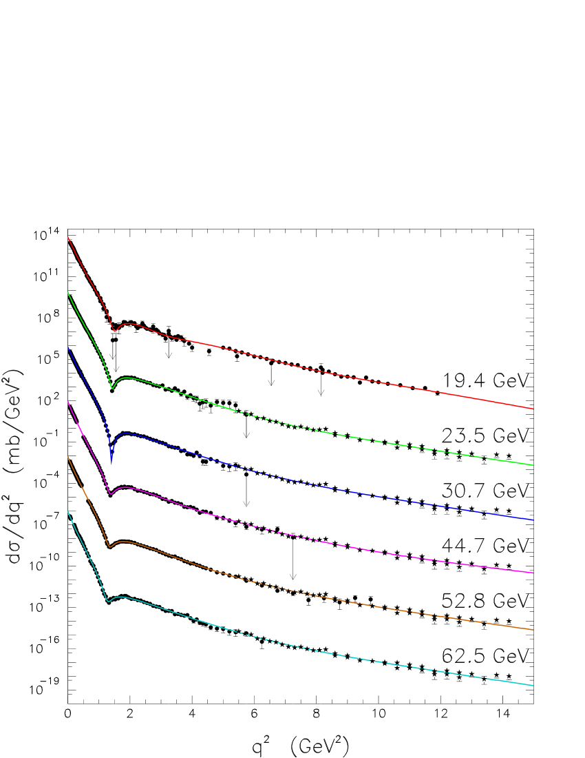
Figure 6: Results of the fits to $pp$ differential cross section data. Curves and data were multiplied by factors of $10^{\pm 4}$.

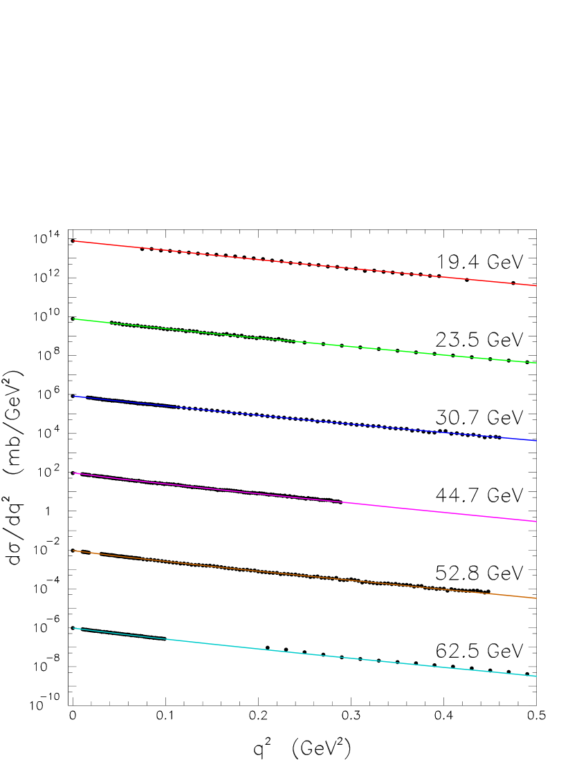
Figure 7: Results of the fit at the diffraction peak. Curves and data were multiplied by factors of $10^{\pm 4}$.

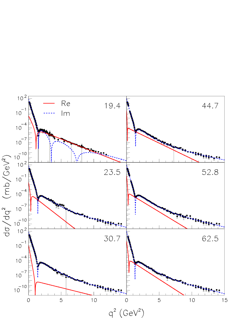
Figure 8: Contributions to the differential cross sections from the real (dotted) and imaginary (dashed) parts of the amplitude.

From Table 5 we see that the values of the $\chi^{2}/DOF$ here obtained are slightly small than those presented in cmm , except at 23.5 GeV for which the value is the same. This slight improvement in the statistical result may be due to the inclusion of the $\sigma_{\mathrm{tot}}$ experimental data in the parametrization at each energy. From Fig. 8 we see that in all the cases the real part of the amplitude presents one zero at small values of the momentum transfers, a result in agreement with the theorem by Martin for the real amplitude martin . The imaginary part develops one zero at the ISR energies and multiple zeros at 19.4 GeV and that may be due to the fact that these data are not normalized as in the analysis by Amaldi and Schubert. This effect at 19.4 did not appear in the previous analysis cmm due to the unjustified addition of data at 27.4 GeV.

5 Eikonal in the momentum transfer space

The point in the extraction of the eikonal is not only its determination in the $q$ space, through the steps described in Sect. 2, but mainly the estimation of the uncertainty regions by means of propagation of the errors in the fit parameters (variances and covariances) and also the errors from $\sigma_{\mathrm{tot}}(s)$ and $\rho(s)$. The problem here is that, with parametrizations like (11 - 12) for the scattering amplitude (sum of exponential in $q^{2}$), the translation of the eikonal from $b$-space to $q$-space, Eq. (3), can not be analytically performed and therefore, the standard error propagation neither. To solve this problem a semi-analytical method was developed, which is explained in detail in cmm ; cm and will also be applied in this analysis.

In what follows we shall treat only the imaginary part of the eikonal since, according to our definition, Eqs. (1) and (2), it corresponds to a real opacity function in the optical analogy. With the usual notation we represent

$$\mathrm{Im\>}\chi(s,b)\equiv\Omega(s,b).$$ (13)

We shall also use the bracket $<\ >$ to denote two dimensional Fourier transform with azimuthal symmetry, so that the translations between $q$ and $b$ spaces will be expressed by

$$\Omega(s,b)=<\tilde{\Omega}(s,q)>=\int_{0}^{\infty}q\mathrm{d}qJ_{0}(qb)\tilde{\Omega}(s,q),$$ (14)

$$\tilde{\Omega}(s,q)=<\Omega(s,b)>=\int_{0}^{\infty}b\mathrm{d}bJ_{0}(qb)\Omega(s,b).$$ (15)

5.1 Semi-analytical method

As shown in cmm , taking into account the error propagation from the fit parameters it is possible to approximate the imaginary part of the eikonal in Eq. (8) by

$$\Omega(s,b)\approx\ln\left[\frac{1}{1-\mathrm{Re}\ \Gamma(s,b)}\right]$$ (16)

and the same is valid in the present analysis. Expanding this equation we obtain

$$\Omega(s,b)=\mathrm{Re}\ \Gamma(s,b)+R(s,b),$$ (17)

where $R(s,b)$ represents the remainder of the series:

$$R(s,b)=\ln\left[\frac{1}{1-\mathrm{Re}\ \Gamma(s,b)}\right]-\mathrm{Re}\ \Gamma(s,b).$$ (18)

Up to this point the errors of fit parameters from $\mathrm{Im}\ F$ can be propagated to $\mathrm{Re}\ \Gamma$ by Eq. (7) and to $R(s,b)$, Eq. (18). The next step concerns the translation of Eq. (17) from $b$-space to $q$-space, Eq. (15). Applying the Fourier transform in (17) we obtain

$$\tilde{\Omega}(s,q)=\mathrm{Im}\ F(s,q)+\tilde{R}(s,q).$$ (19)

As commented on before, the point here is that due to the structure of the parametrization, the translation from $R(s,b)$ to $\tilde{R}(s,q)$ can not be performed in an analytical way and as consequence nor can the error propagation. The semi-analytical method introduced in cm address this question through the following procedure. We first generate an ensemble of numerical points $R(s,b)$ through Eq. (18), with propagated errors $\pm\Delta R(s,b)$ and then fit this ensemble by a sum of gaussians in $b$, in practice with six terms:

$$R_{\textrm{fit}}\>(s,b)=\sum_{j=1}^{6}A_{j}\mathrm{e}^{-B_{j}b^{2}}.$$ (20)

In this way, not only $\tilde{R}(s,q)$ can be evaluated through the Fourier transform of the above formula, but also the errors from the fit parameters $A_{j}$, $B_{j}$, can be analytically propagated providing $\Delta\tilde{R}$ and, through Eq. (19), $\Delta\tilde{\Omega}(s,q)$. As discussed in cmm , this method allows the study of several aspects of the eikonal in the momentum transfer space. In this work we shall focus only on the investigation of eikonal zeros (change of sign).

5.2 Eikonal zeros

A review on previous indication of eikonal zeros, with complete references to outstanding results can be found in cmm . Here we use the semi-analytical method in order to investigate the eikonal zeros and the associated uncertainties. As in cmm ; cm that can be done through plots of $q^{8}$ times $\tilde{\Omega}(s,q)\pm\Delta\tilde{\Omega}(s,q)$ as function of the momentum transfer as shown in Fig. 9. We consider as statistical evidence of a change of signal only the cases in which the uncertainty region above the central value is below the zero. With this criterion, from Fig. 9, we have evidence for the change of sign at all the ISR energies, but, different from the result obtained in cmm , not at $\sqrt{s}$ = 19.4 GeV.

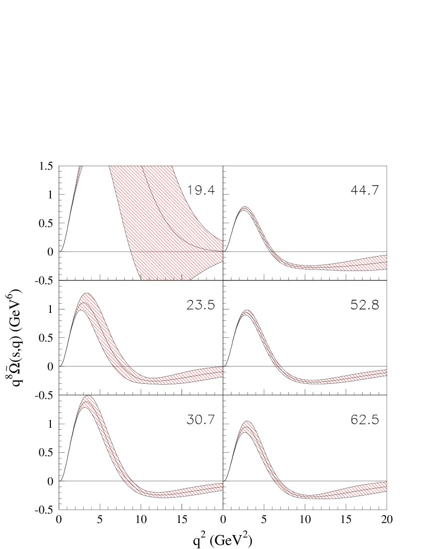
Figure 9: Imaginary part of the Eikonal in the momentum transfer space multiplied by $q^{8}$ and uncertainty regions from error propagation.

We recall that in cmm the data at 27.4 GeV was added to those at 19.4 GeV and that is not the case here. This suggest the importance of data at large momentum transfer in statistical identification of a zero in the eikonal. This aspect can also be corroborated if we consider fits only to the original ISR data sets, that is, without adding the data at 27.4 GeV. The results with parametrization (11-12) are displayed in Fig. 10, from which we see that except for the data at 44.7 and 52.8 GeV no evidence of zeros can be inferred and these two sets just correspond to those with the largest interval in the momentum transfer with available data (Fig. 1).

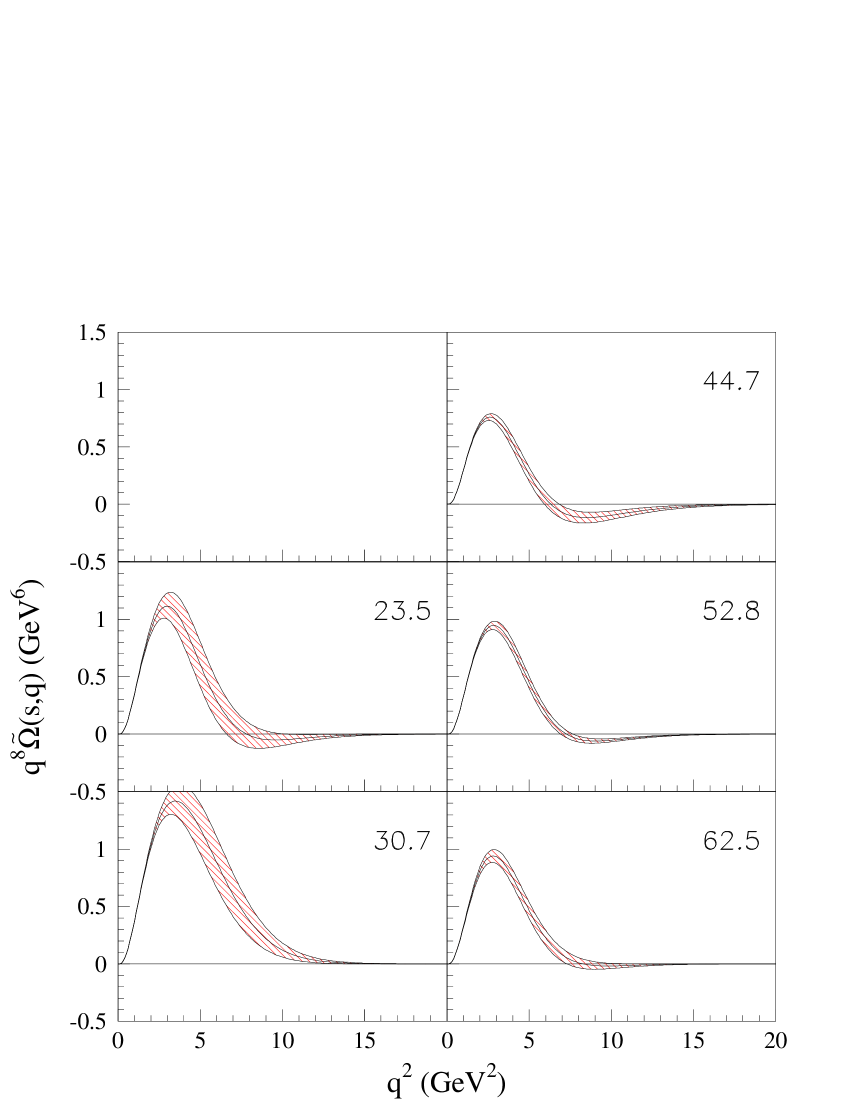
Figure 10: Same as Fig. 9 from fits to the ISR data sets without adding the data at 27.4 GeV.

From the plots in Fig. 9 and the NAG routine (C05ADF), we can determine the position of the zeros and the uncertainties associated with each central value by means of the extrema intervals of the propagated errors (asymmetrical). The numerical results extracted in this way are shown in Table 6, where $q_{0}^{2}$ indicates the central value of the zero and $+\Delta q_{0}^{2}$ and $-\Delta q_{0}^{2}$ the asymmetrical uncertainties at the right and the left of the central value, respectively. These numerical values are plotted in Fig. 11, where the lines connecting the central values were drawn only to guide the eye.

Table 6: Position of the eikonal zero ($q_{0}^{2}$) and the asymmetrical uncertainties ($+\Delta q_{0}^{2}$ and $-\Delta q_{0}^{2}$) in terms of the energy.

$\sqrt{s}$ (GeV)	$q_{0}^{2}$	$-\Delta q_{0}^{2}$	$+\Delta q_{0}^{2}$ (GeV2)
23.5	7.72	1.07	0.88
30.7	8.54	0.99	0.80
44.7	5.83	0.15	0.16
52.8	6.74	0.64	0.60
62.5	6.63	0.37	0.35

Figure 11: Position of the eikonal zero and uncertainties in terms of the energy (Table 6).

Despite the statistical evidence for the change of sign of the eikonal at the ISR energy region, these results do not allow one to extract a quantitative correlation between the position of the zero, $q_{0}^{2}$, and the energy. However, we can outline the following quantitative features:

(1) For the lower energies ($\sqrt{s}$ = 23.5 and 30.7 GeV²) $q_{0}^{2}\sim$ 8 GeV² and for the higher energies (44.7, 52.8 and 62.5 GeV) $q_{0}^{2}\sim$ 6 GeV², suggesting a decreasing in the position of the zero as the energy increases.

(2) Fits to the data on the zero position, Table 6, with a linear function, $q_{0}^{2}=a+b\ln s$ gives $q_{0}^{2}=(12.3\pm 2.9)-(0.74\pm 0.37)\ln s$, with $\quad\chi^{2}/DOF=$ 5.3, if the largest errors are used and $q_{0}^{2}=(12.8\pm 2.6)-(0.81\pm 0.3)\ln s$, with $\quad\chi^{2}/DOF=$ 6.0, in the case of the smallest errors. Since the errors in the slopes are about 50 % of the central value, these results also suggest a decreasing in $q_{0}^{2}$ as the energy increases.

(3) If we assume $b=0$ in the above parametrizations (null slope) we obtain, respectively, $q_{0}^{2}=6.60\pm 0.16$ GeV², $\chi^{2}/DOF=$ 5.0 and $q_{0}^{2}=6.61\pm 0.15$ GeV², $\chi^{2}/DOF$= 6.0.

(4) The average of only the central values gives $\bar{q_{0}^{2}}=7.04\pm 1.08$ GeV².

From these numerical results we can only infer the evidence of the change of sign in the eikonal in the region 6 - 8 GeV², what can roughly be represented by the value:

$$\bar{q_{0}^{2}}=7.0\pm 1.0\ \mathrm{GeV}^{2}.$$ (21)

We note that the conclusion that the position of the zero decreases with the increasing of the energy, inferred in cmm , was based on the position of the zero at $\sqrt{s}$ = 19.4 GeV, namely $q_{0}^{2}\approx$ 9 GeV² (see Fig. 15 in that reference). However, without adding the data at 27.4 GeV, as we did here, we can not infer this result. In what follows we discuss the implication of this zero in the phenomenological context.

6 Phenomenological implication of the eikonal zeros

First, an important observation. Despite the detailed model independent analysis here developed, it should be stressed that we do not present $the$ empirical result, but $an$ empirical result. In fact, even with the justified strategy of adding data at large momentum transfer, the fit procedure has, in principle, an infinity number of solutions. In our case, this drawback is mainly associated with the lack of knowledge of the contributions from real and imaginary parts of the amplitude beyond the forward direction, which represents a serious challenge in any inverse scattering problem. For that reason, in what follows, we shall base our general discussion in qualitative aspects, treating also some quantitative features but without going into details.

Summarizing, our model independent result for the imaginary part of the eikonal in the $q$ space indicates that, at the ISR region, the eikonal is positive up to $q_{0}^{2}\sim$ 7 GeV², changes sign at this point, has a negative minimum above the zero position and then goes to zero through negative values (Fig. 9). As already discussed by Kawasaki, Maheara and Yonegawa kmy this behavior suggests two distinct dynamical contributions in the diffractive regime: an interaction with long range (positive eikonal below the zero) and another with short range (negative eikonal above the zero). In this Section we discuss some implication of this behavior. We first treat empirical results related with the eikonal and the scattering amplitude (Sect. 6.1) and then the implication on the zero in terms of eikonal models (Sect. 6.2) and form factors (Sect. 6.3).

6.1 Eikonal and scattering amplitude

One of the most important label of elastic hadron scattering as a diffractive process is the diffraction pattern in the differential cross section: the peak, the dip and the smooth decrease at large momentum transfer. It is generally accepted that the dip at $q^{2}\sim$ 1.5 GeV² (Figures 1 and 2) is due to a change of sign (zero) in the imaginary part of the amplitude and that the dip is filled up by the real part of the amplitude. That is, at least, what our fit results indicate (Fig. 8). Therefore it may be worthwhile to examine possible connections between the zeros in the amplitudes and in the eikonal (imaginary parts). Several interesting aspects of this subject have already been discussed by Kawasaki, Maehara and Yonezawa kmy ; here we focus only on our empirical results.

By expanding the exponential term in Eq. (1) we obtain for the imaginary part of the amplitude

$$\mathrm{Im\>}F(s,q)=\mathrm{Im}<\chi(s,b)>+\frac{1}{2!}\mathrm{Re}<\chi^{2}(s,b)>$$ (22)

$$- \frac{1}{3!}\mathrm{Im}<\chi^{3}(s,b)>-\frac{1}{4!}\mathrm{Re}<\chi^{4}(s,b)>+....$$

Therefore, in principle, the zero in $\mathrm{Im\>}F(s,q)$ can be generated either by a zero in $\tilde{\Omega}(s,q)=\mathrm{Im}<\chi(s,b)>$ or by the terms with alternating signs in the series kmy . Obviously the difference between $\mathrm{Im\>}F$ and $\tilde{\Omega}$ (the leading term) comes from the contribution of the reminder of the series.

Quantitative information on this respect can be obtained directly from our fit results and by comparing both quantities (amplitude and eikonal). To this end we consider, as in the case of the eikonal in the $q$-space, the product of $q^{8}$ by $\mathrm{Im\>}F(s,q)$ for all the energies analyzed as shown in Fig. 12. With this we can determine the position of the zero in the amplitude together with the propagated uncertainties. The results are displayed in Fig. 13 and Table 7 (where the value at 19.4 GeV corresponds to the first zero only).

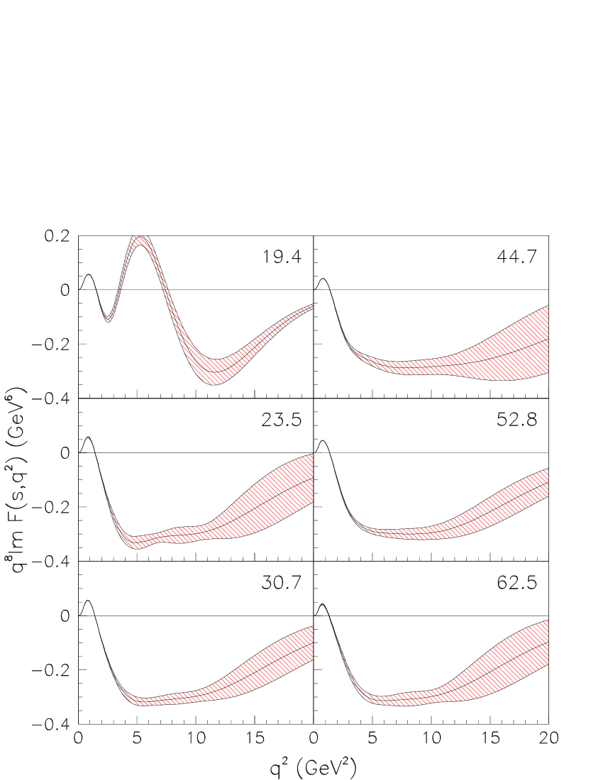
Figure 12: Fit results for the imaginary part of the amplitude, multiplied by $q^{8}$ and uncertainty regions from error propagation (analogous to Fig. 9 for the imaginary part of the eikonal).

Table 7: Position of the zero in the imaginary part of the amplitude (first zero in the case of 19.4 GeV).

$\sqrt{s}$ (GeV)	$q_{0}^{2}$	$-\Delta q_{0}^{2}$	$+\Delta q_{0}^{2}$ (GeV2)
19.4	1.528	0.014	0.015
23.5	1.4325	0.0095	0.0097
30.7	1.4147	0.0071	0.0071
44.7	1.377	0.010	0.010
52.8	1.3520	0.0094	0.0097
62.5	1.297	0.021	0.019

Figure 13: Position of the zero in the imaginary part of the amplitude. At 19.4 GeV the value corresponds to the first zero (Table 7).

These results allow to extract the following empirical features:

(1) Concerning the position of the zero in the amplitude and in the eikonal, Tables 6 and 7 and Figs. 11 and 13 show that there is no correlation at all between them: in contrast with the position of the zero in the amplitude, which systematically decreases as the energy increases (an effect related to the well known shrinkage of the diffraction peak), the eikonal zero has an approximately constant position in the energy region investigated.

(2) At 19.4 GeV, from Fig. 9 for the eikonal, we see that it is not possible to identify a change of sign on statistical grounds (uncertainties below the zero), nor in terms of the central value neither since it goes asymptotically to zero through positive values. From Fig. 12, the corresponding imaginary part of the amplitude presents multiple zeros (three at finite $q^{2}$-values and one asymptotically, through negative values).

(3) At the ISR energy region, from Fig. 9, we have evidence for the change of signal (one zero) and the corresponding imaginary part of the amplitudes, Fig. 12, also present only one change of signal at fixed $q^{2}$, going to zero through negative values.

The last two features suggest that a positive-definite eikonal in the $q$ space originates in multiple dips in the corresponding differential cross section (zeros in the imaginary part of the amplitude); on the other hand, an eikonal with one change of signal, gives rise to only one dip and a smooth decrease at large momentum transfers. In what follows we discuss these effects in the context of some eikonal models.

6.2 Some representative eikonal models

In order to illustrate the empirical features described above, we have chosen some representative and popular eikonal models, characterized by parametrizations with and without zero in the imaginary part of the eikonal in the $q$ space. We first review some aspects of each model we are interested in (Sects. 6.2.1 - 6.2.3) and then discuss the connections with the empirical results (Sect. 6.2.4).

6.2.1 Models without eikonal zero

Representatives of this class are the historical Chou-Yang model wy ; by ; dl ; cy ; cy90 and some recent QCD-inspired models bghp ; lmmmn . Due to the importance of the connections between eikonal and form factors and for further discussion (Sect. 6.3), we recall some details of the droplet model by Yang and collaborators and only briefly quote some inputs of interest in QCD models.

$\bullet$ Chou-Yang model

Basic concepts. In this model, the internal structure of a hadron is assumed to be described by a density of opaqueness $\rho(x,y,z)$ and in a collision, relativistic effects imply in a contraction of the extended object, so that, in the center-of-mass frame each hadron “sees” the other as a two-dimensional matter distribution,

$$D(x,y)=\int_{-\infty}^{+\infty}\rho(x,y,z)\mathrm{d}z,$$

where $x$ and $y$ lie on the impact parameter plane and $z$ is the coordinate perpendicular to it. According to the optical analogy, the resultant opaqueness (the imaginary part of the eikonal) in the collision of hadrons $A$ and $B$ is assumed to be the overlapping (convolution) of the matter distributions,

$$\Omega_{AB}(s,b) = C_{AB}\int\mathrm{d}^{2}\vec{b^{\prime}}D_{A}(|\vec{b^{\prime}}|)D_{B}(|\vec{b^{\prime}}-\vec{b}|)$$ (23)

$$\equiv C_{AB}\ D_{A}\otimes D_{B},$$

where $C_{AB}$ is impact parameter independent (it depends on the energy), and $D_{A,B}$ are connected to the hadronic matter form factors,

$$G_{A,B}(\vec{q})=\int\mathrm{e}^{\mathrm{i}\vec{q}\cdot\vec{r}}\rho_{A,B}(\vec{r})\mathrm{d}\vec{r},$$ (24)

through the Fourier transform,

$$D_{A,B}(b)=<G_{A,B}(q)>.$$ (25)

From the convolution theorem, we obtain the formal expression of the eikonal in the impact parameter space:

$$\Omega_{AB}(s,b)=C_{AB}(s)<G_{A}(q)G_{B}(q)>.$$ (26)

The Wu-Yang conjecture. In 1965, based on heuristic arguments, Wu and Yang speculated that the elastic $pp$ differential cross sections might be proportional to the fourth power of the proton charge form factor wy , that is the form factor measured in electron-proton scattering. The connection with this power of the form factor is obtained, in the above model, by considering the first order expansion of the eikonal, Eqs. (22) and (26), since for the proton case:

$$\mathrm{Im\>}F(s,q)\propto G_{p}^{2}.$$ (27)

Several electromagnetic form factors and inverse scattering problems were discussed in the subsequent years by ; dl ; cy , including the traditional dipole parametrization for the Sachas electric form factor dl

$$G_{D}(q)=\frac{1}{[1+q^{2}/\mu^{2}]^{2}},\qquad\mu^{2}=0.71\ {\rm GeV}^{2}.$$ (28)

In this case, from Eq. (26), the opacity in the impact parameter space for $pp$ scattering reads

$$\Omega(s,b)=C(s)\frac{(\mu b)^{3}}{8}K_{3}(\mu b),$$ (29)

where $K_{3}$ is a modified Bessel function. With inputs like that, the absorption factor $C_{AB}(s)$ is the only free parameter, determined from the experimental value of the total cross section at each energy. The main realization of this model was the prediction of the diffraction pattern in $pp$ differential cross section and the correct position of the dip, as experimentally observed later.

However, although efficient in the description of the experimental data, the strong conjecture by Wu and Yang, correlating the hadronic matter form factor with the electric form factor, can not be proved or disproved in the phenomenological context. We shall return to this fundamental point in Sect. 6.3, when discussing recent results on the proton electric form factor.

$\bullet$ QCD-Inspired models

In this class of model bghp ; lmmmn the even eikonal is expressed as a sum of three contributions, from gluon-gluon ($gg$), quark-gluon ($qg$) and quark-quark ($qq$) interactions,

$$\chi^{+}(s,b)=\chi_{gg}(s,b)+\chi_{qg}(s,b)+\chi_{qq}(s,b),$$

which individually factorize in $s$ and $b$,

$$\chi_{ij}(s,b)=\mathrm{i}\sigma_{ij}(s)w(b,\mu_{ij}),$$

where $ij$ stands for $gg$, $qg$ and $qq$. The impact parameter distribution function for each process comes from convolution involving dipole form factors, in the same way as in the Chou-Yang model, Eqs. (23) and (28), but at the elementary level:

$$w_{ii}(b,\mu_{ii})=\int\mathrm{d}^{2}\vec{b^{\prime}}D_{i}(|\vec{b^{\prime}}|)\ D_{i}(|\vec{b^{\prime}}-\vec{b}|),$$

$$G_{ii}(b,\mu_{ii})=\left<\frac{1}{[1+q^{2}/\mu_{ii}^{2}]^{2}}\right>,$$

so that

$$w_{ii}(b,\mu_{ii})=\frac{[\mu_{ii}b]^{3}}{8}K_{3}(\mu_{ii}b),$$

where, for $i\not=j$:

$$\mu_{ij}\equiv\sqrt{\mu_{ii}\mu_{jj}}.$$

Therefore, in the momentum transfer space, the imaginary part of the eikonal has the same structure of the Chou-Yang model, with the dipole parametrization and the scale factors $\mu_{ii}$, $i=g,q$ as free fit parameters, depending also on the elementary process ($qq$ or $gg$). With several other ingredients this class of model allows for good descriptions of the forward data and differential cross section data at small momentum transfers bghp ; lmmmn .

6.2.2 Hybrid model

For further discussion we also recall a particular model with different parametrizations for $pp$ scattering at the ISR region and $\bar{p}p$ scattering at the Collider energies, the former using an eikonal with multiple zeros and the later without zero. The model, developed by Glauber and Velasco gv1 ; gv2 , is based on Glauber’s multiple diffraction formalism which, in leading order, introduces the following expression for the eikonal glauber

$$\tilde{\chi}(s,q)=\sum_{i=1}^{N_{A}}\sum_{j=1}^{N_{B}}G_{A}G_{B}f_{ij},$$

where $G_{A}$ and $G_{B}$ are the hadronic form factors, $N_{A}$ and $N_{B}$ the number of constituents in each hadron and $f_{ij}$ the individual elementary scattering amplitudes between the constituents (parton-parton scattering amplitudes). In the case that the elementary amplitudes can be considered to be the same, denoted by $f$, and that $N_{A}N_{B}\equiv N$, we have for the imaginary part

$$\tilde{\Omega}(s,q)=NG_{A}G_{B}\mathrm{Im}f.$$ (30)

In the Glauber-Velasco version gv1 ; gv2 use is made of the Felst as well as the Borkowski-Simon-Walther-Wendling (BSWW) form factors (no zeros), together with the following parametrization for the imaginary part of the elementary amplitude in the case of $\bar{p}p$ scattering at 546 GeV gv1 :

$$f(q)=\frac{1}{[1+q^{2}/a^{2}]^{1/2}}.$$

Therefore, the eikonal presents no zero. For $pp$ scattering at 23.5 a phase factor was introduced,

$$f(q)=\frac{\exp{\{\mathrm{i}[b_{1}q^{2}+b_{2}q^{4}]\}}}{[1+q^{2}/a^{2}]^{1/2}}$$

and in this case both the real an imaginary parts of the eikonal present multiple zeros. For further reference we recall that the data cover the region up to 5.5 GeV² ($pp$, 23.5 GeV) and 1.6 GeV² ($\bar{p}p$, 546 GeV), that is, not large values of the momentum transfer.

6.2.3 Models with eikonal zero

This is a restrict class of eikonal models. We shall consider here the impact parameter picture by Bourrely, Soffer and Wu and a geometrical or multiple diffraction approach.

$\bullet$ Bourrely-Soffer-Wu model

The impact parameter picture by Bourrely-Soffer-Wu (BSW) bsw ; bsw03 is the most popular and, to our knowledge, the first model to consider an eikonal zero in the momentum transfer space. In this model the eikonal in the impact parameter space is expressed as a sum of two terms

$$\chi(s,b)=R(s,b)+H(s,b),$$

where the first term is a Regge background, which takes into account the differences between $pp$ and $\bar{p}p$ scattering and is parametrized as

$$<R(s,b)>=[c_{+}+c_{-}\mathrm{e}^{-\mathrm{i}\pi\alpha(q^{2})}]s^{\alpha(q^{2})},$$

$$\alpha(q^{2})=\alpha_{0}-\alpha^{\prime}q^{2},\qquad q^{2}=-t.$$

The second term, responsible for the diffractive component (pomeron exchange), is the same for $pp$ and $\bar{p}p$ and factorizes in $s$ and $b$:

$$H(s,b)=S(s)T(b).$$

The energy-dependent term comes from the massive QED and is parametrized in a crossing symmetric form

$$S(s)=\frac{s^{c}}{\ln^{c^{\prime}}s}+\frac{u^{c}}{\ln^{c^{\prime}}u},$$

where $u$ is the third Mandelstam variable. Finally, the impact parameter dependence, which is our interest, is also inspired in the geometrical picture through the convolution

$$T(b)=kD_{A}\otimes D_{B}=k<G^{2}(q^{2})>.$$ (31)

Here, however, the form factor is parametrized as a product of two simple poles multiplied by a function with a zero in the momentum transfer space,

$$G(q^{2})=\frac{1}{[1+q^{2}/\alpha^{2}]}\frac{1}{[1+q^{2}/\beta^{2}]}\sqrt{\frac{1-q^{2}/q_{0}^{2}}{1+q^{2}/q_{0}^{2}}},$$ (32)

where $k$, $\alpha^{2}$, $\beta^{2}$ and $q_{0}^{2}$ are free fit parameters. The function on the right, with a zero at $q^{2}=q_{0}^{2}$, was introduced to account for possible differences between the electromagnetic and hadronic form factors, as well as to correct the dip position bsw . In the last analysis by Bourrely, Soffer and Wu the position of the zero was inferred to be at bsw03

$$q_{0}^{2}\sim 3.45\ \mathrm{GeV}^{2}.$$ (33)

$\bullet$ A multiple diffraction model

Without a theoretical basis as in the case of the BSW model, a multiple diffraction model (Glauber context), introduced in 1988 md ; bcmp , makes use of the following parametrizations for the eikonal in Eq. (30)

$$\tilde{\Omega}(s,q)=C(s)G^{2}(s,q)\mathrm{Im}\ f(q),$$ (34)

with

$$G(s,q) = \frac{1}{[1+q^{2}/\alpha^{2}(s)]}\frac{1}{[1+q^{2}/\beta^{2}]},$$ (35)

$$\mathrm{Im}f(s,q) = \frac{1-q^{2}/q_{0}^{2}}{1+[q^{2}/q_{0}^{2}]^{2}},$$ (36)

where the $N$ factor has been included in $C(s)$. The mathematical structure is very similar to the geometrical ansatz introduced by BSW, except for the dependence of $\alpha^{2}$ on the energy and the square in the $q^{2}/q_{0}^{2}$ term in the denominator. The reason for this square is explained and discussed in mprd . By means of suitable phenomenological parametrizations for $C(s)$ and $\alpha^{2}(s)$ and for

$$q_{0}^{2}=8.20\ \mathrm{GeV}^{2},$$ (37)

good descriptions of the experimental data on elastic $pp$ and $\bar{p}p$ scattering, above 10 GeV, have been obtained ($\beta_{pp}^{2}=1.80$ GeV² and $\beta_{\bar{p}p}^{2}=1.55$ GeV²); the real part of the amplitude can be evaluated either through the Martin formula md ; mblois ; mcjp or by means of derivative dispersion relations applied at the elementary level mm .

In the geometrical context the $\alpha^{2}$ dependence means hadronic form factors depending on the energy, a hypothesis or procedure that was also used in 1990 by Chou and Yang cy90 . A theoretically improved version of this multiple diffraction model, including dual and pomeron aspects, is presented in covoetal .

6.2.4 Discussion

$\bullet$ General aspects

As is known from the original papers, all the above models without zero in the eikonal can only describe the differential cross section data at small values of the momentum transfer, typically below $q^{2}\sim$ 2 GeV² (for example, QCD inspired models bghp ; lmmmn ). Above this region, theoretical curves present multiple dips which are not present in the experimental data (for example, Chou-Yang model cy ; cy90 and Glauber-Velasco model at Collider energies gv1 ).

On the other hand, models with one zero in the eikonal are able to describe quite well the differential cross section data even at large values of the momentum transfer. Examples are the BSW model bsw ; bsw03 and the variants of the multiple diffraction model mblois ; mcjp ; mm ; covoetal .

Therefore, these phenomenological results are in agreement with the conclusions of our empirical analysis, presented in Sect. 6.1: eikonal with zero gives rise to only one dip in the corresponding differential cross section and a smooth decrease at large values of the momentum transfers. In this sense, the model-independent features extracted from our analysis corroborate the ingredients present in the BSW model and the variants of the multiple diffraction model.

$\bullet$ Quantitative aspects

At this point it seems worthwhile to attempt to go further in the investigation on more quantitative connections among model parametrizations with zero and our empirical results for the imaginary part of the eikonal. We stress, however, the critical comment at the beginning of Sect. 6 on the limitation of our model independent results.

The idea is to generate a discrete set of points for the extracted $\tilde{\Omega}(q)$, with the associated uncertainties from error propagation, and compare with model parametrizations presenting one zero. As we shall see, suitable quantities for this comparison are, as before, $q^{8}\tilde{\Omega}(q)$ and also $|\tilde{\Omega}(q)|$.

In what follows we shall consider only the fit results obtained at 52.8 GeV, since the original data set covers the largest region in momentum transfer (up to 9.75 GeV²), has one of the largest number of points (adding data at 27.4 GeV) and the data reduction presented a reasonable $\chi^{2}/DOF$ (Table 5). The empirical results for $pp$ scattering at 52.8 GeV are displayed in Fig. 14 in the form of points with the propagated errors.

As regards models with eikonal zero, we consider the inputs of the BSW model for the impact parameter dependence, Eqs. (31-32) and the original version of the multiple diffraction model, Eqs. (34-36). For further discussion of these two models, we introduce the following notation for the imaginary part of the eikonal at fixed energy:

$$\tilde{\Omega}(q)=\frac{C}{[1+q^{2}/\alpha^{2}]^{2}[1+q^{2}/\beta^{2}]^{2}}f(q),$$ (38)

with either

$$f(q)\rightarrow f_{\mathrm{BSW}}\equiv\frac{1-q^{2}/q_{0}^{2}}{1+q^{2}/q_{0}^{2}},$$ (39)

or

$$f(q)\rightarrow f_{\mathrm{mBSW}}\equiv\frac{1-q^{2}/q_{0}^{2}}{1+[q^{2}/q_{0}^{2}]^{2}},$$ (40)

where the subscript mBSW stands for modified BSW (referring to the square in the denominator). This notation, introduced in mprd , is useful, since it allows for two distinct physical interpretations for the above eikonal, either in the Chou-Yang or Glauber contexts:

1) a product of two form factors each one in the form introduced by BSW (Chou-Yang context)

$$G_{1}(q)=\frac{1}{[1+q^{2}/\alpha^{2}]}\frac{1}{[1+q^{2}/\beta^{2}]}\sqrt{f(q)},$$ (41)

2) a product of two form factors each one parametrized as two simple poles

$$G_{2}(q)=\frac{1}{[1+q^{2}/\alpha^{2}]}\frac{1}{[1+q^{2}/\beta^{2}]},$$ (42)

by an elementary scattering amplitude (Glauber context)

$$f_{\mathrm{BSW}}(q)\quad\mathrm{or}\quad f_{\mathrm{mBSW}}(q).$$ (43)

The point is that, since $q_{0}^{2}$ represents the eikonal zero, in the former case it is associated with the hadronic form factor and in the latter case with the elementary amplitude.

For comparison with our empirical results at 52.8 GeV, we fix $q_{0}^{2}$ in the above formulas to the extracted position of the zero at this energy, namely $6.74$ GeV² (this is also the median of the values displayed in Table 6) and fit the eikonals (38-40) to the generated points by means of the CERN-Minuit code. The free parameters in both cases are $C$, $\alpha^{2}$ and $\beta^{2}$. The results are displayed in Table 8 (2nd and 3rd columns) and Fig. 14, with the following notation:

$$\tilde{\Omega}_{\mathrm{BSW}}(q)\quad\rightarrow\quad\mathrm{Eqs.\ (\ref{eq:38})\ and\ (\ref{eq:39})}$$

$$\tilde{\Omega}_{\mathrm{mBSW}}(q)\quad\rightarrow\quad\mathrm{Eqs.\ (\ref{eq:38})\ and\ (\ref{eq:40})}$$

Table 8: Results of the data reductions to the generated points in Fig. 14 ($pp$ scattering at 52.8 GeV) through different parametrizations for the imaginary part of the eikonal (see text).

	$\tilde{\Omega}_{\mathrm{BSW}}$	$\tilde{\Omega}_{\mathrm{mBSW}}$	$\tilde{\Omega}_{\mathrm{empir}}$
	Eqs. (38) and (39)	Eqs. (38) and (40)	Eq. (44)
$C$ (GeV-2)	11.351 $\pm$ 0.023	11.220 $\pm$ 0.039	11.155 $\pm$ 0.039
$\alpha^{2}$ (GeV2)	0.704 $\pm$ 0.014	0.746 $\pm$ 0.023	0.4534 $\pm$ 0.0093
$\beta^{2}$ (GeV2)	0.704 $\pm$ 0.015	0.746 $\pm$ 0.023	1.497 $\pm$ 0.047
$\chi^{2}/DOF$	207	42	0.50

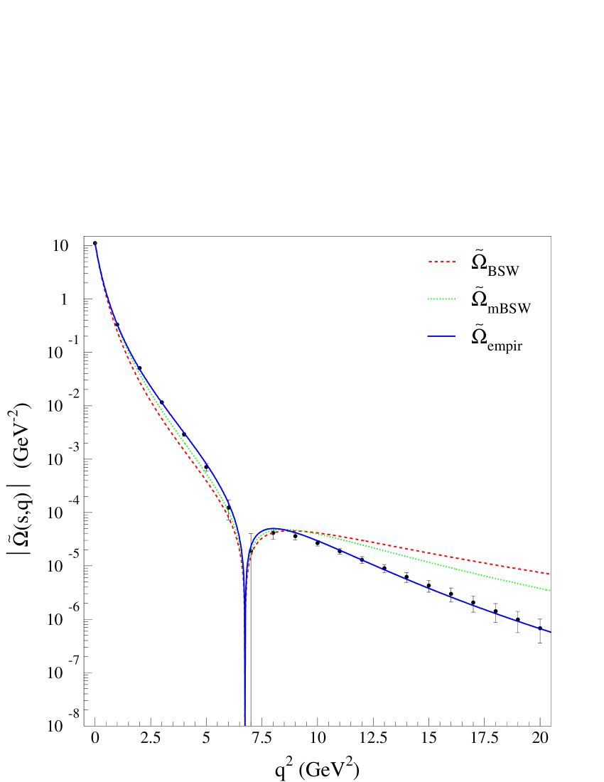
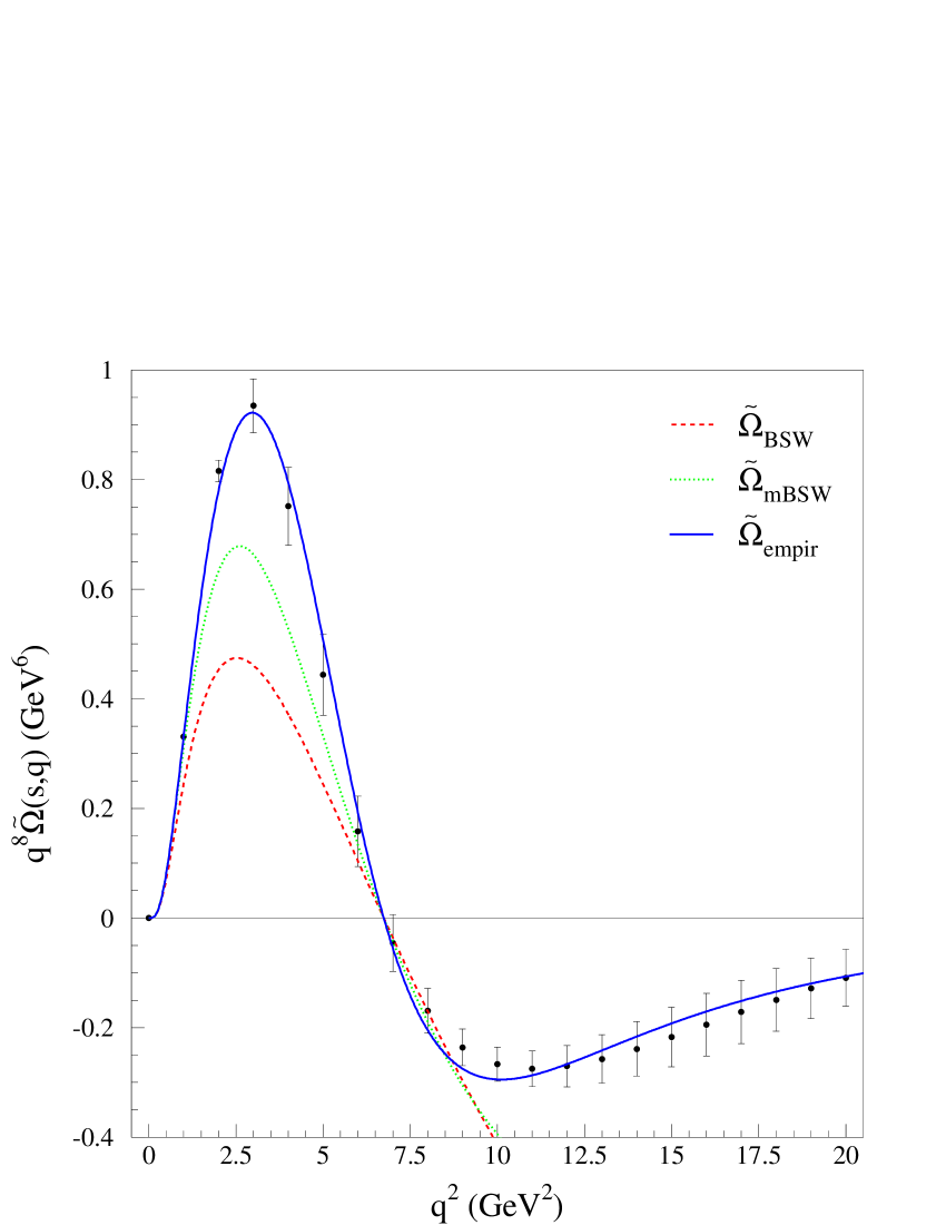
Figure 14: Generated points with uncertainties for the opacity, from the empirical fit to $pp$ scattering data at 52.8 GeV. The curves are the result of the data reduction through $\tilde{\Omega}_{\mathrm{BSW}}(q)$, Eqs. (38) and (39), $\tilde{\Omega}_{\mathrm{mBSW}}(q)$, Eqs. (38) and (40) and $\tilde{\Omega}_{\mathrm{empir}}(q)$, Eq. (44). (Table 8).

We see that, although in both cases the modulus of the opacity is reasonably reproduced up to $q^{2}\sim$ 8 GeV², deviations occur above this region and as a consequence, the $\chi^{2}/DOF$ are too large (Table 8). Moreover, the plot of $q^{8}\tilde{\Omega}(q)$ indicates that both parametrizations do not reach the generated points, except near the fixed position of the zero and near the origin.

However, roughly, the result with $\tilde{\Omega}_{\mathrm{mBSW}}$ is nearer the empirical points then that with the $\tilde{\Omega}_{\mathrm{BSW}}$. This effect is directly related to the square in the $q^{2}/q_{0}^{2}$ term and may also explain the better reproduction of the differential cross section data at large momentum transfers obtained with the multiple diffraction model (compare, for example, the results for $\bar{p}p$ at 546 GeV in bsw03 and mcjp ). Obviously, the position of the zero as obtained in both models, from the phenomenological analysis, Eqs. (33) and (37), is not in agreement with the empirical result.

We have already stressed that our model independent analysis indicates only one possible empirical result and that could explain some of the differences with the parametrizations discussed above. However, even taking into account this limitation, it may be useful, in the phenomenological context, to investigate what kind of analytical parametrization can reproduce the generated points in Fig. 14 and that is our next task here.

$\bullet$ Empirical parametrization for the eikonal

We have tested several analytical parametrizations in order to reproduce the extracted points in Fig. 14. The best result was obtained with an additional square in the $q^{2}/q_{0}^{2}$ term present in the denominator of the $f_{\mathrm{mBSW}}$ function, leading to the following novel empirical (empir) parametrization for the opacity

$$\tilde{\Omega}_{\mathrm{empir}}(q)=\frac{C}{[1+q^{2}/\alpha^{2}]^{2}[1+q^{2}/\beta^{2}]^{2}}\frac{1-q^{2}/q_{0}^{2}}{1+[q^{2}/q_{0}^{2}]^{4}}.$$ (44)

The results of the fit to the extracted points are displayed in Fig. 14 and Table 8 (third colum), showing that the reproduction of the data is quite good. Although this empirical parametrization may play some important role in the phenomenological context, presently, we can not provide a physical interpretation to it. We note, however, that a typical difference among all the above parametrizations concerns the asymptotic behavior, since for $q^{2}\rightarrow\infty$ we have

$$\tilde{\Omega}_{\mathrm{BSW}}(q)\sim-\frac{1}{(q^{2})^{4}},\quad\tilde{\Omega}_{\mathrm{mBSW}}(q)\sim-\frac{1}{(q^{2})^{5}},$$

$$\tilde{\Omega}_{\mathrm{empir}}(q)\sim-\frac{1}{(q^{2})^{7}}.$$

Some other aspects are discussed in the following section.

6.3 Electromagnetic and hadronic form factors

The Wu-Yang conjecture, associating the unknown hadronic matter form factor with electromagnetic form factor wy , has played a fundamental and historical role in the phenomenological context. Also important, as we have recalled, has been the identification of the hadronic form factor with the dipole parametrization, Eq. (28), for the Sachas electric form factor dl . These ideas date back to the end of the sixties and, on the other hand, presently, abundant data on the electromagnetic nucleon form factors are available, at both time-like ($q^{2}<0$) and space-like ($q^{2}>0$) regions, allowing new insights in that old conjecture. Most important to our phenomenological purposes, is the fact that recent experiments have indicated an unexpected decrease in the proton electric form factor, as the momentum transfer increases, not in disagreement with the possibility to reach zero just around $q_{0}^{2}\approx 7.5$ GeV².

Therefore, to finish this work, it may be worthwhile to explore some possible connections between these results from the electromagnetic sector and those concerning the eikonal zero at $q_{0}^{2}\approx$ 7 GeV², presented in the preceding sections (some arguments on this respect have already been discussed in cmm ; mmm ). To this end we first summarize the new information on the proton electric form factor and then discuss possible empirical connections with our results. We shall not go into details, but only quote some results of interest to our discussion. For recent detailed reviews on the subject in both experimental and theoretical contexts, see, for example r1 ; r2 .

6.3.1 Rosenbluth and polarization transfer results

The traditional technique to experimentally investigate the nucleon electromagnetic form factors has been the separation method by Rosenbluth rose , which is based on the measurement of the differential cross section from unpolarized electron-nucleon scattering. For the electron-proton case, the results have indicated a scaling law for the ratio rose1 ; rose2

$$R_{p}=\mu_{p}\frac{G_{E}(q^{2})}{G_{M}(q^{2})}\approx 1,$$

where $\mu_{p}$ is the proton magnetic moment and $G_{E}$, $G_{M}$ the Sachas electric and magnetic form factors.

In 2000 - 2005, experiments with polarized electron beam, in polarization transfer scattering,

$$\vec{e}p\rightarrow e\vec{p},$$

have allowed simultaneous measurements to be made of the transverse and longitudinal components of the recoil proton’s polarization. By means of this polarization transfer technique the ratio $G_{E}/G_{M}$ can be directly determined with great reduction of the systematic uncertainties at large momentum transfers, $q^{2}:4-9$ GeV². The surprising result was the indication that this ratio decreases almost linearly with increasing momentum transfers pt1 ; pt2 ; pt3 , leading even to a parametrization, at large $q^{2}$, of the form pt2

$$R_{p}=1-0.135(q^{2}-0.24),$$

which, by extrapolation, indicates a zero (change of signal) in $G_{E}$ at

$$q_{0}^{2}\approx 7.6\ \mathrm{GeV}^{2}.$$

From a theoretical point of view, radiative corrections associated with two-photon exchange process, have been extensively investigated as possible source of the observed differences. As commented on before, we shall not treat these aspects here; see r1 ; r2 for all the details and references.

6.3.2 The Proton Electric Form Factor

Recently, a global analysis of the world’s data on elastic electron-proton scattering, taking into account the effects of two-photon exchange has been performed. The analysis combines both the corrected Rosenbluth cross section and polarization transfer data, providing the corrected values of $G_{E}$ and $G_{M}$ over the full $q^{2}$ range with available data ffdata . The results for the ratio $G_{E}/G_{D}$ between the proton electric form factor and the dipole parametrization (with $\mu^{2}=0.71$ GeV²), covering the region $q^{2}\approx 10^{-2}-6$ GeV², are displayed in Figs. 15 and 16.

These data clearly show the deviation of $G_{E}$ from $G_{D}$ for $q^{2}$ above $\approx 1$ GeV² and, from a strictly empirical point of view, that $G_{E}$ might reach zero around $q_{0}^{2}\approx$ 7 - 8 GeV². Obviously, this zero might also be reached in an asymptotic process, as predicted, for example, in the Unitary & Analytic model dub .

Anyway, in the context of the Wu-Yang conjecture, it may be worthwhile to compare the parametrizations for the hadronic form factors from eikonal models with one zero (Sect. 6.2.4) and the above data. To this end we return to the following parametrizations for the hadronic proton form factor (Chou-Yang context), with the following notation

$$G_{\mathrm{BSW}}=\frac{1}{[1+q^{2}/\alpha^{2}]}\frac{1}{[1+q^{2}/\beta^{2}]}\sqrt{\frac{1-q^{2}/q_{0}^{2}}{1+q^{2}/q_{0}^{2}}},$$ (45)

$$G_{\mathrm{mBSW}}=\frac{1}{[1+q^{2}/\alpha^{2}]}\frac{1}{[1+q^{2}/\beta^{2}]}\sqrt{\frac{1-q^{2}/q_{0}^{2}}{1+[q^{2}/q_{0}^{2}]^{2}}},$$ (46)

$$G_{\mathrm{empir}}=\frac{1}{[1+q^{2}/\alpha^{2}]}\frac{1}{[1+q^{2}/\beta^{2}]}\sqrt{\frac{1-q^{2}/q_{0}^{2}}{1+[q^{2}/q_{0}^{2}]^{4}}}.$$ (47)

The point is to construct the ratio of each of the above formulas with the dipole parametrization, Eq. (28),

$$\frac{G_{i}(q)}{G_{D}(q)},\quad i=\mathrm{BSW},\ \mathrm{mBSW},\ \mathrm{empir}$$ (48)

and perform the fits to the data in Fig. 15 through the code CERN-minuit. In addition we consider two variants for the data reduction:

#1.

$q_{0}^{2}$ fixed to our average result in the ISR region, Eq. (21), $q_{0}^{2}$ = 7.0 GeV² and $\alpha^{2}$ and $\beta^{2}$ as free fit parameters.

#2.

$q_{0}^{2}$ as a free fit parameter together with $\alpha^{2}$ and $\beta^{2}$.

The results are shown in Figs. 15 and 16, respectively and the numerical results are displayed in Table 9.

Table 9: Results of the fit to the extracted ratio between the proton electric form factor and dipole parametrization. All the parameters in GeV².

$q_{0}^{2}$		BSW	mBSW	empir
		Eq. (45) and (48)	Eq. (46) and (48)	Eq. (47) and (48)
	$\alpha^{2}$	1.550 $\pm$ 0.073	1.310 $\pm$ 0.064	1.156 $\pm$ 0.055
7 GeV2	$\beta^{2}$	0.437 $\pm$ 0.010	0.446 $\pm$ 0.012	0.474 $\pm$ 0.014
	$\chi^{2}/DOF$	1.36	1.34	1.79
	$\alpha^{2}$	1.8068 $\pm$ 0.097	1.508 $\pm$ 0.084	1.328 $\pm$ 0.070
free	$\beta^{2}$	0.4192 $\pm$ 0.0090	0.423 $\pm$ 0.011	0.446 $\pm$ 0.012
	$q_{0}^{2}$	6.06 $\pm$ 0.11	6.12 $\pm$ 0.13	6.04 $\pm$ 0.10
	$\chi^{2}/DOF$	1.11	1.11	1.41

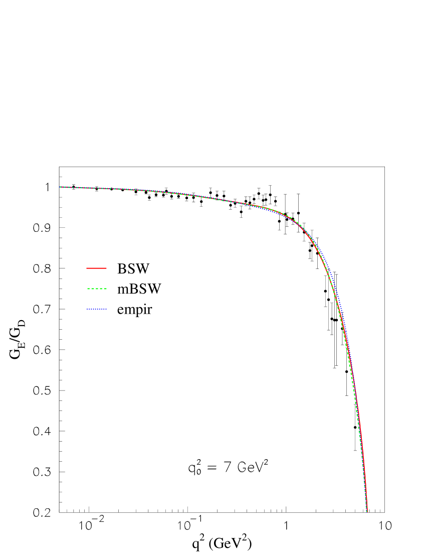
Figure 15: Experimental data on the ratio of the proton electric form factor to the dipole parametrization, $G_{E}/G_{D}$ from ffdata and fit results through BSW, mBSW and the empirical parametrizations, Eqs. (45), (46) and (47), respectively and Eq. (48), with $q_{0}^{2}$ = 7 GeV² (Table 9).

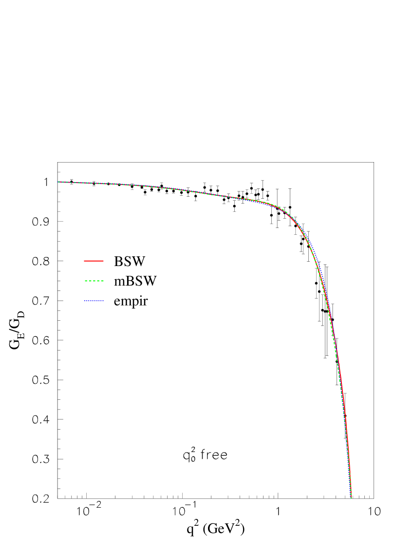
Figure 16: Same as Fig. 15 with $q_{0}^{2}$ as a free fit parameter.

We see that, although all the parametrizations provide good visual descriptions of the data, the best statistical results have been obtained with $G_{\mathrm{BSW}}$, Eq. (45) and $G_{\mathrm{mBSW}}$, Eq. (46) and $q_{0}^{2}$ as a free fit parameter: $\chi^{2}/DOF$ = 1.11 in both cases. Moreover, both fits indicate $q_{0}^{2}\approx$ 6.1 GeV², a value barely compatible with our average estimation, Eq. (21). The statistical results with $G_{\mathrm{empir}}$, Eq. (47), are not so good since the $\chi^{2}/DOF$ is higher.

These results suggest that parametrizations (45-47) have correlations with the recent global analysis on the proton electric form factor ffdata , a fact that may bring about new theoretical insights in the phenomenological context. It seems to us that a striking aspect of the above empirical results is the fact that they corroborate the old Wu-Yang conjecture and just after a complete change in the experimental knowledge on the electromagnetic form factors along the years (Rosenbluth scaling versus polarization transfer results).

7 Summary and final remarks

We have developed an empirical analysis of the differential cross section data on elastic $pp$ scattering in the region 19.4 $\leq\sqrt{s}\leq$ 62.5 GeV. The analysis introduces two main improvements if compared with a previous one cmm ; cm , the first associated with the structure of the parametrization and the second with the selected data ensemble. We have also presented a critical discussion of the experimental data available, checking, in some detail, that data at large momentum transfers ($q^{2}>$ 3.5 GeV²) do not depend on the energy in the particular region 23.5 $\leq\sqrt{s}\leq$ 62.5 GeV. Based on this information, we have included the data obtained at 27.4 GeV only in the 5 sets in the above energy region and not at 19.4 GeV, as done in cmm . With these improvements we have obtained better statistical results then in previous analysis cmm ; cm .

As commented on at the beginning of Sect. 6, these fits represent only one solution. In fact, the data reduction of the differential cross sections with $\sim$ 150 $DOF$ and $\sim$ 10 free parameters is a very complex process and the main point is the lack of information on the contributions from the real and imaginary parts of the amplitude beyond the forward direction, leading to an infinity number of possible solutions. To our knowledge, the only model independent information on the real part at $q^{2}>$ 0 concerns a theorem by Martin, which indicates a change of signal (zero) at small values of the momentum transfer martin . The exact position, however, can not be inferred. In our approach, by including in the parametrization the experimental results on $\sigma_{\mathrm{tot}}$ and $\rho$ at each energy, we correctly reproduce the forward behavior in the region investigated. The zero in the real part is generated by using two equal exponential contributions (in $q^{2}$) in both real and imaginary parts ($m=2$ and $n=4,5$ and $6$ in Eq. (11)). However, the zero can also be generated without this constraint sma .

Therefore, a general and detailed analysis on the physically acceptable data reductions, constrained by model independent formal results, is necessary and we are presently investigating the subject sma . Anyway, despite the above limitations in the present analysis, it allows us to infer several novel qualitative and some quantitative results, as summarized in what follows.

With the data reduction and by means of the semi-analytical method, the imaginary part of the eikonal (real opacity function), in the momentum transfer space, has been extracted, together with uncertainty regions from error propagation. That was achieved within approximation (16), justified by the fit results. Although the method provides model independent results for the eikonal in both $q$ and $b$ spaces, we focused here only the question of the eikonal zero in $q$ space. Different from the previous analysis cmm , we obtained statistical evidence for a change of sign in the imaginary part of the eikonal only in the region 23.5 $\leq\sqrt{s}\leq$ 62.5 GeV and not at 19.4 GeV. Moreover, the position of the zero in this energy region is approximately constant with average value $q_{0}^{2}=$ 7 $\pm$ 1 GeV², compatible with the result obtained in cm , where only the ISR data was considered.

The implication of the eikonal zero in the phenomenological context has been also discussed in some detail. We have shown that models with two dynamical contributions for the imaginary part of the eikonal (positive at small and negative at large momentum transfers) allows good descriptions of the differential cross section data in the full $q^{2}$ region with available data. In this context the BSW model play a central role due to both its theoretical basis and the reproduction of the experimental data. We have also discussed some analytical parametrizations for the extracted eikonal, either from phenomenological models ($\Omega_{\mathrm{BSW}}$ and $\Omega_{\mathrm{mBSW}}$) or by introducting a novel form ($\Omega_{\mathrm{empir}}$).

Connections between the extracted eikonal and recent global analysis on the proton electric form factor have also been discussed. In particular we have shown that eikonal models presenting good descriptions of the elastic hadron scattering, make use of effective form factors also compatible with the proton electric form factor and in this case, the fits have indicated a zero at $q_{0}^{2}\approx$ 6.1 GeV². This compatibility between hadronic and electric form factors seems a remarkable fact if we consider all the theoretical and experimental developments that took place after the original conjecture by Wu and Yang.

We understand that all these empirical results can provide novel and important insights in the phenomenological context, since, through the Fourier transform, suitable inputs for the “unknown” impact parameter contribution can be obtained. For example, in the case of QCD-inspired models, the factorization in $s$ and $b$ at the elementary level (Sect. 6.2.1) allows, in principle, any choice for the impact parameter contribution without losing the semi-hard QCD connections ($\sigma_{gg}(s)$, for example). The use of parametrizations (45-47) in the place of the dipole parametrization at the elementary level ($qq$, $qg$, $gg$ contributions) may be much more efficient in the description of the differential cross section data at large values of the momentum transfer. That is, at least, what our phenomenological analysis suggests. We are presently investigating this subject.

Finally we would like to call attention to a central aspect related to the importance of the differential cross section information at large momentum transfers in any reliable model independent analysis. Comparison of Figs. 9 and 10 shows clearly that the lack of data at large momentum transfers turns out to make very difficult or even impossible, any detailed knowledge of the elastic scattering processes. Despite the technical difficulties in performing experiments at a large momentum region, we think this should be an aspect to be taken into account in the forthcoming experiments. We end this work stressing once more the assertion by Kawasaki, Maehara and Yonezawa kmy “Such experiments will give much more valuable information for the diffraction interaction rather than to go to higher energies”.

- (1) F. Gelis, T. Lappi, R. Venugopalan, Int. J. Mod. Phys. E 16, 2595 (2007)
- (2) V. Barone and E. Predazzi, High-Energy Particle Diffraction (Spring-Verlag, Berlin, 2002)
- (3) S. Donnachie, G. Dosch, P.V. Landshoff, O. Natchmann, “Pomeron Physics and QCD”, (Cambridge University Press, 2002)
- (4) P.A.S. Carvalho, A.F. Martini, M.J. Menon, Eur. Phys. J. C 39, 359 (2005)
- (5) P.A.S. Carvalho, M.J. Menon, Phys. Rev. D 56 7321 (1997)
- (6) R.F. Ávila, A.F. Martini, M.J. Menon, Relatório da XVII Reunião de Trabalho sobre Interações Hadrônicas, edited by F.S. Navarra, F.O. Durães, Y. Hama (Instituto de Física, Universidade de São Paulo, São Paulo, 2005) pp. 52 - 56.
- (7) pp2pp Collaboration, www.rhic.bnl.gov/pp2pp
- (8) TOTEM Collaboration, http://totem.web.cern.ch/Totem/
- (9) J. R. Cudell, E. Martynov, O. Selyugin, A. Lengyel, Phys. Lett. B 587, 78 (2004).
- (10) J.R. Cudell, A. Lengyel, E. Martynov, Phys. Rev. D 73, 034008 (2006)
- (11) S. Bültmann et al. Phys. Lett. B 579, 245 (2004)
- (12) U. Amaldi and K. R. Schubert, Nucl. Phys. B 166, 301 (1980)
- (13) K.R. Schubert, Landolt-Börnstein, Numerical Data and Functional Relationships in Science and Technology, New Series, Vol. I/9a (Springer-Verlag, Berlin, 1979)
- (14) A. S. Carrol et al. Phys. Lett. B 80, 423 (1979)
- (15) L. A. Fajardo et al., Phys. Rev. D 24, 46 (1981)
- (16) U. Amaldi et al., Phys. Lett. B 43, 231 (1973)
- (17) U. Amaldi et al., Phys. Lett. B 66, 390 (1977)
- (18) C.W. Akerlof et al., Phys. Rev. D 14, 2864 (1976)
- (19) W. Faissler et al. Phys. Rev. D 23, 33 (1981)
- (20) G. Fidecaro et al., Phys. Lett. B 105, 309 (1981)
- (21) R. Rubinstein et al., Phys. Rev. D 30, 1413 (1984)
- (22) H. De Kerret et al., Phys. Lett. B 68, 374 (1977)
- (23) E. Nagy et al. Nucl. Phys. B 150, 221 (1979)
- (24) A. Donnachie, P.V. Landshoff, Z. Phys. C 2, 55 (1979); Phys. Lett. B 123, 345 (1983); Phys. Lett. B 387, 637 (1996)
- (25) F. James, MINUIT - Function Minimization and Error Analysis (CERN, 2002)
- (26) A. Martin, Phys. Lett. B 404, 137 (1997)
- (27) M. Kawasaki, T. Maehara, M. Yonezawa, Phys. Rev. D 67, 014013 (2003)
- (28) T.T. Wu, C.N. Yang, Phys. Rev. 137B, 708 (1965)
- (29) N. Byers, C.N. Yang, Phys. Rev. 142, 976 (1966)
- (30) L. Durand, R. Lipes, Phys. Rev. Lett. 20, 637 (1968)
- (31) T.T. Chou and C.N. Yang, in High Energy Physics and Nuclear Structure, edited by G. Alexander (North-Holland, Amsterdam, 1967) p. 348; Phys. Rev. 170, 1951 (1968); Phys. Rev. Lett. 20, 1213 (1968); Phys. Rev. 175, 1832 (1968)
- (32) T.T. Chou and C.N. Yang, Phys. Rev. Lett. B 244 113 (1990)
- (33) M.M. Block, E.M. Gregores, F. Halzen, G. Pancheri, Phys. Rev. D 58, 017503 (1998); 60, 054024 (1999)
- (34) E.G.S. Luna, A.F. Martini, M.J. Menon, A. Mihara, A.A. Natale, Phys. Rev. D 72, 034019 (2005)
- (35) R.J. Glauber, J. Velasco, Phys. Lett. B 147, 380 (1984)
- (36) R.J. Glauber, J. Velasco, in Proceedings of the Second International Conference on Elastic and Diffractive Scattering, edited by K. Goulianos (Editions Frontieres, Gif-sur-Yvette Cedex, France, 1988) p. 219
- (37) R.J. Glauber, in Lectures in Theoretical Physics, edited by W. E. Brittin et al. (Interscience, New York, 1959) Vol. I, p.315; W. Czyż and L.C. Maximon, Ann. Phys. (N.Y.) 52, 59 (1969); V. Franco and G.K. Varma, Phys. Rev. C 18, 349 (1978).
- (38) C. Bourrely, J. Soffer and T.T. Wu, Phys. Rev. D 19, 3249 (1979); Nucl. Phys. B247, 15 (1984); Phys. Rev. Lett. 54, 757 (1985);
- (39) C. Bourrely, J. Soffer, T. T. Wu, Eur. Phys. J. C 28, 97 (2003)
- (40) M.J. Menon, Doctoral Thesis, Instituto de Física Gleb Wataghin, Universidade Estadual de Campinas, 1988
- (41) J. Bellandi, R.J.M. Covolan, M.J. Menon, B.M. Pimentel, Hadronic J. 11, 17 (1988)
- (42) M.J. Menon, Phys. Rev. D 48, 2007 (1993); A.F. Martini, M.J. Menon, D.S. Thober, Phys. Rev. D 54, 2385 (1996)
- (43) M.J. Menon, Nucl. Phys. B (Proc. Suppl.) 25, 94 (1992)
- (44) M.J. Menon, Canadian J. Phys. 74, 594 (1996)
- (45) A.F. Martini, M.J. Menon, Phys. Rev. D 56, 4338 (1997)
- (46) R.J.M. Covolan, L.L. Jenkovszky, E. Predazzi, Z. Phys. C, 51, 459 (1991); R.J.M. Covolan, P. Desgrolard, M. Giffon, L.L. Jenkovszky, E. Predazzi, Z. Phys. C 58, 109 (1993).
- (47) A.F. Martini, M.J. Menon, J. Montanha, in IX Hadron Physics and VII Relativistic Aspects of Nuclear Physics, edited by M.E. Bracco et al., AIP Conference Proceedins V. 739 (American Institute of Physics, New York, 2004) p. 578
- (48) C.F. Perdrisat, V. Punjabi, M. Vanderhaeghen, hep-ph/0612014
- (49) C.E. Carlson, M. Vanderhaeghen, hep-ph/0701272
- (50) M.N. Rosenbluth, Phys. Rev. 79, 615 (1950)
- (51) R.C. Walker et al. Phys. Rev. D 49, 5671 (1994); L. Andivahis et al., Phys. Rev. D 50, 5491 (1994)
- (52) J. Arrington, Phys. Rev. C 68, 034325 (2003); M.E. Christy et al., Phys. Rev. C 70, 015206 (2004); I.A. Qattan et al., Phys. Rev. Lett. 94, 142301 (2005), nucl-ex/0410010
- (53) M. K. Jones et al., Phys. Rev. Lett. 84, 0398 (2000); O. Gayou et al. Phys. Rev. C 64, 138202 (2001)
- (54) O. Gayou et al. Phys. Rev. Lett 88, 092301 (2002)
- (55) V. Punjabi et al., Phys. Rev. C 71, 055202 (2005) [Erratum-ibid C 71, 069902 (2005)]
- (56) J. Arrington, W. Melnitchouk, J.A. Tjon, 0707.1861 [nucl-ex]
- (57) A.Z. Dubnic̃ková, S. Dubnička, 0708.0162 [hep-ph]
- (58) G.L.P. Silva, M.J. Menon, R.F. Ávila, Int. J. Mod. Phys. E 16, 2923 (2007)