Effective motion of a virus trafficking inside a biological cell

Abstract

Virus trafficking is fundamental for infection success and plasmid cytosolic trafficking is a key step of gene delivery. Based on the main physical properties of the cellular transport machinery such as microtubules, motor proteins, our goal here is to derive a mathematical model to study cytoplasmic trafficking. Because experimental results reveal that both active and passive movement are necessary for a virus to reach the cell nucleus, by taking into account the complex interactions of the virus with the microtubules, we derive here an estimate of the mean time a virus reaches the nucleus. In particular, we present a mathematical procedure in which the complex viral movement, oscillating between pure diffusion and a deterministic movement along microtubules, can be approximated by a steady state stochastic equation with a constant effective drift. An explicit expression for the drift amplitude is given as a function of the real drift, the density of microtubules and other physical parameters. The present approach can be used to model viral trafficking inside the cytoplasm, which is a fundamental step of viral infection, leading to viral replication and in some cases to cell damage.

1 Introduction

Because cytosolic transport has been identified as a critical barrier for synthetic gene delivery [1], plasmids or viral DNAs delivery from the cell membrane to the nuclear pores has attracted the attention of many biologists. The cell cytosol contains many types of organelles, actin filaments, microtubules and many others, so that to reach the nucleus, a viral DNA has to travel through a crowded and risky environment. We are interested here in studying the efficiency of the delivery process and we present a mathematical model of virus trafficking inside the cell cytoplasm. We model the viral movement as a Brownian motion. However, the density of actin filaments and microtubules, inside the cell, can hinder diffusion, as demonstrated experimentally [2]. In a crowded environment, we will model the virus as a material point. This reduction is simplistic for several reasons: actin filament network can trapped a diffusing object and beyond a certain size, as observed experimentally, a DNA fragment cannot find its way across the actin filaments [2]. Active directional transport along microtubules or actin filaments seems then the only way to deliver a plasmid to the nucleus. The active transport of the virus involves in general motor proteins, such as Kinesin (to travel in the direction of the cell membrane) or Dynein (to travel toward the nucleus). Once a virus is attached to a Dynein protein, its movement can be modeled as a deterministic drift toward the nucleus.

Recently, a macroscopic modeling has been developed to describe the dynamics of adenovirus concentration inside the cell cytoplasm [3]. This approach offers very interesting results about the effect of microtubules, but neglects the complexity of the geometry and cannot be used to describe the movement of a single virus, which might be enough to cause cellular infection. Modeling a virus trafficking imposes to use a stochastic description. We model here the motion of a virus as that of a material point, so the probability of its trapping by actin filaments or microtubules is neglected. In the present approximation, the viral movement has two main components: a Brownian one, which accounts for its free movement, and a drift directed towards the centrosome or MTOC (Microtubules Organization Center), an organelle located near the nucleus. The magnitude of the drift along microtubules depends on many parameters, such as the binding and unbinding rates and the velocity of the motor proteins [4].

In the present approach, we present a method to approximate a time dependent dynamics of virus trafficking by an effective stochastic equation with a radial steady state drift. The main difficulties we have to overcome arise from the time dependent nature of the trajectories which consists of intermittent epochs of drifts and free diffusion. We propose to derive an explicit expression for the steady state drift amplitude. In this approximation, the effective drift will gather the mean properties of the cytoplasmic organization such as the density of microtubules and its off binding rate.

Our method to find the effective drift can be described as follow: first, we approximate the cell geometry as a two dimensional disk and use a pure Brownian description to approximate the virus diffusion step. This geometrical approximation is valid, for any two dimensional cell such as the in vitro flat skin fibroblast culture cells [3]: indeed, due to their adhesion to the substrate, the thickness of these cells can be neglected in first approximation. Second, when the distribution of the initial viral position is uniform on the cell surface, we will estimate, during the diffusing period, the hitting position on a microtubule. By solving a partial differential equation, inside a sliced shape domain, delimited by two neighboring microtubules, we will provide an estimate of the mean time to the most likely hitting point. Finally, the amplitude of the radial steady state drift will be obtained by an iterative method which assumes that, after a virus has moved a certain distance along a microtubule, it is released at a point uniformly distributed on the final radial distance from the nucleus, ready for a new random walk. This scenario repeats until the virus reaches the nucleus surface. Finally, we will compute the mean time, the mean number of steps before a virus reaches the nucleus and the amplitude of the effective drift by using the following criteria: the Mean First Passage Time (MFPT) to the nucleus of the iterative approximation is equal to the MFPT obtained by solving directly an Ornstein-Uhlenbeck stochastic equation. The explicit computation of the effective drift is a key result in the estimation of the probability and the mean time a single virus or DNA molecule takes to reach a small nuclear pore [5].

2 Modeling stochastic viral movement inside a biological cell

We approximate the cell as a two dimensional geometrical domain $\Omega$, which is here a disk of radius R and the nucleus located inside is a concentric disk of much smaller radius $\delta<<R$. We model the motion of an unattached DNA fragment as a material point, so that the probability of its trapping by actin filaments or microtubules is neglected. The motion of a (DNA) molecule of mass $m$ is described by the overdamped limit of the Langevin equation (Smoluchowski’s limit) [6] for the position $\mathbf{X}(t)$ of the molecule at time $t$. When the particle is not bound to a microtubule filament, its movement is described as pure Brownian with a diffusion constant $D$. When the particle hits a filament, it binds for a certain random time and moves along with a determinist drift. We only take into account the movement toward the nucleus, which is confound here with the MTOC (Microtubule organization center), an organelle where all microtubules converge (see figure (1)). For $\delta<|\mathbf{X}(t)|<R$, we describe the overall movement by the stochastic rule

$$\mathbf{\dot{X}}=\left\{\begin{array}[]{l}\sqrt{2D}\mathbf{\dot{w}}\quad\mbox{ for }\quad\mathbf{X}\left(t\right)\quad\mbox{ free }\\ \\ V\frac{\mathbf{r}}{|\mathbf{r}|}\quad\mbox{ for }\quad\mathbf{X}\left(t\right)\quad\mbox{ bound }\end{array}\right.$$ (4)

where $V$ is a constant velocity, $\mathbf{\dot{w}}$ a $\delta$-correlated standard white noise and $\mathbf{r}$ the $\mathbf{X}$ radial coordinate, the origin of which is the center of the cell. We assume that all filaments starting from the cell surface end on the nucleus surface. The binding time corresponds to a chemical reaction event and we assume that it is exponentially distributed and for simplicity we approximate it by a constant $t_{m}$.

Once a virus enters the cell membrane, its moves according to the rule (4), until it hits a nuclear pore. Although nuclear pores occupy a small portion of the nuclear surface, we only consider the virus movement until it hits the nuclear surface $D\left(\delta\right)$. In this article, our goal is to replace equation (4) by a steady state stochastic equation

$$\dot{\bf X}=\mathbf{b}(\mathbf{X})+\sqrt{2D}\mathbf{\dot{w}},$$ (5)

where the drift $\mathbf{b}$ is radially symmetric. In a first approximation, we consider a constant radial drift $\mathbf{b}(\mathbf{X})=-B\frac{\mathbf{r}}{|\mathbf{r}|}$ and compute hereafter the value of the constant amplitude $B$ such that the MFPT of the process (5) and (4) to the nucleus are equal.

 

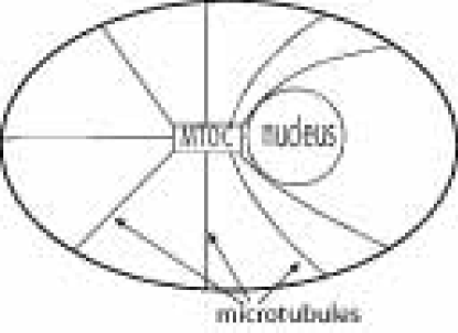
Fig. 1: Cell geometry. (a) Cell’s microtubules network. All microtubules starting from the cell membrane converge to the Microtubule Organization center (MTOC), located near the nucleus. (b) simplified cell’s microtubules network organization. The MTOC coincides with the nucleus.

2.1 Modeling viral dynamics in the cytoplasm

Inside the cytosol, microtubules are distributed on the cell surface and converging radially to the MTOC. We denote by $\rho$ this distribution (see figure (1)). We do not take into account in the present analysis, the effect of organelle crowding due to the endoplasmic reticulum, the Golgi apparatus and many others. However, it is always possible to include them indirectly by using an apparent diffusion constant. We consider the fundamental domain $\tilde{\Omega}$ defined as the two dimensional slice of angle $\Theta$ between two neighboring microtubules. We consider here that microtubules are uniformly distributed and thus $\Theta=\frac{2\pi}{N}$, where $N$ is the total number of microtubules.

Although a virus can drift along microtubules in both directions by using dynein (resp. kinesin) motor proteins for the inward (resp. forward) movement, we only take into account the drift toward the nucleus [7]. It is still unclear what is the precise mechanism used by a virus to select a direction of motion. Attached to a dynein molecule, the virus transport consists in several steps of few nanometers: the length of each step depends on the load of the transported cargo and ATP-concentration [8]. We neglect here the complexity of this process, assuming that ATP molecules are abundant, uniformly distributed over the cell and is not a limiting factor. We thus assume the bound particle moves towards the nucleus with the mean constant velocity $V$. When the particle is released away from the microtubule, inside the domain, the process can start afresh and the particle diffuses freely. Because the Smoluchowski limit of the Langevin equation does not account for the change in velocity, we release the the particle at a certain distance away from the microtubule, but at a fixed distance from the nucleus (at an angle chosen uniformly distributed), see figure 2.

Because microtubules are taken uniformly distributed, we can always release the virus inside the slice $\tilde{\Omega}$, between two neighboring microtubules. Thus the movement of the virus will be studied in $\tilde{\Omega}$: inside the cytosol, the viral movement is purely Brownian until it hits a microtubule which is now the lateral boundary of $\tilde{\Omega}$ (see figure (2)). We assume that once a virus hits a microtubule, with probability one, the dynamics switches from diffusion to a determinist motion with a constant drift. A virus spends on a microtubule a time that we consider to be exponentially distributed, since this time is the sum of escape time from deep potential wells. We approximate the total time on a microtubule by the mean time $t_{m}$. Thus a virus moves to a distance $d_{m}=Vt_{m}$ along microtubule, which depends only on the characteristic of the virus-microtubule interactions. To summarize, the virus trajectory is a succession of diffusion steps mixed with some periods of attaching and detaching to microtubules. Thus scenario repeats until the virus hits the nucleus surface (Figure (2)).

   

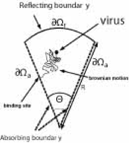
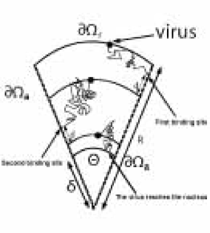
Fig. 2: Virus trafficking inside a cell. (a) Representation of the cell portion between two microtubules. (b) Transport along microtubules: Two fundamental steps are represented. A fundamental step is made of the two intermediate step which are first the diffusion inside the domain followed by the directed motion along the microtubule.

2.2 Computing the MFPT to reach the nucleus

We define the mean time to infection as the MFPT a virus reaches the surface of the disk $D\left(\delta\right)$ inside the domain $\tilde{\Omega}$ (see figure (2)).

To estimate the mean time to infection, we note that we can decompose the overall motion as a repeated fundamental step. This step consists of the free diffusion of the particle inside the domain followed by the motion along the microtubule. The total time of infection $\tau_{i}$ is then the sum of times the particle spends in each step. Although the time on microtubule is determinist equal to $t_{m}$, the diffusing time is not easy to compute and depend on the initial condition. Ultimately $\tau_{i}$ depends on the number of times the fundamental step repeats before the particle reaches the nucleus.

Let us now described each step: the first step starts when the virus enter the cell at the periphery $r=R=R_{0}$ (at a random angle $\theta\in[0;\Theta]$) and ends when the virus hits either the lateral boundary or the nucleus. We now consider the first passage time ${u}\left(R_{0}\right)$ to the absorbing boundary and by $r(R_{0})$ the hitting position. To account for the determinist drift, we move during a deterministic time $t_{m}$ the virus from a distance $d_{m}$ along the microtubule. In that case, the initial random position for the next step is given by $r=R_{1}=r(R_{0})-d_{m}$ and the total time in step $1$ is ${u}\left(R_{0}\right)+t_{m}.$

We iterate the process as follow and consider in each step k the distance $R_{k}=r(R_{k-1})-d_{m}$ from which the particle starts and the time ${u}\left(R_{k}\right)+t_{m}$ it spends inside the step. If we denote by $n_{s}$ the random number of steps necessary to reach the nucleus $r=\delta$, the time to infection $\tau_{i}$ is given by

$$\tau_{i}=\sum_{k=0}^{n_{s}-1}{u}(R_{k})+n_{s}t_{m}+t_{r}\hbox{ ,}$$ (6)

where $t_{r}$ is a residual time, which is the time to reach the nucleus before a full step is completed.

We are interested in the estimating the mean first passage MFPT $\tau$ of $\tau_{i}$, given by

$$\tau=E(\tau_{i})=E\displaystyle\left(\sum_{k=0}^{n_{s}-1}{u}(R_{k})\right)+<n_{s}>t_{m}+<t_{r}>,$$ (7)

where $<n_{s}>$ is the mean number of steps and $<t_{r}>$ is the mean residual time. If we introduce the probability density function $p_{m}=Pr\{n_{s}=m\}$ that the number of step is exactly equal to m, we can write

$$\tau=E(\tau_{i})=\sum_{m=1}^{\infty}E\displaystyle\left(\sum_{k=0}^{n_{s}-1}{u}(R_{k})|n_{s}=m\right)p_{m}+<n_{s}>t_{m}+<t_{r}>,$$ (8)

To estimate the MFPT $\tau$, we shall approximate the previous sum by using the mean first passage time $\bar{u}(R_{k})$ in each step $k$. To estimate $\bar{u}(R_{k})$, we will solve (in the next paragraph) the Dynkin’s equation with the following boundary conditions: inside $\tilde{\Omega}$, the particle is reflected at the periphery $r=R$, absorbed at the nucleus $\partial\tilde{\Omega}_{a}$ and at $\theta=0$ and $\theta=\Theta$. We will also estimate the mean distance $\bar{d}_{k}$ covered during step $k$. For that purpose we will estimate the mean exit position $r_{m}(R_{k})$, conditioned on the initial position $r=R_{k}$. Indeed, we will thus get $\bar{d}_{k}=R_{k}-r_{m}(R_{k})-d_{m}$. The estimates of the mean distances covered for each fundamental step will ultimately lead to an approximation of the mean number of step $n=<n_{s}>$: $n$ will be computed such that $R_{n}\geq\delta$ and $R_{n+1}<\delta$ (where $R_{n}=r_{m}(R_{n-1})-d_{m}$ is defined recursively). Finally, we will obtain the following approximation for the infection time

$$\tau\approx\displaystyle{\sum_{k=0}^{n-1}\bar{u}(R_{k})+nt_{m}+<t_{r}>,}$$ (9)

The mean residual time $<t_{r}>$ can be equal either to $\bar{u}(R_{n})+\alpha t_{m},$ where $0\leq\alpha<1$ if the virus binds to a microtubule in the last step and travels a distance $\alpha d_{m}$ on the microtubule, or to the MFPT to the nuclear boundary if $r_{m}(R_{n})<\delta$.

3 Mean First Passage Time and Exit point distribution

In first approximation, under the assumptions of a sufficiently small radius $\delta<<R$ and an angle $\Theta<<1$ , for the computation of the MFPT and the distribution of exit points, we neglect the nuclear area. We define the full pie wedge $\Omega^{R}$ domain of angle $\Theta$. Inside $\Omega^{R}$, we use the boundary conditions described above. Consequently, the MFPT to a microtubule $u=u\left(r,\theta\right)$ of a virus starting initially at position $\left(r,\theta\right)$ is solution of the Dynkin’s equations [6]

$$\displaystyle{D\Delta u\left(\mbox{\boldmath$x$}\right)} = -1\hbox{ for }\mbox{\boldmath$x$}\in\Omega^{R}$$ (10)

$$u\left(\mbox{\boldmath$x$}\right) = 0\hbox{ for }\mbox{\boldmath$x$}\in\partial\Omega^{R}_{a}$$

$$\frac{\partial u}{\partial\mbox{\boldmath$n$}} = 0\hbox{ for }\mbox{\boldmath$x$}\in\partial\Omega^{R}_{r}\hbox{ ,}$$

where $\partial\Omega^{R}_{a}=\{\theta=0\}\cup\{\theta=\Theta\}$ and $\Omega^{R}_{r}=\{r=R\}$.

3.1 The general solution for the MFPT

In this paragraph only we reparametrize the domain by $-\Theta/2\leq\theta\leq\Theta/2$. By writing equation (10) in polar coordinates and using the separation of variables, the general solution of equation

$$\left(\frac{\partial^{2}u}{\partial r^{2}}+\frac{1}{r}\frac{\partial u}{\partial r}+\frac{1}{r^{2}}\frac{\partial^{2}u}{\partial\theta^{2}}\right)\left(r,\theta\right) = -1\hbox{ for }\left(r,\theta\right)\in\Omega^{R}$$ (11)

$$u\left(r,\theta\right) = 0\hbox{ for }\left(r,\theta\right)\in\partial\Omega^{R}_{a}\hbox{}.$$ (12)

is given by [9]

$$u\left(r,\theta\right)=\frac{r^{2}}{4D}\left(\frac{cos\left(2\theta\right)}{cos\left(\Theta\right)}-1\right)+\sum_{n=0}^{\infty}A_{n}r^{\lambda_{n}}cos\left(\lambda_{n}\theta\right),\hbox{ for }-\Theta/2\leq\theta\leq\Theta/2$$ (13)

where the edge boundary is here located at position $\theta=\pm\Theta/2$. The sum in the right-hand side is the general solution of the homogeneous problem $\Delta u=0$ in $\Omega^{R}$. The boundary conditions on the sides of the wedge impose that

$$\lambda_{n}=\left(2n+1\right)\frac{\pi}{\Theta},$$ (14)

while the reflecting condition for $r=R$ reads

$$\frac{\partial u}{\partial r}\left(R,\theta\right)=0\hbox{ for all }\theta\in[-\Theta/2,\Theta/2].$$ (15)

Using the uniqueness of Fourrier decomposition and the boundary condition (15), we obtain that

$$A_{n}=\frac{\left(-1\right)^{n+1}8R^{2-\lambda_{n}}}{D\Theta\lambda_{n}^{2}\left(\lambda_{n}^{2}-4\right)}.$$ (16)

By averaging formula (13) over an initial uniform distribution, the MFPT to a one of the wedge is given by

$$\bar{u}\left(r\right)=\frac{1}{\Theta}\int_{\theta=0}^{\theta=\Theta}u\left(r,\theta\right)d\theta=\frac{r^{2}}{4D}\left(\frac{tan\left(\Theta\right)}{\Theta}-1\right)-\sum_{n=0}^{\infty}\frac{16R^{2-\lambda_{n}}r^{\lambda_{n}}}{D\Theta^{2}\lambda_{n}^{3}\left(\lambda_{n}^{2}-4\right)},$$ (17)

where $\lambda_{n}=\left(2n+1\right)\frac{\pi}{\Theta}$. For $\Theta$ small, equation (17) can be approximated by

$${\bar{u}\left(r\right)=\frac{r^{2}}{4D}\left(\frac{tan\left(\Theta\right)}{\Theta}-1\right)-\frac{16\Theta R^{2}\left(\frac{r}{R}\right)^{\pi/\Theta}}{D\pi^{3}\left(\left(\pi/\Theta\right)^{2}-4\right)}}.$$ (18)

3.2 Exit points distribution

To estimate the position a virus will attach preferentially to the microtubule, we determine the distribution of exit points, when the viral particle initially started at a radial distance from the nucleus. We recall that the probability density function (pdf) $p\left(\mathbf{r},t|\mathbf{r_{0}}\right)$ to find a diffusing particle in a volume element $d\mathbf{r}$ at time t inside the wedge $\tilde{\Omega}$, conditioned on the initial position $\mathbf{r}=\mathbf{r_{0}}$ is solution of the diffusion equation

$$\frac{\partial p\left(\mathbf{r},t|\mathbf{r_{0}}\right)}{\partial t} = D\Delta p\left(\mathbf{r},t|\mathbf{r_{0}}\right)\hbox{ for }\mathbf{r}\in\Omega^{R}$$

$$p\left(\mathbf{r},t|\mathbf{r_{0}}\right) = 0\hbox{ for }\mathbf{r}\in\partial\Omega^{R}_{a}$$

$$\frac{\partial p\left(\mathbf{r},t|\mathbf{r_{0}}\right)}{\partial n} = 0\hbox{ for }\mathbf{r}\in\partial\Omega^{R}_{r}\hbox{ ,}$$

where the initial condition is $p\left(\mathbf{r},0|\mathbf{r_{0}}\right)=\delta\left(\mathbf{r}-\mathbf{r_{0}}\right)$. The distribution of exit points $\epsilon\left(\mbox{\boldmath$y$}\right)$ is given by

$$\epsilon\left(\mbox{\boldmath$y$}\right)=\displaystyle{\int_{0}^{\infty}j\left(\mbox{\boldmath$y$},t\right)dt},$$ (19)

where the flux $j$ is defined by

$$j\left(\mbox{\boldmath$y$},t\right)=-D\frac{\partial p\left(\mathbf{r},t\right)}{\partial\mbox{\boldmath$n$}}_{|\displaystyle{\mathbf{r}}=\mbox{\boldmath$y$}}\hbox{ .}$$

If we denote $C\left(\mathbf{r_{0}},\mathbf{r}\right)=\int_{0}^{\infty}p\left(\mathbf{r},t|\mathbf{r_{0}}\right)dt$ then C is solution of

$$-D\Delta C\left(\mathbf{r_{0}},\mathbf{r}\right)=\delta\left(\mathbf{r}-\mathbf{r_{0}}\right),$$ (20)

and

$$\epsilon\left(\mathbf{y}\right)=-D\frac{\partial C}{\partial n}\left(\mathbf{r_{0}},\mathbf{y}\right)\hbox{ for }\mathbf{y}\in\Omega^{R}_{a}.$$ (21)

Consequently, to obtain the pdf of exit points $\epsilon$, we use the Green function in the wedge domain $\Omega^{R}$. By using a conformal transformation, we hereafter solve a simplified case of an open wedge (i.e. without a reflecting boundary at $r=R$). This computation could be compared with the general one that will be derived in the next section.

To compute the exit points distribution, we consider the solution of equation (20), obtained by the image method and a conformal transformation from the open wedge to the upper complex half-plane. The Green function, solution of equation(20) in the upper complex half-plane is given by

$$C\left(z\right)=\frac{1}{2\pi D}ln\frac{z-z_{0}}{z-z_{0}^{*}},$$ (22)

where $z_{0}^{*}$ the complex conjugate of $z_{0}$. Using the conformal transformation $\omega=f\left(z\right)=z^{\frac{\pi}{\Theta}}$ [10], that maps the interior of the wedge of opening angle $\Theta$ to the upper half plane, the Green function in the wedge is given by

$$C\left(z\right)=\frac{1}{2\pi D}ln\left(\frac{z^{\frac{\pi}{\Theta}}-z^{\frac{\pi}{\Theta}}_{0}}{z^{\frac{\pi}{\Theta}}-\left(z_{0}^{*}\right)^{\frac{\pi}{\Theta}}}\right).$$ (23)

The flux to the line $\theta$ is given by

$$\epsilon_{\theta}\left(r\right)=-\frac{D}{r}\frac{\partial C}{\partial\theta}\left(re^{i\theta}\right) = \frac{1}{2\pi r}\frac{i\nu\left(re^{i\theta}\right)^{\nu}.\left(k_{0}-k_{0}^{*}\right)}{\left(\left(re^{i\theta}\right)^{\nu}-k_{0}\right)\left(\left(re^{i\theta}\right)^{\nu}-k_{0}^{*}\right)}$$

$$= \frac{1}{2\pi r}\frac{-2\nu\left(re^{i\theta}\right)^{\nu}r_{0}^{\nu}sin\left(\nu\theta_{0}\right)}{\left(re^{i\theta}\right)^{2\nu}+r_{0}^{2\nu}-2\left(re^{i\theta}\right)^{\nu}r_{0}^{\nu}cos\left(\nu\theta_{0}\right)},$$

where $\nu=\frac{\pi}{\Theta}$, $k_{0}=z_{0}^{\nu}=\left(r_{0}e^{i\theta_{0}}\right)^{\nu}$. Finally, the exit point distribution for $\theta=\Theta$ is given by

$$\epsilon_{\Theta}\left(r\right)=\frac{r_{0}}{\Theta}\frac{\left(rr_{0}\right)^{\left(\nu-1\right)}sin\left(\nu\theta_{0}\right)}{r^{2\nu}+r_{0}^{2\nu}+2\left(rr_{0}\right)^{\nu}cos\left(\nu\theta_{0}\right)},$$ (24)

while for $\theta=0$ it is given by

$$\epsilon_{0}\left(r\right)=\frac{r_{0}}{\Theta}\frac{\left(rr_{0}\right)^{\left(\nu-1\right)}sin\left(\nu\theta_{0}\right)}{r^{2\nu}+r_{0}^{2\nu}-2\left(rr_{0}\right)^{\nu}cos\left(\nu\theta_{0}\right)}.$$ (25)

A matlab check guarantees that

$$\int_{0}^{\infty}\displaystyle{\{\epsilon_{\Theta}\left(r\right)+\epsilon_{0}\left(r\right)\}}dr=1.$$ (26)

This simple computation is instructive and shall be compared to the full one given in section 3.3.

3.3 Exit pdf in a Pie Wedge

To compute the exit points distribution in a pie wedge with a reflecting boundary at $r=R$, we search for an explicit solution of the diffusion equation in polar coordinates inside the pie wedge. We first consider the general diffusion equation

$$\frac{\partial p}{\partial t}\left(\mbox{\boldmath$x$},t|\mbox{\boldmath$y$}\right) = D\left(\frac{\partial^{2}p}{\partial r^{2}}+\frac{1}{r}\frac{\partial p}{\partial r}+\frac{1}{r^{2}}\frac{\partial^{2}p}{\partial\theta^{2}}\right)\left(\mbox{\boldmath$x$},t|\mbox{\boldmath$y$}\right)$$ (27)

$$p\left(\mbox{\boldmath$x$},0|\mbox{\boldmath$y$}\right) = \delta\left(\mbox{\boldmath$x$}-\mbox{\boldmath$y$}\right)$$

where the boundary conditions are given in (10). We may often use the change of variable $\forall n\in\mathbf{N}^{*}$ :

$$k=\frac{n\pi}{\Theta}.$$

The initial condition is given by

$$p\left(\mbox{\boldmath$x$},0|\mbox{\boldmath$y$}\right)=p\left(r,\theta,0|r_{0},\theta_{0}\right)=\frac{2}{\Theta r_{0}}\delta\left(r-r_{0}\right)\sum_{k}sin\left(k\theta\right)sin\left(k\theta_{0}\right),$$

for $\theta<\theta_{0}$ (if $\theta>\theta_{0}$, $\theta_{0}$ must be replaced by $\Theta-\theta_{0}$). To compute the solution of equation (27), we consider the Laplace transform $\hat{p}$ of the probability p

$$s\hat{p}\left(r,\theta,s|r_{0},\theta_{0}\right)-\frac{2}{\Theta r_{0}}\delta\left(r-r_{0}\right)\sum_{k}sin\left(k\theta\right)sin\left(k\theta_{0}\right)=D\left(\frac{\partial^{2}\hat{p}}{\partial r^{2}}+\frac{1}{r}\frac{\partial\hat{p}}{\partial r}+\frac{1}{r^{2}}\frac{\partial^{2}\hat{p}}{\partial\theta^{2}}\right)\left(r,\theta,s|r_{0},\theta_{0}\right).$$

Using the separation of variables, we have

$$\hat{p}\left(r,\theta,s|r_{0},\theta_{0}\right)=\sum_{k}R_{k}\left(r,s\right)sin\left(k\theta\right)sin\left(k\theta_{0}\right),$$

Using the change of variable, $x\left(s\right)=r\sqrt{\frac{s}{D}}$ and $x_{0}\left(s\right)=r_{0}\sqrt{\frac{s}{D}}$, we get for all k that

$$R_{k}^{{}^{\prime\prime}}\left(x\left(s\right),s\right)+\frac{1}{x\left(s\right)}R_{k}^{{}^{\prime}}\left(x\left(s\right),s\right)-\left(1+\frac{k^{2}}{x\left(s\right)^{2}}\right)R_{k}\left(x\left(s\right),s\right)=-\frac{2}{\Theta Dx_{0}\left(s\right)}\delta\left(x\left(s\right)-x_{0}\left(s\right)\right).$$ (28)

$R_{k}\left(x\left(s\right),s\right)$ is a superposition of modified Bessel functions of order $k$ : $I_{k}\left(x\left(s\right)\right)$ and $K_{k}\left(x\left(s\right)\right)$ for $x\left(s\right)\neq x_{0}\left(s\right)$ :

$$R_{k}\left(x\left(s\right),s\right)=A_{k}I_{k}\left(x\left(s\right)\right)+B_{k}K_{k}\left(x\left(s\right)\right),$$

where $A_{k}$ and $B_{k}$ are real constants. Since $K_{k}$ diverges as $x\left(s\right)\rightarrow 0$, the interior solution for $\left(x\left(s\right)<x_{0}\left(s\right)\right)$ depends only on $I_{k}$. We denote by $D_{k}$ the exterior solution for$\left(x\left(s\right)>x_{0}\left(s\right)\right)$. We use the general notation $x\wedge y=min\left(x,y\right)$ and $x\vee y=max\left(x,y\right)$, thus

$$R_{k}\left(x\left(s\right),s\right)=A_{k}I_{k}\left(x\left(s\right)\wedge x_{0}\left(s\right)\right)D_{k}\left(x\left(s\right)\vee x_{0}\left(s\right)\right).$$

To determine $D_{k}=a_{k}I_{k}+b_{k}K_{k}$, we use the reflecting condition at $x\left(s\right)=x_{+}\left(s\right)=R\sqrt{\frac{s}{D}}$ and we get that

$$A_{k}I_{k}\left(x_{0}\left(s\right)\right).\left(a_{k}I^{{}^{\prime}}_{k}\left(x_{+}\left(s\right)\right)+b_{k}K^{{}^{\prime}}_{k}\left(x_{+}\left(s\right)\right)\right)=0.$$

We choose

$$a_{k}=-K^{{}^{\prime}}_{k}\left(x_{+}\left(s\right)\right)\hbox{ and }b_{k}=I^{{}^{\prime}}_{k}\left(x_{+}\left(s\right)\right).$$

Thus

$$R_{k}\left(x\left(s\right),s\right)=A_{k}I_{k}\left(x\left(s\right)\wedge x_{0}\left(s\right)\right)\left(I^{{}^{\prime}}_{k}\left(x_{+}\left(s\right)\right)K_{k}-K^{{}^{\prime}}_{k}\left(x_{+}\left(s\right)\right)I_{k}\right)\left(x\left(s\right)\vee x_{0}\left(s\right)\right).$$

The constants $A_{k}$ are determined by integrating equation (28) over an infinitesimal interval that includes $r_{0}$. Using the continuity of $R_{k}$, we get

$$\left(R_{k}\right)^{{}^{\prime}}_{x\left(s\right)>x_{0}\left(s\right)}|_{x\left(s\right)=x_{0}\left(s\right)}-\left(R_{k}\right)^{{}^{\prime}}_{x\left(s\right)<x_{0}\left(s\right)}|_{x\left(s\right)=x_{0}\left(s\right)}=-\frac{2}{\Theta Dx_{0}\left(s\right)},$$

that is

$$A_{k}\left(I_{k}\left(I^{{}^{\prime}}_{k}\left(x_{+}\left(s\right)\right)K_{k}^{{}^{\prime}}-K_{k}^{{}^{\prime}}\left(x_{+}\left(s\right)\right)I^{{}^{\prime}}_{k}\right)-I^{{}^{\prime}}_{k}\left(I^{{}^{\prime}}_{k}\left(x_{+}\left(s\right)\right)K_{k}-K_{k}^{{}^{\prime}}\left(x_{+}\left(s\right)\right)I_{k}\right)\right)\left(x_{0}\left(s\right)\right)=-\frac{2}{\Theta Dx_{0}\left(s\right)},$$

after some simplifications, we get

$$A_{k}I^{{}^{\prime}}_{k}\left(x_{+}\left(s\right)\right)\left(I_{k}K_{k}^{{}^{\prime}}-I^{{}^{\prime}}_{k}K_{k}\right)\left(x_{0}\left(s\right)\right)=-\frac{2}{\Theta Dx_{0}\left(s\right)}.$$

Using the recurrent relation between modified Bessel functions (see [11] or page 489 [12]),

$$I^{{}^{\prime}}_{k}\left(x_{0}\left(s\right)\right)=\left(I_{k-1}-\frac{k}{x_{0}\left(s\right)}I_{k}\right)\left(x_{0}\left(s\right)\right)\hbox{ and }K^{{}^{\prime}}_{k}\left(x_{0}\left(s\right)\right)=\left(-K_{k-1}-\frac{k}{x_{0}\left(s\right)}K_{k}\right)\left(x_{0}\left(s\right)\right),$$

we get

$$A_{k}I^{{}^{\prime}}_{k}\left(x_{+}\left(s\right)\right)\left(I_{k}\left(-K_{k-1}-\frac{k}{x_{0}\left(s\right)}K_{k}\right)-\left(I_{k-1}-\frac{k}{x_{0}\left(s\right)}I_{k}\right)K_{k}\right)\left(x_{0}\left(s\right)\right)=-\frac{2}{\Theta Dx_{0}\left(s\right)},$$

that is

$$A_{k}I^{{}^{\prime}}_{k}\left(x_{+}\left(s\right)\right)\left(I_{k}K_{k-1}+I_{k-1}K_{k}\right)\left(x_{0}\left(s\right)\right)=\frac{2}{\Theta Dx_{0}\left(s\right)}.$$

Finally, using this relation and the following Wronskian relation (page 489 [12]),

$$\left(I_{k}K_{k-1}+I_{k-1}K_{k}\right)\left(x_{0}\left(s\right)\right)=\frac{1}{x_{0}\left(s\right)},$$

we obtain that

$$A_{k}=\frac{2}{\Theta DI^{{}^{\prime}}_{k}\left(x_{+}\left(s\right)\right)}.$$

thus

$$R_{k}\left(x\left(s\right),s\right)=\frac{2}{\Theta DI^{{}^{\prime}}_{k}\left(x_{+}\left(s\right)\right)}I_{k}\left(x\left(s\right)\wedge x_{0}\left(s\right)\right)\left(I^{{}^{\prime}}_{k}\left(x_{+}\left(s\right)\right)K_{k}-K^{{}^{\prime}}_{k}\left(x_{+}\left(s\right)\right)I_{k}\right)\left(x\left(s\right)\vee x_{0}\left(s\right)\right).$$

We can now express the solution $\hat{p}$ for $\theta<\theta_{0}$ by

$$\hat{p}\left(r,\theta,s\right)=\frac{2}{\Theta D}\sum_{k}\frac{I_{k}\left(x\left(s\right)\wedge x_{0}\left(s\right)\right)\left(I^{{}^{\prime}}_{k}\left(x_{+}\left(s\right)\right)K_{k}-K^{{}^{\prime}}_{k}\left(x_{+}\left(s\right)\right)I_{k}\right)\left(x\left(s\right)\vee x_{0}\left(s\right)\right)}{I^{{}^{\prime}}_{k}\left(x_{+}\left(s\right)\right)}sin\left(k\theta\right)sin\left(k\theta_{0}\right).$$

The exit point distribution $\epsilon^{0}\left(r\right)$ is given by

$$\epsilon^{0}\left(r\right)=-\left(\frac{D}{r}\frac{\partial}{\partial\theta}\left(\int_{0}^{\infty}p\left(r,\theta,t\right)dt\right)\right)\left(\theta=0\right).$$ (29)

To obtain an analytical expression for expression (29), we use the Laplace relation:

$$\mathcal{L}\left(\int_{0}^{t}f\left(u\right)du\right)=\frac{F\left(z\right)}{z},$$

where $F=\mathcal{L}\left(f\right)$ is the Laplace transform of the function $f$. We have

$$\int_{0}^{t}p\left(r,\theta,u\right)du = \mathcal{L}^{-1}\left(\frac{\hat{p}\left(r,\theta,s\right)}{s}\right)$$

$$= \mathcal{L}^{-1}\left(\frac{2}{\Theta D}\sum_{k}sin\left(k\theta\right)sin\left(k\theta_{0}\right)\frac{I_{k}\left(x\left(s\right)\wedge x_{0}\left(s\right)\right)\left(I^{{}^{\prime}}_{k}\left(x_{+}\left(s\right)\right)K_{k}-K^{{}^{\prime}}_{k}\left(x_{+}\left(s\right)\right)I_{k}\right)\left(x\left(s\right)\vee x_{0}\left(s\right)\right)}{sI^{{}^{\prime}}_{k}\left(x_{+}\left(s\right)\right)}\right).$$

The computation of the integral

$$I\left(r,\theta,t\right)=\frac{1}{\Theta\pi Di}\sum_{k}sin\left(k\theta\right)sin\left(k\theta_{0}\right)\int_{-i\infty}^{+i\infty}\frac{I_{k}\left(x\left(s\right)\wedge x_{0}\left(s\right)\right)\left(I^{{}^{\prime}}_{k}\left(x_{+}\left(s\right)\right)K_{k}-K^{{}^{\prime}}_{k}\left(x_{+}\left(s\right)\right)I_{k}\right)\left(x\left(s\right)\vee x_{0}\left(s\right)\right)}{sI^{{}^{\prime}}_{k}\left(x_{+}\left(s\right)\right)}e^{st}ds$$ (30)

uses the residue theorem and the details are given in the Appendix. We have

$$I\left(r,\theta,t\right)=\int_{0}^{t}p\left(r,\theta,u\right)du=\frac{2}{\Theta D}\left(S_{1}(r,\theta,t)+S_{2}(r,\theta,t)\right),$$

where

$$\displaystyle{S_{1}(r,\theta,t)} = \displaystyle{\sum_{k}sin\left(k\theta\right)sin\left(k\theta_{0}\right)\frac{r^{k}\left(r_{0}^{2k}+R^{2k}\right)}{2kR^{2k}r_{0}^{k}},}$$

$$\displaystyle{S_{2}(r,\theta,t)} = \displaystyle{-2\sum_{k}sin\left(k\theta\right)sin\left(k\theta_{0}\right)\sum_{j=1}^{\infty}e^{-D\alpha_{j,k}^{2}t}\frac{J_{k}\left(r\alpha_{j,k}\right)J_{k}\left(r_{0}\alpha_{j,k}\right)}{\left(R^{2}\alpha_{j,k}^{2}-k^{2}\right)J^{2}_{k}\left(R\alpha_{j,k}\right)}},$$

and $J_{k}$ are the $k$-order Bessel’s function and $\alpha_{j,k}$ are the roots of the equation:

$$J_{k}^{\prime}\left(R\alpha\right)=0.$$

Consequently, for $r<r_{0}$, using (29), we get the following exit distribution (for $\Theta=0$) :

$$\epsilon^{0}\left(r\right)=\frac{2}{\Theta}\frac{\partial}{r\partial\theta}\left(\lim_{t\rightarrow\infty}\left(S_{1}(r,\theta,t)+S_{2}(r,\theta,t)\right)\right)_{\theta=0}.$$

Because :

$$\lim_{t\rightarrow\infty}S_{1}(r,\theta,t)=S_{1}(r,\theta)\hbox{ and }\lim_{t\rightarrow\infty}S_{2}(r,\theta,t)=0,$$

we finally obtain that

$$\epsilon^{0}\left(r\right)=\frac{1}{\Theta}\sum_{k}sin\left(k\theta_{0}\right)\frac{r^{k-1}\left(r_{0}^{2k}+R^{2k}\right)}{R^{2k}r_{0}^{k}},$$ (31)

and, for $r>r_{0}$, a similar computation leads to :

$$\epsilon^{0}\left(r\right)=\frac{1}{\Theta}\sum_{k}sin\left(k\theta_{0}\right)\frac{r_{0}^{k}\left(r^{2k}+R^{2k}\right)}{R^{2k}r^{k+1}}.$$ (32)

These expressions can be further simplified. Indeed, we rewrite them as follows (for $r<r_{0}$) :

$$\epsilon^{0}\left(r\right)=\frac{1}{\Theta r}\sum_{k}sin\left(k\theta_{0}\right)\left(\frac{r}{r_{0}}\right)^{k}\left(1+\left(\frac{r_{0}}{R}\right)^{2k}\right),$$

thus,

$$\epsilon^{0}\left(r\right)=\frac{1}{\Theta r}\Im m\left(\sum_{n\geq 1}e^{in\nu\theta_{0}}\left(\frac{r}{r_{0}}\right)^{n\nu}\left(1+\left(\frac{r_{0}}{R}\right)^{2n\nu}\right)\right),$$

where $\Im m$ denotes the imaginary part of the expression. We obtain two geometrical series that can be summed. We get:

$$\epsilon^{0}\left(r\right)=\frac{1}{\Theta r}\Im m\left(\frac{e^{i\nu\theta_{0}}\left(\frac{r}{r_{0}}\right)^{\nu}}{1-e^{i\nu\theta_{0}}\left(\frac{r}{r_{0}}\right)^{\nu}}+\frac{e^{i\nu\theta_{0}}\left(\frac{r}{r_{0}}\right)^{\nu}\left(\frac{r_{0}}{R}\right)^{2\nu}}{1-e^{i\nu\theta_{0}}\left(\frac{r}{r_{0}}\right)^{\nu}\left(\frac{r_{0}}{R}\right)^{2\nu}}\right),$$

that is:

$$\epsilon^{0}\left(r\right)=\frac{1}{\Theta r}\Im m\left(e^{i\nu\theta_{0}}\left(\frac{\left(\frac{r}{r_{0}}\right)^{\nu}}{1-e^{i\nu\theta_{0}}\left(\frac{r}{r_{0}}\right)^{\nu}}+\frac{\left(\frac{rr_{0}}{R^{2}}\right)^{\nu}}{1-e^{i\nu\theta_{0}}\left(\frac{rr_{0}}{R^{2}}\right)^{\nu}}\right)\right).$$

After some rearrangements, we obtain the following exit point distribution on $\theta=0$, conditioned on the initial position $(r_{0},\theta_{0})$:

$$\epsilon^{0}(r)=\epsilon^{0}\left(r|r_{0},\theta_{0}\right)=\frac{1}{\Theta r}\left(\frac{\left(rr_{0}\right)^{\nu}sin\left(\nu\theta_{0}\right)}{r^{2\nu}+r_{0}^{2\nu}-2\left(rr_{0}\right)^{\nu}cos\left(\nu\theta_{0}\right)}+\frac{\left(rr_{0}R^{2}\right)^{\nu}sin\left(\nu\theta_{0}\right)}{\left(rr_{0}\right)^{2\nu}+R^{4\nu}-2\left(rr_{0}R^{2}\right)^{\nu}cos\left(\nu\theta_{0}\right)}\right),$$ (33)

for $0\leq r\leq R$. Similarly, for $\theta=\Theta$, we obtain

$$\epsilon^{\Theta}\left(r\right)=\epsilon^{\Theta}\left(r|r_{0},\theta_{0}\right)=\frac{1}{\Theta r}\left(\frac{\left(rr_{0}\right)^{\nu}sin\left(\nu\theta_{0}\right)}{r^{2\nu}+r_{0}^{2\nu}+2\left(rr_{0}\right)^{\nu}cos\left(\nu\theta_{0}\right)}+\frac{\left(rr_{0}R^{2}\right)^{\nu}sin\left(\nu\theta_{0}\right)}{\left(rr_{0}\right)^{2\nu}+R^{4\nu}+2\left(rr_{0}R^{2}\right)^{\nu}cos\left(\nu\theta_{0}\right)}\right).$$ (34)

We notice that letting $R$ tends to $\infty$, we recover the expressions computed in the open wedge case ((24) and (25)).

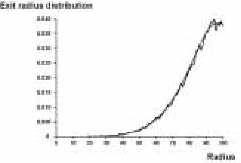
Fig. 3: Mean exit points distribution. The theoretical distribution (dashed line) is tested against the empirical one (solid line) obtained by running a simulation of 20 000 Brownian particles, starting on the wedge bisectrix ($\theta_{0}=\frac{\Theta}{2}$ at $r_{0}=R=100$ for $\Theta=\frac{\pi}{6}$). Because the starting point is located on the bisectrix, $\epsilon^{0}\left(x\right)=\epsilon^{\Theta}\left(x\right),$ and thus the analytical curve is given by $\epsilon\left(r\right)=\epsilon^{0}\left(r\right)+\epsilon^{\Theta}\left(r\right)=\frac{2}{\Theta r}\left(\frac{\left(rr_{0}\right)^{\left(\nu\right)}}{r^{2\nu}+r_{0}^{2\nu}}+\frac{\left(rr_{0}R^{2}\right)^{\left(\nu\right)}}{\left(rr_{0}\right)^{2\nu}+R^{4\nu}}\right)$. In that case, the maximum of the function $\epsilon\left(r\right)$ is achieved at $r=r_{0}e^{\frac{1}{2\nu}ln\left(\frac{\nu-1}{\nu+1}\right)}.$

3.4 The Mean Exit Radius (MER)

To determine the mean exit distribution radius $\overline{\epsilon}\left(r|r_{0}\right)$ for a viral particle starting initially at position $r_{0},\theta_{0}$ where $\theta_{0}$ is uniformly distributed between $0$ and $\Theta$, we consider $\epsilon\left(r|r_{0},\theta_{0}\right)=\epsilon^{0}\left(r|r_{0},\theta_{0}\right)+\epsilon^{\Theta}\left(r|r_{0},\theta_{0}\right)$ and estimate the integral

$$\overline{\epsilon}\left(r|r_{0}\right)=\frac{1}{\Theta}\int_{\Theta_{0}=0}^{\Theta}\epsilon\left(r|r_{0},\theta_{0}\right)d\theta_{0}.$$ (35)

Integrating expressions ((33) and (34)) we get :

$$\overline{\epsilon}\left(r|r_{0}\right)=\frac{2}{\Theta\pi r}\left(ln\left(\frac{r^{\nu}+r_{0}^{\nu}}{|r^{\nu}-r_{0}^{\nu}|}\right)+ln\left(\frac{R^{2\nu}+\left(rr_{0}\right)^{\nu}}{R^{2\nu}-\left(rr_{0}\right)^{\nu}}\right)\right).$$

We define the mean exit point as $r_{m}\left(r_{0}\right)=\mathbf{E}\left(r|r_{0}\right)$ conditioned on the initial radius $r_{0}$. Thus,

$$r_{m}\left(r_{0}\right)=\mathbf{E}\left(r|r_{0}\right)=\int_{0}^{R}r\overline{\epsilon}\left(r|r_{0}\right)dr.$$ (36)

Using the expansion $ln\left(1+x\right)=\sum_{n\geq 1}\left(-1\right)^{n+1}\frac{x^{n}}{n}$ for $x<1$, we obtain by a direct integration that

$$r_{m}\left(r_{0}\right)=\frac{8}{\pi^{2}}\left(r_{0}\left(\sum_{n=0}^{\infty}\frac{1}{\left(2n+1\right)^{2}}\left(\frac{1}{1-\frac{1}{\left(2n+1\right)^{2}\left(\frac{\pi}{\Theta}\right)^{2}}}\right)\right)-R\left(\sum_{n=0}^{\infty}\frac{\left(\frac{r_{0}}{R}\right)^{\left(2n+1\right)\frac{\pi}{\Theta}}\frac{\pi}{\Theta}}{\left(2n+1\right)\left(\left(\left(2n+1\right)\frac{\pi}{\Theta}\right)^{2}-1\right)}\right)\right),$$ (37)

using the expansion in the first part,

$$\frac{1}{1-\frac{1}{\left(2n+1\right)^{2}\left(\frac{\pi}{\Theta}\right)^{2}}}=\sum_{p=0}^{\infty}\left(\frac{\Theta}{\left(2n+1\right)\pi}\right)^{2p}$$ (38)

and the approximation $\Theta<<1$, we obtain using the value of the Riemann $\zeta-$function, $\zeta\left(2\right)=\frac{\pi^{2}}{6}$ and $\zeta\left(4\right)=\frac{\pi^{4}}{90}$, $r_{0}\leq R$, that

$${r_{m}\left(r_{0}\right)\approx r_{0}\left(1+\frac{\Theta^{2}}{12}\right)-\frac{8R}{\pi^{2}}\left(\frac{r_{0}}{R}\right)^{\pi/\Theta}\frac{\pi/\Theta}{\left(\pi/\Theta\right)^{2}-1}}.$$ (39)

For $\Theta$ small, the second term in the right-hand side of (39) is exponentially small.

4 Approximation of a virus motion by an effective Markovian stochastic equation

We replace the successive steps of viral dynamics with an effective stochastic equation containing a constant steady state drift.

4.1 Methodology

Virus motion described in paragraph (2.2) consists of a succession of drift and diffusing periods. We start with the stochastic equation

$$\mathbf{\dot{X}}=-B\frac{\mathbf{r}}{|\mathbf{r}|}+\sqrt{2D}\mathbf{\dot{w}},$$ (40)

where $r$ is the radial component of $\mathbf{X}$ , $B$ is the amplitude of the drift. The MFPT of the process (40) to the nucleus located $r=\delta$, when the initial position is located on the cell surface $r=R$ is solution of

$$D\left(\frac{d^{2}t}{dr^{2}}+\frac{1}{r}\frac{dt}{dr}\right)\left(r,\theta\right)-B\frac{dt}{dr}\left(r,\theta\right) = -1\hbox{ for }\left(r,\theta\right)\in\Omega$$

$$t\left(r,\theta\right) = 0\hbox{ for }r=\delta$$

$$\frac{dt}{dr}\left(r,\theta\right) = 0\hbox{ for }r=R.$$

A similar equation can be written in the domain $\tilde{\Omega}$ with reflective boundary conditions of the wedge. Both processes in the full domain or in $\tilde{\Omega}$ lead to the same MFPT. The solution $t(B,r)$ is given by

$$t\left(B,r\right)=C-\int_{r}^{R}\left(\int_{v}^{R}\frac{ue^{-\alpha\left(u-v\right)}}{Dv}du\right)dv,$$ (41)

where $\alpha=\frac{B}{D}$ and

$$t\left(B,R\right)=C=\int_{\delta}^{R}\left(\int_{v}^{R}\frac{ue^{-\alpha\left(u-v\right)}}{Dv}du\right)dv.$$ (42)

For a fixed radius R, the derivative of the function $t\left(B,R\right)$ with respect to B is strictly negative, which shows that $B\rightarrow t\left(B,R\right)$ is strictly decreasing. To determine the value of the amplitude $B$, we equal the mean time $t\left(B,R\right)$ with the MFPT to reach the nucleus within the iterative procedure as described in paragraph (2.2): at time zero, the virus starts at a position $r=R=R_{0}$ and reaches the edge boundary in a mean time $\bar{u}\left(R_{0}\right)$ and at a mean position $r_{m}\left(R_{0}\right)$. The viral particle is then transported toward the nucleus over a distance $d_{m}$ during a time $t_{m}$. Either the particle reaches the nucleus before time $t_{m}$ and then the algorithm is terminated or in a second step, it starts at a position $R_{1}=r_{m}\left(R_{0}\right)-d_{m}$. The process iterates until the particle reaches the nucleus. We consider the mean number of fundamental steps (diffusion step and directed motion along a MT step) the virus needs to reach the nucleus is equal to $n\geq 0$. The mean time to reach the nucleus computed by equation (41) has thus to be equal to the mean time $\tau=\sum_{k=0}^{n-1}\bar{u}(R_{k})+nt_{m}+<t_{r}>$ of the iterative trajectory. In a first approximation, we neglect the mean residual time $<t_{r}>$ and we thus get the equality:

$$t\left(B,R\right)=\tau=\sum_{k=0}^{n-1}\bar{u}\left(R_{k}\right)+nt_{m}$$ (43)

$$R_{k+1}=r_{m}\left(R_{k}\right)-d_{m}$$ (44)

$$R_{0}=R\hbox{ .}$$ (45)

For a fix radius R, equation (43) has a unique solution B, which can be found in practice by any standard numerical method.

Remark

The MFPT of a particle where the trajectory consists of alternating drift (traveling along microtubules) and diffusion periods can either be higher or lower than the MFPT of a pure Brownian particle. Indeed when $B<0$, the drift effect is less efficient than pure diffusion. For example, for $\Theta=\frac{\pi}{6}$, $R=100\mu m$, $\delta=\frac{R}{4}=25\mu m$, a large diffusion constant $D=10\mu m^{2}s^{-1}$ with the dynamical parameters $t_{m}=1s$ and $d_{m}=1\mu m$, leads to a negative mean drift

$$B\approx-0.14\mu ms^{-1}.$$ (46)

On the other hand, for a small diffusion constant $D=1\mu m^{2}s^{-1}$, an efficient microtubules transport obtained for $t_{m}=1s$ and $d_{m}=5\mu m$ leads to a mean positive drift

$$B\approx 0.13\mu ms^{-1}.$$ (47)

4.2 Explicit expression of the drift in the limit of $\Theta<<1$

When the number of microtubules is large enough, the condition $\Theta<<1$ is satisfied. Moreover, because a virus entering a cell surface has a deterministic motion, we can assume that the initial position satisfies $R_{0}<R$ so that we can neglect any boundary effects and use the open wedge approximation which consists of using formula (39) without the boundary layer term. Actually, this approximation is not that restrictive because after the first iteration process (movement along the microtubule followed by the particle release), the boundary layer term is negligible compared to the other term.

To obtain an explicit expression for the amplitude B, we consider the successive approximations

$$r_{m}\left(R_{0}\right)\approx R_{0}\left(1+\frac{\Theta^{2}}{12}\right),$$ (48)

and

$$R_{0} = R_{0};$$

$$R_{1} \simeq R_{0}\left(1+\frac{\Theta^{2}}{12}\right)-d_{m};$$

$$R_{2} \simeq R_{0}\left(1+\frac{\Theta^{2}}{12}\right)^{2}-d_{m}\left(1+\left(1+\frac{\Theta^{2}}{12}\right)\right);$$

$$\vdots$$

$$R_{i} \simeq R_{0}\left(1+\frac{\Theta^{2}}{12}\right)^{i}-d_{m}\left(\sum_{k=0}^{i-1}\left(1+\frac{\Theta^{2}}{12}\right)^{k}\right);$$

that is

$$R_{i}\simeq\left(R_{0}-\frac{12d_{m}}{\Theta^{2}}\right)\left(1+\frac{\Theta^{2}}{12}\right)^{i}+\frac{12d_{m}}{\Theta^{2}}.$$ (49)

Thus the particle reaches the nucleus after $n$ iteration steps which approximatively satisfies $R_{n}=\delta$,

$$n\simeq\displaystyle{\frac{ln\left(\frac{1-\frac{\delta\Theta^{2}}{12d_{m}}}{1-\frac{R_{0}\Theta^{2}}{12d_{m}}}\right)}{ln\left(1+\frac{\Theta^{2}}{12}\right)}}\approx\frac{R_{0}-\delta}{d_{m}}+o\left(1\right).$$ (50)

If $T_{n}$ denotes the mean time a viral particle takes to reach the nucleus, then using formula (18), we obtain

$$T_{n}\simeq n.t_{m}+\frac{\left(\frac{tan\left(\Theta\right)}{\Theta}-1\right)}{4D}\sum_{i=0}^{n-1}R_{i}^{2}\hbox{ ,}$$ (51)

that is

$$t \simeq n.t_{m}+\frac{\left(\frac{tan\left(\Theta\right)}{\Theta}-1\right)}{4D}$$

$$\sum_{i=0}^{n-1}\left(\left(\frac{12d_{m}}{\Theta^{2}}\right)^{2}+2\left(\frac{12d_{m}}{\Theta^{2}}\right)\left(R_{0}-\frac{12d_{m}}{\Theta^{2}}\right)\left(1+\frac{\Theta^{2}}{12}\right)^{i}+\left(R_{0}-\frac{12d_{m}}{\Theta^{2}}\right)^{2}\left(1+\frac{\Theta^{2}}{12}\right)^{2i}\right),$$

$$T_{n} \simeq nt_{m}+\frac{\left(\frac{tan\left(\Theta\right)}{\Theta}-1\right)}{4D}$$

$$\left(n\left(\frac{12d_{m}}{\Theta^{2}}\right)^{2}-\left(\frac{24d_{m}}{\Theta^{2}}\right)\left(R_{0}-\frac{12d_{m}}{\Theta^{2}}\right)\frac{1-\left(1+\frac{\Theta^{2}}{12}\right)^{n}}{\frac{\Theta^{2}}{12}}+\left(R_{0}-\frac{12d_{m}}{\Theta^{2}}\right)^{2}\frac{1-\left(1+\frac{\Theta^{2}}{12}\right)^{2n}}{1-\left(1+\frac{\Theta^{2}}{12}\right)^{2}}\right).$$

For $\Theta<<1$, a Taylor expansion gives that

$$T_{n} \simeq \left(\frac{R_{0}-\delta}{d_{m}}\right)t_{m}+\frac{t_{m}\left(R_{0}-\delta\right)}{24d_{m}}\left(1+\frac{R_{0}+\delta}{d_{m}}\right)\Theta^{2}$$

$$+ \frac{\left(R_{0}-\delta\right)}{72D}\left(d_{m}+3\left(R_{0}+\delta\right)+\frac{2\left(R_{0}^{2}+R_{0}\delta+\delta^{2}\right)}{d_{m}}\right)\Theta^{4}+o\left(\Theta^{4}\right).$$

In small diffusion limit $D<<1,\Theta<<1$, the velocity is $B\simeq\frac{R_{0}-\delta}{T_{n}}$ and consequently we obtain for $R_{0}\approx R$, a second order approximation

$$B\approx\frac{\frac{d_{m}}{t_{m}}}{1+\left(1+\frac{R+\delta}{d_{m}}\right)\frac{\Theta^{2}}{24}+O\left(\Theta^{4}\right)},$$ (52)

where $d_{m},{t_{m}}$ are the mean distance and the mean time a virus stays on the microtubule, R (resp. $\delta$) is the radius of the cell (resp. nucleus) and $\Theta=\frac{2\pi}{N}$, where N is the total number of microtubules.

4.3 Justification of the MFPT-criteria.

To justify the use of the MFPT-criteria to estimate the steady state drift, we run numerical simulations of 1,000 viruses inside a two dimensional domain $\Omega$ ($\delta<r<R$) with intermittent dynamics, alternating between epochs of free diffusion and directed motion along microtubules and compare the steady state distribution with the one obtained by solving the Fokker-Planck equation for viruses whose trajectories are described by the effective stochastic equation (5) with our computed constant drift

$$\mathbf{b}\left(\mathbf{X}\right)=-\frac{\frac{d_{m}}{t_{m}}}{1+\left(1+\frac{R+\delta}{d_{m}}\right)\frac{\Theta^{2}}{24}}\frac{\mathbf{r}}{|\mathbf{r}|}=-B\frac{\mathbf{r}}{|\mathbf{r}|}.$$ (53)

We imposed reflecting boundary conditions at the nuclear and the external membrane. The theoretical normalized steady state distribution $\rho$ satisfies

$$D\Delta\rho-\nabla.[\mathbf{b}\rho] = 0\hbox{ in }\Omega$$

$$\frac{d\rho}{dr}\left(R\right)=\frac{d\rho}{dr}\left(\delta\right) = 0.$$

and the solution $\rho$ is given by

$$\rho(r)=\frac{e^{-\frac{Br}{D}}}{\int_{\delta}^{R}e^{-\frac{Br}{D}}2\pi rdr}=\frac{e^{-\frac{Br}{D}}}{2\pi\frac{D}{B}\left(\delta e^{-\frac{B\delta}{D}}-Re^{-\frac{BR}{D}}+\frac{D}{B}\left(e^{-\frac{B\delta}{D}}-e^{-\frac{BR}{D}}\right)\right)}.$$ (54)

The result of both distributions is presented in figure 4 where we can observe that both curves match very nicely. This result shows that the criteria we have used is at least enough to recover the distribution. For the simulations, we consider the directed run of the virus along a MT (loaded by dynein) lasts $t_{m}=1s$ and covers a mean distance $d_{m}=0.7\mu m$ [13]. The diffusion constant is $D=1.3\mu m^{2}s^{-1}$ as observed for the Adeno Associated Virus [14].

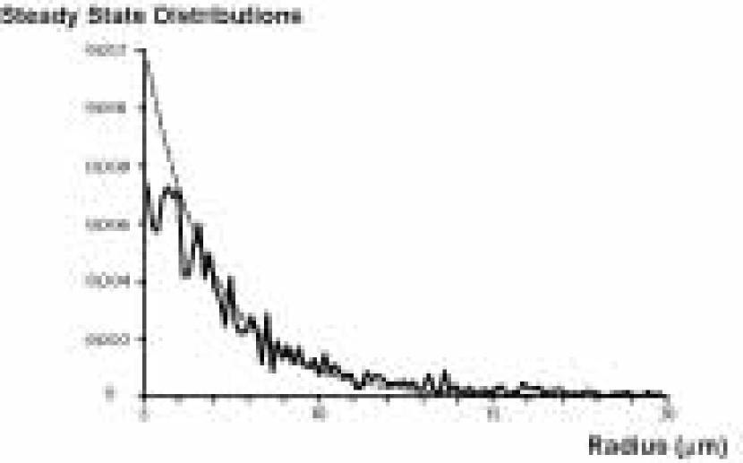
Fig. 4: Steady State distributions. We show the empirical steady state distribution for $1,000$ viral trajectories with an intermittent dynamic (solid line). The theoretical distribution of viruses whose trajectories are described by the stochastic equation (5) is given in dashed line. Geometrical parameters are : $R=20\mu m$, $\delta=5\mu m$ and $\Theta=\frac{\pi}{24}$.

The two curves in figure 4 fit very nicely except at the neighborhood of the nuclear membrane, where the simulation of the empirical distribution is plagued with a possible boundary layer. Another source of discrepancy comes from the difference of behavior of viruses far and close to the nucleus: viruses far from the nucleus do not bind as often as those located in its neighborhood. Consequently, a constant effective drift cannot account for the radial geometry near the nucleus. A theory for radius dependent effective drift has been derived in [15].

5 Conclusion

In the limit of a cell containing an excess of microtubules, we have presented here a model to describe the motion of biological particles such as viruses, vesicles and many others moving inside the cell cytoplasm by a complex combination of Brownian motion and deterministic drift. Our procedure consists mainly in approximating an alternative switching mode between diffusion and deterministic drift epochs by a steady state stochastic equation. This procedure consists of estimating the amplitude of the effective drift and is based on the criteria that the MFPTs to the nucleus, computed in both cases are equaled. In that case, this amplitude account for the directed transport along microtubules, the cell geometry and the binding constants. The model has however several limitations. First, we do not take into account directly the backward movement of the virus along the microtubules [16, 17], which can affect the mean time and the amplitude of the drift. Second, the present computations are given for two dimensional cell geometry only. It can still be applied to many in vitro culture cells, however it is not clear how to generalize our approach to a three dimensional cell geometry. For example, to study the trafficking inside cylindrical axons or dendrites of neuronal cells, a different approach should include this geometrical features. However despite these real difficulties, the present model may be used to analyze plasmid transport in an host cell, at the molecular level, which is one of the fundamental limitation of gene delivery [18, 19, 20, 21].

Appendix

In this appendix, we provide an explicit computation of integral (30) using the method of the residues. This method was previously used in a similar context in ([12] p 386). We denote by $\left(p_{j}^{k}\right)_{j\geq 0}$ the poles of the function

$$\Phi:s\rightarrow\frac{I_{k}\left(x\left(s\right)\wedge x_{0}\left(s\right)\right)\left(I^{{}^{\prime}}_{k}\left(x_{+}\left(s\right)\right)K_{k}-K^{{}^{\prime}}_{k}\left(x_{+}\left(s\right)\right)I_{k}\right)\left(x\left(s\right)\vee x_{0}\left(s\right)\right)}{sI^{{}^{\prime}}_{k}\left(x_{+}\left(s\right)\right)}e^{st}.$$

where ($x\left(s\right)=r\sqrt{\frac{s}{D}}$ , $x_{0}\left(s\right)=r_{0}\sqrt{\frac{s}{D}}$ and $x_{+}\left(s\right)=R\sqrt{\frac{s}{D}})$. The associated residues are $\left(r_{j}^{k}\right)_{j\geq 0}$. We now compute the residues explicitly.

To identify the poles, we recall the relation between the $k$-order Bessel’s function $J_{k}$ (that is true for $z$ such that $-\pi<arg\left(z\right)<\frac{\pi}{2}$) and the modified Bessel functions $I_{k}$ (p 375 [11]):

$$I_{k}\left(z\right)=e^{-\frac{1}{2}k\pi i}J_{k}\left(ze^{\frac{1}{2}\pi i}\right).$$ (55)

All roots $\alpha_{j,k}$ of the equations

$$J^{{}^{\prime}}_{k}\left(R\alpha\right)=0,$$

are real, simple and strictly positive (p 370 [11]) because $k$ is real and

$$k\leq\alpha_{1,k}<\alpha_{2,k}\ldots$$

Thus,

$$I^{{}^{\prime}}_{k}\left(-iR\alpha_{j,k}\right)=0.$$

Finally the poles of $\Phi$ are simple given by $p_{0}^{k}=0$ and $\forall j\geq 1$, $p_{j}^{k}=-D\alpha_{j,k}^{2}$. Consequently the associated residues are given for each $k$ for all $j\geq 0$ by

$$r_{j}^{k}=\lim_{s\rightarrow p_{j}^{k}}\left(s-p_{j}^{k}\right)\Phi(s).$$ (56)

Then using the residues, integral (30) is given by

$$I\left(r,\theta,t\right)=\frac{1}{\Theta\pi Di}\sum_{k}sin\left(k\theta\right)sin\left(k\theta_{0}\right)\left(2\pi i\right)\sum_{j\geq 0}r_{j}^{k}=\frac{2}{\Theta D}\sum_{k}sin\left(k\theta\right)sin\left(k\theta_{0}\right)\sum_{j\geq 0}r_{j}^{k}.$$

We now compute the residues $r_{j}^{k}.$ The residue $r_{0}^{k}$ is associated with the pole $p_{0}^{k}=0$ and given by

$$r_{0}^{k}=\lim_{s\rightarrow 0}s\Phi(s)$$

Using the following identities on the modified Bessel functions (p 489 [12])

$$I^{{}^{\prime}}_{k}\left(z\right)=I_{k+1}\left(z\right)+\frac{k}{z}I_{k}\left(z\right)\hbox{ and }K^{{}^{\prime}}_{k}\left(z\right)=-K_{k-1}\left(z\right)-\frac{k}{z}K_{k}\left(z\right),$$

substituting the derivatives $I^{{}^{\prime}}_{k}$ and $K^{{}^{\prime}}_{k}$ in the expression of $\Phi$, we get

$$r_{0}^{k} = \lim_{s\rightarrow 0}\frac{I_{k}\left(x\left(s\right)\wedge x_{0}\left(s\right)\right)}{\left(I_{k+1}+\frac{k}{x_{+}\left(s\right)}I_{k}\right)\left(x_{+}\left(s\right)\right)}$$

$$\left(\left(\left(I_{k+1}+\frac{k}{x_{+}\left(s\right)}I_{k}\right)\left(x_{+}\left(s\right)\right)K_{k}\right)+\left(\left(K_{k-1}+\frac{k}{x_{+}\left(s\right)}K_{k}\right)\left(x_{+}\left(s\right)\right)I_{k}\right)\right)\left(x\left(s\right)\vee x_{0}\left(s\right)\right),$$

Taking into account the dominant terms only, we get

$$r_{0}^{k}=\lim_{s\rightarrow 0}\frac{I_{k}\left(x\left(s\right)\wedge x_{0}\left(s\right)\right)\left(I_{k}\left(x_{+}\left(s\right)\right)K_{k}+K_{k}\left(x_{+}\left(s\right)\right)I_{k}\right)\left(x\left(s\right)\vee x_{0}\left(s\right)\right)}{I_{k}\left(x_{+}\left(s\right)\right)}.$$

To further compute this limit, we use the Taylor expansions of $I_{k}$ and $K_{k}$ (p 375 [11]) expressed in terms of the $\Gamma$ function:

$$I_{k}\left(z\right) \approx \frac{\left(\frac{1}{2}z\right)^{k}}{\Gamma\left(k+1\right)}\hbox{ and }K_{k}\left(z\right)\approx\frac{1}{2}\Gamma\left(k\right)\left(\frac{1}{2}z\right)^{-k}.$$

For $r<r_{0}$, we get

$$r_{0}^{k}=\lim_{s\rightarrow 0}\frac{\frac{\left(\frac{1}{2}\left(x\left(s\right)\right)\right)^{k}}{\Gamma\left(k+1\right)}\left(\frac{\left(\frac{1}{2}\left(x_{+}\left(s\right)\right)\right)^{k}}{\Gamma\left(k+1\right)}\frac{1}{2}\Gamma\left(k\right)\left(\frac{1}{2}\left(x_{0}\left(s\right)\right)\right)^{-k}+\frac{1}{2}\Gamma\left(k\right)\left(\frac{1}{2}\left(x_{+}\left(s\right)\right)\right)^{-k}\frac{\left(\frac{1}{2}\left(x_{0}\left(s\right)\right)\right)^{k}}{\Gamma\left(k+1\right)}\right)}{\frac{\left(\frac{1}{2}\left(x_{+}\left(s\right)\right)\right)^{k}}{\Gamma\left(k+1\right)}}.$$

Finally, using the relation $\Gamma\left(k+1\right)=k\Gamma\left(k\right)$, and the expressions of $x(s)$, $x_{0}(s)$ and $x_{+}(s)$ we get

$$r_{0}^{k}=\frac{r^{k}\left(r_{0}^{2k}+R^{2k}\right)}{2kR^{2k}r_{0}^{k}}.$$

The computation of the other residues $\left(r_{j}^{k}\right)_{j\geq 1}$, is slightly different

$$r_{j}^{k}=\lim_{s\rightarrow p_{j}^{k}}\left(s-p^{k}_{j}\right)\Phi(s),$$

where $p_{j}^{k}=-D\alpha^{2}_{j,k}$. Using the Wronskian relation (p 489 [12]) :

$$I_{k}\left(z\right)K^{\prime}_{k}\left(z\right)-K_{k}\left(z\right)I^{\prime}_{k}\left(z\right)=-\frac{1}{z},$$

we now substitute

$$K_{k}^{{}^{\prime}}\left(z\right)=\frac{-\frac{1}{z}+K_{k}\left(z\right)I^{{}^{\prime}}_{k}\left(z\right)}{I_{k}\left(z\right)}.$$

in the expression of $\Phi$, we get

$$r_{j}^{k}=\lim_{s\rightarrow p_{j}^{k}}\frac{\left(s-p_{j}^{k}\right)e^{st}}{s}\frac{I_{k}\left(x\left(s\right)\right)\left(I^{{}^{\prime}}_{k}\left(x_{+}\left(s\right)\right)K_{k}-\left(\frac{-\frac{1}{x_{+}\left(s\right)}+K_{k}I^{{}^{\prime}}_{k}}{I_{k}}\right)\left(x_{+}\left(s\right)\right)I_{k}\right)\left(x_{0}\left(s\right)\right)}{I^{{}^{\prime}}_{k}\left(x_{+}\left(s\right)\right)}.$$

Because

$$\lim_{s\rightarrow p_{j}^{k}}I^{{}^{\prime}}_{k}\left(x_{+}\left(s\right)\right)=I^{{}^{\prime}}_{k}\left(x_{+}\left(p_{j}^{k}\right)\right)=0,$$

we obtain the expression for the residues:

$$r_{j}^{k}=\frac{e^{p_{j}^{k}t}}{p_{j}^{k}}\frac{I_{k}\left(x\left(p_{j}^{k}\right)\right)I_{k}\left(x_{0}\left(p_{j}^{k}\right)\right)}{I_{k}\left(x_{+}\left(p_{j}^{k}\right)\right)x_{+}\left(p_{j}^{k}\right)}\lim_{s\rightarrow p_{j}^{k}}\frac{\left(s-p^{k}_{j}\right)}{I^{{}^{\prime}}_{k}\left(x_{+}\left(s\right)\right)}.$$

Finally, since

$$\lim_{s\rightarrow p_{j}^{k}}\frac{\left(s-p^{k}_{j}\right)}{I^{{}^{\prime}}_{k}\left(x_{+}\left(s\right)\right)}=\frac{2\sqrt{Dp_{j}^{k}}}{R}\lim_{s\rightarrow p_{j}^{k}}\frac{x_{+}\left(s\right)-x_{+}\left(p_{j}^{k}\right)}{I^{{}^{\prime}}_{k}\left(x_{+}\left(s\right)\right)-I^{{}^{\prime}}_{k}\left(x_{+}\left(p_{j}^{k}\right)\right)}=\frac{2\sqrt{Dp_{j}^{k}}}{RI^{{}^{\prime\prime}}_{k}\left(x_{+}\left(p_{j}^{k}\right)\right)},$$

we obtain

$$r_{j}^{k}=\frac{e^{p_{j}^{k}t}}{p_{j}^{k}}\frac{I_{k}\left(x\left(p_{j}^{k}\right)\right)I_{k}\left(x_{0}\left(p_{j}^{k}\right)\right)}{I_{k}\left(x_{+}\left(p_{j}^{k}\right)\right)x_{+}\left(p_{j}^{k}\right)}\frac{2\sqrt{Dp_{j}^{k}}}{RI^{{}^{\prime\prime}}_{k}\left(x_{+}\left(p_{j}^{k}\right)\right)}.$$

To simplify this expression, we use that $I_{k}$ satisfies the differential equation (p 374 [11]):

$$I^{{}^{\prime\prime}}_{k}\left(z\right)+\frac{1}{z}I^{{}^{\prime}}_{k}\left(z\right)-\left(1+\frac{k^{2}}{z^{2}}\right)I_{k}\left(z\right)=0,$$

thus for $z=x_{+}\left(p_{j}^{k}\right)$ :

$$I^{{}^{\prime\prime}}_{k}\left(x_{+}\left(p_{j}^{k}\right)\right)=\frac{p_{j}^{k}R^{2}+Dk^{2}}{p_{j}^{k}R^{2}}I_{k}\left(x_{+}\left(p_{j}^{k}\right)\right),$$

we get

$$r_{j}^{k}=\frac{2De^{p_{j}^{k}t}}{R^{2}p_{j}^{k}+Dk^{2}}\frac{I_{k}\left(x\left(p_{j}^{k}\right)\right)I_{k}\left(x_{0}\left(p_{j}^{k}\right)\right)}{I^{2}_{k}\left(x_{+}\left(p_{j}^{k}\right)\right)},$$

and finally, using (55), we get

$$r_{j}^{k}=\frac{2e^{-D\alpha^{2}_{j,k}t}}{-R^{2}\alpha^{2}_{j,k}+k^{2}}\frac{J_{k}\left(r\alpha_{j,k}\right)J_{k}\left(r_{0}\alpha_{j,k}\right)}{J^{2}_{k}\left(R\alpha_{j,k}\right)}.$$

Integral (30) is given by

$$I(r,\theta,t)=\frac{2}{\Theta D}\sum_{k}sin\left(k\theta\right)sin\left(k\theta_{0}\right)\sum_{j\geq 0}r_{j}^{k}=\frac{2}{\Theta D}\left(S_{1}(r,\theta,t)+S_{2}(r,\theta,t)\right).$$ (57)

where

$$\displaystyle{S_{1}(r,\theta,t)} = \displaystyle{\sum_{k}sin\left(k\theta\right)sin\left(k\theta_{0}\right)\frac{r^{k}\left(r_{0}^{2k}+R^{2k}\right)}{2kR^{2k}r_{0}^{k}},}$$

$$\displaystyle{S_{2}(r,\theta,t)} = \displaystyle{-2\sum_{k}sin\left(k\theta\right)sin\left(k\theta_{0}\right)\sum_{j=1}^{\infty}e^{-D\alpha_{j,k}^{2}t}\frac{J_{k}\left(r\alpha_{j,k}\right)J_{k}\left(r_{0}\alpha_{j,k}\right)}{\left(R^{2}\alpha_{j,k}^{2}-k^{2}\right)J^{2}_{k}\left(R\alpha_{j,k}\right)}},$$

References

- [1] Wiethoff C. M. Wiethoff and C. R. Middaugh, Barriers to Non-Viral Gene Delivery, Journal of Pharmaceutical Sciences, 92 (2003), pp. 203–217.
- [2] D. Dauty and A. S. Verkman, Actin Cytoskeleton as the Principal Determinant of Size-Dependent DNA Mobility in Cytoplasm: a New Barrier for Non-Viral Gene Delivery, Journal of Biological Chemistry, 280 (2005), pp. 7823–7828.
- [3] A. T. Dinh, T. Theofanous and S. Mitragotri, A Model for Intracellular Trafficking of Adenoviral Vectors, Biophysical Journal, 89 (2005), pp. 1574–1588.
- [4] B. Alberts, A. Johnson, J. Lewis, M. Raff , K. Roberts and P. Walter, Molecular Biology of the Cell, 4th Edition, Garland, New-York 2002.
- [5] D. Holcman, Modeling Trafficking of a Virus and a DNA Particle in the Cell Cytoplasm, Journal of Statistical Physics, 127 (2007), pp. 471–494.
- [6] Z. Schuss, Theory and Applications of Stochastic Differential Equations, John Wiley & Sons Inc, New-York 1981.
- [7] N. Hirokawa, Kinesin and Dynein Superfamily Proteins and the Mechanism of Organelle Transport, Science, 279 (1998), pp. 519–526.
- [8] R. Mallick, Cytoplasmic Dynein Functions as a Gear in Response to Load, Nature, 427 (2004), pp. 649–652.
- [9] S. Redner, A Guide to First Passage Processes, Cambridge University Press, Cambridge, Massachussets, 2001.
- [10] P. Henrici, Applied and Computational Complex Analysis. Vol. 3., John Wiley & Sons Inc, New-York 1977.
- [11] M. Abramowitz, and I. A. Stegun, Handbook of Mathematical Functions, Dover, New York 1972.
- [12] H. S. Carslaw, and J. C. Jaegger, Conduction of Heat in Solids, Oxford University Press, Oxford, U.K. 1959.
- [13] S. J. King and T. A Schroer, Dynactin Increases the Processivity of the Cytoplasmic Dynein Motor, Nat. Cell Biol., 2 (2000), pp. 20–24.
- [14] G. Seisenberger et al., Real-Time Single-Molecule Imaging of the Infection Pathway of an Adeno-Associated Virus, Science, 294 (2001), pp. 1929–1932.
- [15] T. Lagache et D. Holcman, Quantifying the Intermittent Transport in the Cell Cytoplasm (submitted).
- [16] D. Katinka, N.Claus-Henning, and B. Sodeik, Viral Stop-and-Go along Microtubules : Taking a Ride with Dynein and Kinesins, Trends in Microbiology, 13(7) (2005), pp. 320–327.
- [17] S. P. Gross, M. A Welte, S. M. Block, and E. F. Wieschaus, Dynein-mediated Cargo Transport in Vivo : a Switch Controls Travel Distance, The Journal of Cell Biology, 5 (2000), pp. 945–955.
- [18] G. R. Whittaker, Virus Nuclear Import, Advanced Drug Delivery Rewiews, 55 (2003), pp. 733–747.
- [19] D. A. Dean, R. C. Geiger, and R. Zhou, Intracellular Trafficking of Nucleic Acids, Expert Opinion Drug Delivery, 1 (2004), pp. 127–140.
- [20] E. M. Campbell, and T. J. Hope, Gene Therapy Progress and Prospects : Viral Trafficking During Infection, Gene Therapy, 12 (2005), pp. 1353–1359.
- [21] D. Luo, and W. M. Saltzman, Synthetic DNA Delivery Systems, Nature Biotechnology, 18 (1999), pp. 33–37.