Accurate calculation of the complex eigenvalues of the Schrödinger equation with an exponential potential

Abstract

We show that the Riccati–Padé method is suitable for the calculation of the complex eigenvalues of the Schrödinger equation with a repulsive exponential potential. The accuracy of the results is remarkable for realistic potential parameters.

1 Introduction

Recently, Rakityansky et al [1] developed a method for the calculation of bound states and resonances of quantum–mechanical problems. It is based on the approximation of the S–matrix by means of Padé approximants and the location of their poles. The authors mention that the methods for the calculation of bound states and resonances are usually developed separately in spite of the fact that those quantities share the same mathematical nature.

Some time ago we developed the Riccati–Padé method that applies to bound states and resonances of separable quantum–mechanical models [3, 2, 4, 5, 7, 8, 6, 9, 10, 11]. Although the RPM is less general than the approach proposed by Ratikyansky et al [1] it is nevertheless an interesting approach for comparison purposes and benchmark.

The RPM [3, 2, 4, 5, 7, 8, 6, 9, 10, 11] is based on a rational approximation to a modified logarithmic derivative of the wavefunction that satisfies a Riccati equation. From the coefficients of the Taylor expansion of this logarithmic derivative, which are functions of the energy, we construct Hankel determinants. Their roots give rise to sequences that converge towards the bound states and resonances of the quantum–mechanical model as the determinant dimension increases. In most cases the rate of convergence is so great that the RPM yields extremely accurate real and complex eigenvalues.

The rational approximation and the Hankel quantization condition appear to select square integrable functions and incoming or outgoing waves. Both, bound states and resonances emerge from the Hankel sequences because one does not introduce the boundary conditions at infinity explicitly.

Earlier results for exponential potentials suggest that the RPM may not yield virtual states and that the Hankel sequences converge to a wrong limit, although, suspiciously close to the right answer, in the case of some resonances[9]. The purpose of this paper is to investigate this feature of the RPM more closely.

In Section 2 we discuss a simple model that enables us to calculate the poles of the scattering amplitude from the roots of Bessel functions. In Section 3 we apply the RPM to this model and compare approximate and exact results. Finally, in Section 4 we summarize our results and draw conclusions.

2 Model

In this paper we test the performance of the RPM on the Schrödinger equation

$$\psi^{\prime\prime}(x)+\left(E-Ae^{-\alpha x}\right)\psi(x)=0$$ (1)

with the boundary condition $\psi(0)=0$. This model has proved useful in the past for the study of bound, resonance, and virtual states[12, 13, 14]. Besides, the exponential potential is a suitable representation of repulsive molecular interactions[13]. The change of variables $q=\alpha x$, $\Phi(q)=\psi(q/\alpha)$ leads to an eigenvalue equation with just one potential parameter:

$$\Phi^{\prime\prime}(q)+\left(\epsilon-\lambda e^{-q}\right)\Phi(q)=0$$ (2)

where $\epsilon=E/\alpha^{2}$ and $\lambda=A/\alpha^{2}$.

A further change of variables $z=2\sqrt{-\lambda}e^{-q/2}$, $Y(z)=\Phi(2\ln[2\sqrt{-\lambda}/z])$ transforms the eigenvalue equation (2) into the Bessel equation

$$z^{2}Y^{\prime\prime}(z)+zY^{\prime}(z)+\left(z^{2}-\nu^{2}\right)Y(z)=0$$ (3)

where $\nu^{2}=-4\epsilon$. The general solution that satisfies the boundary condition at $q=0$ is [12]

$$Y(z)=C\left[J_{-\nu}\left(2\sqrt{-\lambda}\right)J_{\nu}(z)-J_{\nu}\left(2\sqrt{-\lambda}\right)J_{-\nu}(z)\right]$$ (4)

If we assume that the RPM will provide the eigenvalues of those solutions that satisfy $\lim_{q\rightarrow\infty}\Phi(q)=0$, then it follows from the behaviour of the Bessel function at origin $J_{\nu}(z)\sim\left(z/2\right)^{\nu}/\Gamma(\nu+1)$ that they should be roots of

$$J_{\nu}\left(2\sqrt{-\lambda}\right)=0$$ (5)

with $\mathrm{Re}(\nu)>0$. The roots of this equation are poles of the scattering amplitude[13].

The modified logarithmic derivative of an eigenfunction of equation (2)

$$f(q)=\frac{1}{q}-\frac{\Phi^{\prime}(q)}{\Phi(q)}$$ (6)

satisfies the Riccati equation

$$f^{\prime}(q)+\frac{2f(q)}{q}-f(q)^{2}+\lambda e^{-q}-\epsilon=0$$ (7)

The Taylor series about the origin

$$f(q)=\sum_{j=0}^{\infty}f_{j}q^{j},\;f_{0}=0$$ (8)

converges in a neighbourhood of $q=0$ and the coefficients $f_{j}$ depend on $\epsilon$.

The main assumption of the RPM is that the roots of the Hankel determinants $H_{D}^{d}(\epsilon)=0$, with matrix elements $f_{j+j+d-1}$, $i,j=1,2,\ldots,D$, are suitable approximations to the eigenvalues of the Schrödinger equation (2)[3, 2, 4, 5, 7, 8, 6, 9, 10, 11]. Here, $D=2,3,\ldots$ is the determinant dimension and $d=0,1,\ldots$. More precisely, we expect that there exists a sequence of roots $\epsilon^{[D,d]}$ of the Hankel determinants that converges to a given eigenvalue of that Schrödinger equation as $D$ increases.

3 Results and discussion

Previous applications of the RPM showed that the rate of convergence of the Hankel sequences is remarkable for both real and complex eigenvalues[3, 2, 4, 5, 7, 8, 6, 9, 10, 11]. However, in the case of the exponential potential (1) the Hankel sequences were found to converge to a result slightly different from the one given by equation (5)[9]. For example, Table 1 shows Hankel sequences for $\lambda=0.5$ and $\lambda=2$ and the corresponding exact results obtained from the quantization condition (5). Both Hankel sequences exhibit great convergence rate but they do not converge towards the expected result. We also appreciate that the disagreement between the exact and RPM eigenvalues increases as $\lambda$ decreases. In addition to the great convergence rate, the Hankel determinants exhibit clustering of roots about the limits of the sequences as $D$ increases, which is an indication of satisfactory convergence and meaningful result. However, those limits do not completely agree with the exact results given by (5).

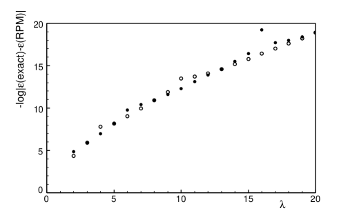
Figure 2: $\log|\mathrm{Re}\ \epsilon^{exact}-\mathrm{Re}\ \epsilon^{RPM}|$ (empty circles) and $\log|\mathrm{Im}\ \epsilon^{exact}-\mathrm{Im}\ \epsilon^{RPM}|$ (solid circles)

Fig. 1 shows values of $\epsilon(\lambda)$ calculated by means of the RPM and equation (5). As indicated above, the agreement between the RPM and exact results increases as $\lambda$ increases. For $\lambda\leq 0.4$ the RPM yields complex eigenvalues in spite of the fact that the exact ones are real (see, for example, Atabek et al[13] for a more detailed discussion of this behaviour). Moreover, it is well known that the roots $\nu$ of equation (5) tend to negative integers as $\lambda\rightarrow 0$[13, 14] but we clearly see that the RPM eigenvalues do not exhibit this behaviour. However, it is most interesting that both real and imaginary parts of the RPM eigenvalues give a reasonable picture of the behaviour of the exact ones for large and moderate values of $\lambda$ as shown in Fig. 1. In order to show the increasing agreement between the RPM and exact eigenvalue with $\lambda$ more clearly, Fig. 2 shows $\log|\epsilon^{exact}-\epsilon^{RPM}|$ as a function of $\lambda$.

The discrepancy between the RPM and exact eigenvalues just mentioned is interesting from a mathematical point of view, but it is not a serious drawback for physical purposes. It is well known that realistic potentials require much larger values of $\lambda$ than those in Fig. 1[13]. If, for example we choose $\lambda=100$ the rate of convergence of the Hankel sequence is much greater than the one in Table 1 and the limit agrees with the exact result to at least 20 digits (see Table 2). Atabek et al [13] estimated the potential parameter for the ${}^{2}\Sigma^{+}$ repulsive state of BeH to be $\Lambda\simeq 134$ that corresponds to $\lambda=4489$. In this case the rate of convergence of the Hankel sequence is even greater and we obtain the exact result to at least 20 digits with $D=15$ and $d=0$ as shown in Table 2. It is worth mentioning that for such large values of $\lambda$ we find it easier to obtain the complex energies by means of the RPM than from the roots of the Bessel function.

4 Conclusions

We have shown that the Hankel sequences converge to a wrong limit that is close to the resonances of the repulsive exponential potential. At present we do not know the reason for this discrepancy that decreases as the potential strength increases. However the RPM eigenvalue as function of the potential parameter follows the trend of the exact one. Besides, for realistic potential functions that fit the interaction between molecular fragments[13], the RPM provides remarkably accurate results and it is probably more accurate than other methods. Unfortunately we are not aware of results for such great values of the potential strength, probably because other methods do not provide the complex eigenvalues so efficiently as the RPM.

We should mention that the complex eigenvalues of the Schrödinger equation with the exponential potential (1) are not what physicist use to call resonances because the imaginary parts are too large. However, there has been some interest in their calculation with the purpose of reconstruction of the scattering amplitude from its poles[13, 14].

Table 1: Convergence of the Hankel sequences for two values of $\lambda$

$\lambda=0.5$
$D$	$\mathrm{Re}\ \epsilon$	$\mathrm{Im}\ \epsilon$
10	-0.70545054582805260895	0.26816598479688956569
11	-0.70545056661473611239	0.26816596401669675062
12	-0.70545056816101389381	0.26816596478162896896
13	-0.70545056810407142688	0.26816596486012868610
14	-0.70545056805626480670	0.26816596487152171555
15	-0.70545056805476309518	0.26816596487187249577
16	-0.70545056805499618233	0.26816596487156659341
17	-0.70545056805503003056	0.26816596487158015859
18	-0.70545056805502881287	0.26816596487157957123
19	-0.70545056805502843245	0.26816596487157970586
20	-0.70545056805502836237	0.26816596487157971713
$Exact$	-0.73985910415959609800	0.24527511363052010569
$\lambda=2$
$D$	$\mathrm{Re}\ \epsilon$	$\mathrm{Im}\ \epsilon$
10	-0.66695560251365514674	1.6211700286378446183
11	-0.66695559703717080232	1.6211700273918467827
12	-0.66695559708065060107	1.6211700264998970342
13	-0.66695559710083543597	1.6211700264601278937
14	-0.66695559710850847182	1.6211700264500121775
15	-0.66695559710929174524	1.6211700264509149572
16	-0.66695559710923347745	1.6211700264509352898
17	-0.66695559710922690796	1.6211700264509338670
18	-0.66695559710922683370	1.6211700264509344139
19	-0.66695559710922693659	1.6211700264509344652
20	-0.66695559710922696333	1.6211700264509344798
$Exact$	-0.66691308506826236505	1.6211836543647526877

Table 2: Convergence of the Hankel sequences for large values of $\lambda$

$\lambda=100$
$D$	$\mathrm{Re}\ \epsilon$	$\mathrm{Im}\ \epsilon$
5	71.535851840807002875	37.763655201763995538
6	71.535265703486635320	37.763686464878442119
7	71.535231112272632786	37.763673576025908553
8	71.535229874257576952	37.763674377953883589
9	71.535229860223483406	37.763674375421503193
10	71.535229855328822688	37.763674374272030169
11	71.535229855364554354	37.763674374318377973
12	71.535229855364593976	37.763674374316154213
13	71.535229855364798246	37.763674374316019149
14	71.535229855364801073	37.763674374316016150
15	71.535229855364801145	37.763674374316015925
16	71.535229855364801148	37.763674374316015917
17	71.535229855364801148	37.763674374316015916
$\lambda=4489$
$D$	$\mathrm{Re}\ \epsilon$	$\mathrm{Im}\ \epsilon$
5	4158.9571348913180566	530.18487292989576140
6	4158.9534557328433593	530.18603523832850612
7	4158.9533491082024576	530.18608879147133066
8	4158.9533468989068860	530.18609014361891762
9	4158.9533468479121394	530.18609015967783227
10	4158.9533468461423605	530.18609015977128983
11	4158.9533468460962321	530.18609015979497844
12	4158.9533468460956664	530.18609015979556450
13	4158.9533468460956584	530.18609015979556963
14	4158.9533468460956581	530.18609015979556941
15	4158.9533468460956580	530.18609015979556943
16	4158.9533468460956580	530.18609015979556943

Figure 1: Eigenvalues of the exponential potential: $\mathrm{Re}\ \epsilon^{RPM}$ (empty circles), $\mathrm{Im}\ \epsilon^{RPM}$ (solid circles), $\mathrm{Re}\ \epsilon^{exact}$ (dashed line), $\mathrm{Im}\ \epsilon^{exact}$ (solid line)

References

- [1] S. A. Rakityansky, S. A. Sofianos, and N. Elander, J. Phys. A 40 (2007) 14857-14869.
- [2] F. M. Fernández, Q. Ma, and R. H. Tipping, Phys. Rev. A 40 (1989) 6149-6153.
- [3] F. M. Fernández, Q. Ma, and R. H. Tipping, Phys. Rev. A 39 (1989) 1605-1609.
- [4] F. M. Fernández, Phys. Lett. A 166 (1992) 173-176.
- [5] F. M. Fernández and R. Guardiola, J. Phys. A 26 (1993) 7169-7180.
- [6] F. M. Fernández, Phys. Lett. A 203 (1995) 275-278.
- [7] F. M. Fernández, J. Phys. A 28 (1995) 4043-4051.
- [8] F. M. Fernández, J. Chem. Phys. 103 (1995) 6581-6585.
- [9] F. M. Fernández, J. Phys. A 29 (1996) 3167-3177.
- [10] F. M. Fernández, Phys. Rev. A 54 (1996) 1206-1209.
- [11] F. M. Fernández, Chem. Phys. Lett 281 (1997) 337-342.
- [12] S. T. Ma, Phys. Rev. 69 (1946) 668.
- [13] O. Atabek, R. Lefebvre, and M. Jacon, J. Phys. B 15 (1982) 2689-2701.
- [14] P. Midy, O. Atabek, and G. Oliver, J. Phys. B 26 (1993) 835-853.