Surprising relations between parametric level correlations and fidelity decay

Abstract

Relations between fidelity decay, cross form–factor (i.e., parametric level correlations), and level velocity correlations are found both by deriving a Ward identity in a two-matrix model, and by comparing exact results, using supersymmetry techniques, in the framework of random matrix theory. A power law decay near Heisenberg time, as a function of the relevant parameter, is shown to be at the root of revivals recently discovered for fidelity decay. For cross form–factors the revivals are illustrated by a numerical study of a multiply kicked Ising spin chain.

Fidelity decay presently attracts considerable attention Gorin et al. (2006). It measures the change of quantum dynamics of a state under a modification of the Hamiltonian. In quantum information, fidelity measures the deviation between a mathematical algorithm and its physical implementation. From a different point of view, important insight into the properties of the underlying systems is provided by the studies of correlations between spectra of random and/or chaotic Hamiltonians which differ by a parameter-dependent perturbation gen . Since statistical properties of fidelity decay in random/chaotic systems involve both spectra and eigenfunctions of the original and perturbed Hamiltonians, existence of any connections between fidelity and purely spectral correlations is not a priori obvious.

Random Matrix Theory (RMT) has been successful in describing quantum many-body systems and as model for the spectral properties of single particle systems whose classical analogue is chaotic Guhr et al. (1998). Within RMT fidelity was analyzed in linear response approximation Gorin et al. (2004) and both fidelity rud ; gor ; Stöckmann and Kohler (2006) and parametric correlations sim were calculated exactly using the supersymmetry method. An unexpected fidelity revival at Heisenberg time was encountered rud within RMT and confirmed in a dynamical coupled spin chain model Pineda et al. (2006).

Earlier, differential relations between parametric spectral correlations and parametric density correlations were established taniguchi (1, 2). By relating the latter to the fidelity amplitude via Fourier transform, we show in this letter that the existence of these relations opens a crucial insight into the properties of fidelity decay. By analyzing the characteristic features of the parametric correlations in the time domain, the cross–form factor, we discover a new, simple interpretation of the previously puzzling phenomenon of revival rud . These relations follow directly from the basic definitions and symmetries of the underlying matrix models, being essentially Ward identities. We show that they are valid under very general assumptions. No explicit (e.g., supersymmetric) calculation is required, however they rely on the universality of the parametric spectral correlations at the scale of mean level spacing. We thus explain the origin of various relations connecting spectral and wave-function correlations, and establish a unified framework for their analysis and generalizations. A relation between fidelity decay and level velocity correlation function is given. The latter is important from the experimental point of view, being used for independent access to system parameters. We confirm the general results comparing fidelity decay and cross–form factors in RMT. We illustrate our analytical results with a numerical study of a multiply kicked Ising spin chain.

We consider Hamiltonians modeled by $N\times N$ matrices

$$H^{\pm}(\lambda)\ =\ H\pm\lambda V/2\ ,$$ (1)

where $H$ and $V$ are independently drawn from ensembles of the same symmetry. In particular, $V$ is drawn from the GOE, the GUE or the GSE ensembles of RMT, labeled $\beta=1,2,4$. The ensemble average over both is indicated by angular brackets. It is convenient to fix the variances as $\langle H_{ij}H_{kl}\rangle$ $=D^{-1}\langle V_{ij}V_{kl}\rangle$ where $D$ is the mean level spacing of $H^{\pm}(0)$ in the energy region of interest. In the RMT case, $D=\pi^{2}/N$ in the center of the spectrum. The mean level spacing is then $\lambda$-independent up to corrections of order $1/N$. By construction, $H^{\pm}(\lambda)$ is in the same symmetry class as $H$ for any $\lambda$.

The parametric two–level correlation function is defined as

$$\widetilde{R}_{\beta}(E^{+},E^{-},\lambda)=\sum_{n,m}\langle\delta(E^{-}-\epsilon^{-}_{n}(\lambda))\delta(E^{+}-\epsilon^{+}_{m}(\lambda))\rangle\ .$$ (2)

It is mapped onto a dimensionless energy scale, where the mean level spacing is rescaled to unity. One has

$$\widetilde{X}_{\beta}(r,\lambda)=\lim_{N\to\infty}D^{2}\widetilde{R}_{\beta}(E^{+},E^{-},\lambda)\ ,$$ (3)

which solely depends on the difference $r=(E^{+}-E^{-})/D$. The cross form-factor is obtained as a Fourier transform

$$\widetilde{K}_{\beta}(t,\lambda)=\int_{-\infty}^{+\infty}\left(1-\widetilde{X}_{\beta}(r,\lambda)\right)e^{2\pi\imath tr}dr\,,\ t>0\ .$$ (4)

Time $t$ is measured in units of Heisenberg time $t_{H}=D^{-1}$. Fidelity decay is expressed via the echo operator Gorin et al. (2006)

$$M(t,\lambda)\ =\exp(\imath 2\pi tH^{-}(\lambda)/D)\,\exp(-\imath 2\pi tH^{+}(\lambda)/D)\ .$$ (5)

Its expectation value with a given state is the fidelity amplitude and its average

$$\quad f_{\beta}(t,\lambda)=\frac{1}{N}{\rm tr}\langle M(t,\lambda)\rangle$$ (6)

is a measure for the difference in the two time evolutions as a function of $\lambda$.

The functions in Eq. (3) were calculated exactly with the supersymmetry method sim for $\beta=1,2,4$. The Fourier transforms are (see also Mucciolo )

$$\widetilde{K}_{1}(t,\lambda)=\int_{\max(0,t-1)}^{t}du\int_{0}^{u}dv\frac{2t^{2}(t-u)(1-t+u)}{(v^{2}-t^{2})^{2}}\\ \times\frac{\exp\left(-2\pi^{2}\lambda^{2}\left[2ut+t-t^{2}+v^{2}\right]\right)}{\sqrt{(u^{2}-v^{2})(u^{2}+2u+1-v^{2})}},\\ \widetilde{K}_{2}(t,\lambda)=\frac{\exp\left(-2\pi^{2}\lambda^{2}t^{1+\theta(t-1)}\right)}{2\pi^{2}\lambda^{2}t}\sinh\left(2\pi^{2}\lambda^{2}t^{2-\theta(t-1)}\right)\ ,\\ \widetilde{K}_{4}(t,\lambda)=t^{2}\int_{-1}^{+1}du\int_{0}^{1-|u|}dv\frac{(u+t)^{2}-1}{(t^{2}-v^{2})^{2}}\\ \times\frac{v\theta(u-1+t)\exp\left(-\pi^{2}\lambda^{2}[t^{2}-v^{2}+2tu]\right)}{\sqrt{\left[(u-1)^{2}-v^{2}\right]\left[(u+1)^{2}-v^{2}\right]}},$$ (7)

with Heaviside’s $\theta$–function. For $\lambda=0$ the cross form-factors reduce to the standard form factors $K_{\beta}(t)$ Guhr et al. (1998), i.e. $\widetilde{K}_{\beta}(t,0)=K_{\beta}(t)$. In Fig. 1 we show $\widetilde{K}_{\beta}(t,\lambda)$ versus time $t$ for two values of $\lambda$. For $\lambda=0.1$, the correlations vanish as $t\to\infty$. A second peak develops in the GSE case for $\lambda=1$ at $t=2$. The singularity at $t=1$ persists. For the GOE and for the GUE cases finite peaks appear at $t=1$ but not at multiples thereof. For all ensembles another peak appears for small times $t\ll 1$. Its location scales asymptotically with $\lambda^{-2}$.

Figure 1: (Color online) Cross form-factor (black) and fidelity (red) versus time for two different values $\lambda$. The results for the three Gaussian ensembles $\beta=1,2,4$ are given as thick solid, thin solid and dashed lines, respectively.

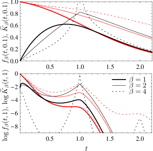
The peak appearing at $t=1$ for large $\lambda$ clearly indicates that here the correlations decay more slowly as a function of $\lambda$ than at all other times $t$. We study this in more detail by an asymptotic analysis in $\lambda$ of the exact integral expressions (7). We calculate the weight $W_{\beta}(t,\lambda)$ $=$ $\lambda^{2}\int_{t-\lambda^{-2}}^{t+\lambda^{-2}}\widetilde{K}_{\beta}(t^{\prime},\lambda)dt^{\prime}$ of the peaks at $t=1$ and, for the GSE, also at $t=2$. In contrast to the peak height the weight is well defined for all times for all three ensembles. We find

$$W_{\beta}(1,\lambda)\ \propto\ \lambda^{-2(4-\beta)/\beta}+{\cal O}(\lambda^{-8/\beta})$$ (8)

and $W_{4}(2,\lambda)\propto\lambda^{-6}$. The weight of the first peak $t\approx 0$ scales as $\lambda^{-2}$ independently of the ensemble. These decays are governed by power laws in $\lambda$ while they are exponential for all other times. We shall see below, that the behavior of the cross form-factor at $t=1$ is directly related to fidelity revivals, which for the GSE also occur at $t=2$.

For the classical ensembles $K_{\beta}(t)$, is non–analytic at $t=1$ Guhr et al. (1998). The degree $\mathcal{D}(g,x)$ of non–analyticity of a function $g(x)$ at $x$ is defined as the smallest integer $\mathcal{D}$ for which the $\mathcal{D}$-th derivative $g^{(\mathcal{D})}$ is discontinuous at $x$. For the form factor we find $\mathcal{D}(K_{4},1)=0$, $\mathcal{D}(K_{2},1)=1$ and $\mathcal{D}(K_{1},1)=\mathcal{D}(K_{4},2)=3$. For typical times we find $\mathcal{D}(K_{\beta},t)=\infty$, because $K_{\beta}(t)$ is analytic. We thus arrive at a relation between the asymptotic behavior of $W_{\beta}(t,\lambda)$ for large perturbation to the degree of non–analyticity of $K_{\beta}(t)$ which reads

$$W_{\beta}(t,\lambda)\ \propto\ \lambda^{-2\mathcal{D}(K_{\beta},t)}+\ldots\,,\ t>0\ .$$ (9)

We conjecture that this relation also holds for arbitrary $\beta\neq 1,2,4$.

We use the multiply kicked Ising (MKI) spin chain proposed in Prosen (2002); Pineda et al. (2006) to illustrate the revival in the cross form-factor. The MKI spin chain is a periodic 1-d array of $L$ spins $1/2$ with anti–ferromagnetic nearest–neighbor Ising interaction of unit strength and periodic boundary conditions. Each spin receives periodically two different kicks of instantaneous magnetic field pulses. The time–reversal breaking Floquet operator of the system is $U_{\text{MKI}}$ $=$ $U_{\text{I}}U_{\text{K}}^{(1)}U_{\text{I}}U_{\text{K}}^{(2)}$, where $U_{\text{I}}$ is the time evolution operator of the unkicked spin chain and $U_{\text{K}}^{(n)}=\exp(-\imath\sum_{j}\vec{b}^{(n)}\cdot\vec{\sigma}_{j})$, ($n=1,2$) describes each magnetic pulse with a dimensionless magnetic field $\vec{b}^{(n)}$. $\vec{\sigma}_{j}$ are the Pauli operators for particle $j$. The translational symmetry ($\vec{\sigma}_{j}\to\vec{\sigma}_{j+1}$) which foliates the space in $L$ different symmetry sectors. For the choice $\vec{b}^{(1)}=(0,1,1)$ and $\vec{b}^{(2)}=(1.4,0,1.4)$ the spectral statistics in most symmetry sectors display excellent agreement with the GUE. We introduce an additional magnetic pulse of strength $\delta$ in $z$ direction as a perturbation. We define $U_{\delta}=$ $U_{\text{MKI}}\cdot\exp\left(\imath\delta\sum_{j=0}^{L-1}\sigma^{z}_{j}\right)$ and calculate the cross form-factor of $U_{\text{MKI}}$ and $U_{\delta}$ using direct diagonalization, omitting the problematic sectors. The perturbation strength $\lambda$ can be calculated from $\delta$ using the correlation functions of the perturbing operator Gorin et al. (2006). Details are given elsewhere.

Figure 2: (Color online) The cross correlation function for the MKI model with $L=18$. Filled/empty triangles correspond to the real/imaginary part of the cross correlation. The statistical error (measured by the imaginary part) is small enough to observe clearly the peak. The theoretical expectation Eq. (7) is plotted as a thick curve.

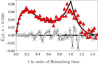
In Fig. 2 we compare results of this model with RMT results of Eq. (7). We see good agreement with the theoretical result, up to statistical fluctuations, measured by the imaginary part. In particular the peak at $t=1$ is observed.

We now derive the announced differential relations connecting the cross form–factor with fidelity, deferring the reader to a follow–up paper for more details. Consider a general 4-point parametric correlation function $F_{\alpha\beta;\gamma\delta}(z_{1},z_{2})=\left\langle\mathcal{F}_{\alpha\beta;\gamma\delta}(z_{1},z_{2};H^{-},H^{+})\right\rangle$ defined as

$$F_{\alpha\beta;\gamma\delta}(z_{1},z_{2})=\left\langle\left(\frac{1}{z_{1}-H^{-}}\right)_{\alpha\beta}\left(\frac{1}{z_{2}-H^{+}}\right)_{\gamma\delta}\right\rangle\ .$$ (10)

The definition of the angular brackets is now expanded to denote either the average over an arbitrary matrix ensemble with measure $d\nu(H)$, or the energy averaging over a spectral window of an individual quantum chaotic system. We do not require $d\nu(H)$ to be Gaussian or even rotationally invariant. The distribution of $V$, on the other hand, is required to be Gaussian in order to ensure the existence of the announced differential relations at finite order (see Eq. (16) below). The Fourier transform of fidelity amplitude corresponds to $F_{\alpha\beta;\beta\alpha}$ and parametric spectral correlator corresponds to $F_{\alpha\alpha;\beta\beta}$, with a summation over double indices. Introducing $H_{1,2}$ via $\delta(H_{1,2}-H^{\pm}(\lambda))$, Fourier transforming the matrix delta-functions and integrating over $V$, the averages are rewritten as

$$\left\langle\mathcal{F}\right\rangle=\int d\Lambda_{1}d\Lambda_{2}d\nu(H)dH_{1}dH_{2}$$

$$\quad e^{\mathrm{tr}\left[\imath\Lambda_{1}(H_{1}-H)+\imath\Lambda_{2}(H_{2}-H)-\frac{\lambda^{2}D^{2}}{4\beta}(\Lambda_{2}-\Lambda_{1})^{2}\right]}\,\mathcal{F}$$ (11)

where the symmetry class of the matrices $\Lambda_{1}$, $\Lambda_{2}$ corresponds to the symmetry class of $H$, and multiple factors of $2\pi$ are absorbed into the definition of $d\Lambda_{1,2}$ .

The invariance of the flat integration measures $dH_{1,2}$ with respect to independent shifts in $H_{1}$ and $H_{2}$ implies

$$\left\langle\mathrm{tr}\left(\frac{\partial}{\partial H_{1}}-\frac{\partial}{\partial H_{2}}\right)^{2}\mathcal{F}_{\alpha\alpha;\beta\beta}\right\rangle=-\left\langle\mathrm{tr}(\Lambda_{1}-\Lambda_{2})^{2}\mathcal{F}_{\alpha\alpha;\beta\beta}\right\rangle$$ (12)

The full measure in Eq. (Surprising relations between parametric level correlations and fidelity decay) is also approximately invariant under a simultaneous shift of $H_{1}$ and $H_{2}$. The violation of this symmetry stems from the non-invariance of $d\nu(H)$ under the shifts of $H$. However, universality implies that the correlation functions depend on such shifts only through the average density of states and level velocity variance sim . This dependence is thus manifested only on time scales much shorter than $t_{H}$, which is of interest here. In invariant unitary RMT ensembles universality under shifts was shown in smolyarenko . Although not yet proved in general, no violations of this universality are known. In particular universality follows automatically in models which allow for field theoretical representations of correlation functions Efetov (1996). With these caveats we can set

$$\left\langle\mathrm{tr}\left(\frac{\partial}{\partial H_{1}}+\frac{\partial}{\partial H_{2}}\right)^{2}\mathcal{F}_{\alpha\alpha;\beta\beta}\right\rangle\approx 0$$ (13)

and combine with Eq. (12) to

$$4\left\langle\mathrm{tr}\frac{\partial}{\partial H_{1}}\frac{\partial}{\partial H_{2}}\mathcal{F}_{\alpha\alpha;\beta\beta}\right\rangle=\left\langle\mathrm{tr}\left(\Lambda_{1}-\Lambda_{2}\right)^{2}\mathcal{F}_{\alpha\alpha;\beta\beta}\right\rangle\ .$$ (14)

Using

$$\left\langle\mathrm{tr}\frac{\partial}{\partial H_{1}}\frac{\partial}{\partial H_{2}}\mathcal{F}_{\alpha\alpha;\beta\beta}\right\rangle=\frac{\partial^{2}}{\partial z_{1}\partial z_{2}}F_{\alpha\beta;\beta\alpha},$$ (15)

$$\left\langle\mathrm{tr}(\Lambda_{1}-\Lambda_{2})^{2}\mathcal{F}_{\alpha\alpha;\beta\beta}\right\rangle=-\frac{4\beta}{D^{2}}\frac{\partial}{\partial\lambda^{2}}F_{\alpha\alpha;\beta\beta}$$ (16)

and Fourier transforming $F$, we finally show that

$$\frac{\partial}{\partial\lambda^{2}}\widetilde{K}_{\beta}(t,\lambda)=-\frac{4\pi^{2}t^{2}}{\beta}f_{\beta}(t,\lambda),$$ (17)

under very general assumptions. The averaged fidelity amplitude has been calculated in Ref. rud for the GOE and the GUE. For the GSE,

$$f_{4}(t,\lambda)=\int_{-1}^{+1}du\int_{0}^{1-|u|}dv\frac{(u+t)^{2}-1}{(t^{2}-v^{2})^{2}}|v|\theta(u-1+t)\\ \times\frac{(t^{2}-v^{2}+2tu)\exp\left(-\pi^{2}\lambda^{2}\left[t^{2}-v^{2}+2tu\right]\right)}{\sqrt{\left[(u-1)^{2}-v^{2}\right]\left[(u+1)^{2}-v^{2}\right]}}\ .$$ (18)

A direct comparison of the exact expressions for $\widetilde{K}_{\beta}(t,\lambda)$ obtained in the present contribution and of the ones for $f_{\beta}(t,\lambda)$ in Ref. rud and in Eq. (18) confirms the validity of Eq. (17) in the universal RMT regime (although we stress that it is valid for any disordered/chaotic model which exhibits a separation of scales between the oscillatory local and smooth global behavior of spectral statistics).

Relation (17) allows us to view fidelity revival at Heisenberg time $t_{H}$ as being rooted in the algebraic decay of the cross form-factor. Furthermore, due to the established relations, power law decay as a function of $\lambda$ must also hold for fidelity at $t_{H}$ and, for the GSE, at $2t_{H}$. This could also have been derived directly from the exact equations.

In Fig. 1, we show the fidelity amplitude. Similar to the behavior of the cross form-factor, a peak at $t=1$ appears for all three ensembles rud and for increasing $\beta$ the peaks become more and more pronounced. In the GSE case, a second peak emerges at $t=2$. This peak was not seen in the numerics of rud as it was beyond numerical accuracy.

Relation (17) is, essentially, a Ward identity associated with the action (Surprising relations between parametric level correlations and fidelity decay). It immediately allows to establish a connection between fidelity amplitude and the Fourier transform of the level velocity correlator $C(t,\lambda)$, which is related to $\widetilde{K}$ by a Ward identity $-4\pi^{2}t^{2}C(t,\lambda)=(\partial^{2}/\partial\lambda^{2})\widetilde{K}(t,\lambda)$ (see, e.g., lerner ). As seen from Eq. (Surprising relations between parametric level correlations and fidelity decay), $\widetilde{K}$ is a function of $\lambda^{2}$, it follows from (17) after a short calculation that

$$\beta C(t,\lambda)=\left(2+4\lambda^{2}\frac{\partial}{\partial\lambda^{2}}\right)f(t,\lambda)\ .$$ (19)

To summarize, we established relations between cross form-factor and level velocities on the one hand, and fidelity decay on the other hand. They hold in any system displaying universality of spectral correlations. The present formalism can be used to construct a whole family of Ward identities relating apparently unconnected correlation functions. One instance are generalizations of the ‘optical theorem’ found in taniguchi (2), which relates fidelity amplitude for small perturbations to the spectral form factor $K_{\beta}(t)$. Further, the results presented here do not apply to crossover regimes, where $V$ changes the symmetry of $H$. One such relation was obtained using supersymmetry methods in taniguchi (1). A broader set of differential relations, generalizing those of taniguchi (1), can be obtained by utilizing different transformation properties of the action Eq. (Surprising relations between parametric level correlations and fidelity decay) under symmetry-preserving and symmetry-violating shifts. Details of these and other hierarchies of relations will be presented elsewhere.

Our findings make it possible to explain features of one quantity via the other, i.e. the characteristics of fidelity decay in terms of the cross form-factor or vice versa. In particular, the revivals of both quantities are linked in this way. We studied in detail the decay laws of the corresponding peaks. Further peaks are not possible. The very occurrence of the peaks in the cross form-factors is neither trivial nor intuitive and will be discussed in elsewhere.