Dynamic probes of quantum spin chains
with the Dzyaloshinskii-Moriya interaction

Abstract

We consider the spin-$\frac{1}{2}$ anisotropic $XY$ chain in a transverse ($z$) field with the Dzyaloshinskii-Moriya interaction directed along $z$-axis in spin space to examine the effect of the Dzyaloshinskii-Moriya interaction on the $zz$, $xx$ and $yy$ dynamic structure factors. Using the Jordan-Wigner fermionization approach we analytically calculate the dynamic transverse spin structure factor. It is governed by a two-fermion excitation continuum. We analyze the effect of the Dzyaloshinskii-Moriya interaction on the two-fermion excitation continuum. Other dynamic structure factors which are governed by many-fermion excitations are calculated numerically. We discuss how the Dzyaloshinskii-Moriya interaction manifests itself in the dynamic properties of the quantum spin chain at various fields and temperatures.

1 Introduction. Jordan-Wigner representation

Recently the dynamic properties of quasi-one-dimensional quantum spin systems have become an intense area of research. On the one hand, a variety of quasi-one-dimensional materials were discovered during last decades. On the other hand, many exactly solvable statistical mechanics models refer to one spatial dimension. Very often these models permit to make a detailed analysis not only of their thermodynamic properties but also of their dynamic properties. Such theoretical investigations are necessary for interpretation of the experimental data observable in the scattering or resonance experiments on quasi-one-dimensional compounds [1].

In this paper we analyze the effect of the Dzyaloshinskii-Moriya interaction on the dynamic properties of quantum spin chains. The Dzyaloshinskii-Moriya interaction is present in many low-dimensional materials [2, 3, 4, 5, 6, 7, 8, 9, 10, 11, 12, 13, 14, 15]. Such antisymmetric exchange interaction, ${\bf D}_{{\bf{n}}{\bf{m}}}\cdot\left[{\bf{s}}_{\bf{n}}\times{\bf{s}}_{\bf{m}}\right]$, takes place, if allowed by crystal symmetry, due to spin-orbit coupling [16] and is weaker than the symmetric Heisenberg superexchange interaction $J_{{\bf{n}}{\bf{m}}}\left({\bf{s}}_{\bf{n}}\cdot{\bf{s}}_{\bf{m}}\right)$. In spite of this, this interaction has a number of important consequences and may cause a number of unconventional phenomena. Interestingly, the Dzyaloshinskii-Moriya interaction may appear while analyzing the nonequilibrium steady states of quantum spin chains with currents [17, 18, 19]. It may also appear in the quantum spin representation in the stochastic kinetics of adsorption-desorption processes [20] (see also [21]).

The analysis of the effect of the Dzyaloshinskii-Moriya interaction on the dynamic quantities of quantum spin chains was reported in several papers [22, 23]. In particular in Refs. [22, 23] such analysis was performed using the symmetry arguments and field-theoretical methods for the isotropic Heisenberg ($XXX$) chain.

In our study we restrict ourselves to a simpler model, i.e. anisotropic $XY$ chain, the dynamic properties of which are amenable to detailed analytical and numerical analysis. We should also note that Cs₂CoCl₄ provides a new example of spin-$\frac{1}{2}$ $XY$ chain [24] that may renew interest in the calculation of observable quantities for such a chain [25, 26, 27].

To be specific, we consider $N$ spins one-half governed by the following Hamiltonian

$$H=\sum_{n}\left(J^{x}s_{n}^{x}s_{n+1}^{x}+J^{y}s_{n}^{y}s_{n+1}^{y}\right)+\sum_{n}D\left(s_{n}^{x}s_{n+1}^{y}-s_{n}^{y}s_{n+1}^{x}\right)+\sum_{n}\Omega s_{n}^{z}.$$ (1.1)

Here $J^{x}$, $J^{y}$ are the anisotropic $XY$ exchange interaction constants, $D$ is the $z$-component of the Dzyaloshinskii-Moriya interaction and $\Omega$ is the transverse magnetic field. Such model was introduced in Refs. [28, 29]. Some of its dynamic properties were examined in Refs. [30, 31, 32, 33, 34]. In particular, the transverse dynamic susceptibility $\chi_{zz}(\kappa,\omega)$ of the model (1.1) was derived explicitly for $\kappa=0$ [30] and $\kappa\neq 0$ [32]. Moreover, the case of isotropic $XY$ interaction $J^{x}=J^{y}$ (in this case the Dzyaloshinskii-Moriya interaction can be eliminated from the Hamiltonian by a spin axes rotation) was analyzed in some detail [34, 35].

The performed analysis is based on the Jordan-Wigner transformation,

$$c_{1}=s_{1}^{-},\;\;\;c_{n}=\left(-2s_{1}^{z}\right)\left(-2s_{2}^{z}\right)\ldots\left(-2s_{n-1}^{z}\right)s_{n}^{-},\;n=2,\ldots,N,$$ (1.2)

which transforms (1.1) into the following bilinear Fermi form

$$H=\sum_{n}\left(\frac{J+{\mbox{i}}D}{2}c_{n}^{+}c_{n+1}-\frac{J-{\mbox{i}}D}{2}c_{n}c_{n+1}^{+}+\frac{\gamma}{2}\left(c_{n}^{+}c_{n+1}^{+}-c_{n}c_{n+1}\right)+\Omega\left(c_{n}^{+}c_{n}-\frac{1}{2}\right)\right)$$ (1.3)

with $J=\frac{1}{2}\left(J^{x}+J^{y}\right)$ and $\gamma=\frac{1}{2}\left(J^{x}-J^{y}\right)$.

In our calculations we consider both periodic and open boundary conditions. Of course, in the thermodynamic limit the results for bulk characteristics should be insensitive to the boundary conditions implied. In the former case, i.e. when $s_{N+1}^{\alpha}=s_{1}^{\alpha}$, the bilinear Fermi form (1.3) is periodic or antiperiodic depending on whether the number of fermions is odd or even. After the Fourier transformation,

$$c_{\kappa}=\frac{1}{\sqrt{N}}\sum_{n}\exp\left({\mbox{i}}\kappa n\right)c_{n},\;\;\;c_{n}=\frac{1}{\sqrt{N}}\sum_{\kappa}\exp\left(-{\mbox{i}}\kappa n\right)c_{\kappa}$$ (1.4)

(here $\kappa$ takes $N$ values $\frac{2\pi}{N}n$ for periodic boundary conditions or $\frac{2\pi}{N}\left(n+\frac{1}{2}\right)$ for antiperiodic boundary conditions; $n=-\frac{N}{2},-\frac{N}{2}+1,\ldots,\frac{N}{2}-1$ for $N$ even and $n=-\frac{N-1}{2},-\frac{N-1}{2}+1,\ldots,\frac{N-1}{2}$ for $N$ odd), and the Bogolyubov transformation with Fermi-operators $\beta$

$$\beta_{\kappa}={\mbox{i}}u_{\kappa}c_{\kappa}+v_{\kappa}c^{+}_{-\kappa},\;\;\;c_{\kappa}=-{\mbox{i}}u_{\kappa}\beta_{\kappa}+v_{\kappa}\beta^{+}_{-\kappa}$$ (1.5)

with

$$u_{\kappa}={\mbox{sgn}}\left(\gamma\sin\kappa\right)\frac{1}{\sqrt{2}}\sqrt{1+\frac{\Omega+J\cos\kappa}{\lambda_{\kappa}}},\;\;\;v_{\kappa}=\frac{1}{\sqrt{2}}\sqrt{1-\frac{\Omega+J\cos\kappa}{\lambda_{\kappa}}},$$

$$\lambda_{\kappa}=\sqrt{\left(\Omega+J\cos\kappa\right)^{2}+\gamma^{2}\sin^{2}\kappa}$$ (1.6)

the Hamiltonian (1.3) becomes

$$H=\sum_{\kappa}\Lambda_{\kappa}\left(\beta^{+}_{\kappa}\beta_{\kappa}-\frac{1}{2}\right),$$ (1.7)

$$\Lambda_{\kappa}=D\sin\kappa+\lambda_{\kappa}.$$ (1.8)

It should be noted here that only the energy spectrum $\Lambda_{\kappa}$ (1.8) but not the coefficients of the Bogolyubov transformation $u_{\kappa}$, $v_{\kappa}$ (1) depends on $D$. Using (1.8) one immediately finds that the energy spectrum is gapless when $\gamma^{2}\leq D^{2}$ and $\Omega^{2}\leq J^{2}+D^{2}-\gamma^{2}$ or when $\gamma^{2}>D^{2}$ and $\Omega^{2}=J^{2}$.

In our numerical calculations we use open boundary conditions [36]. The bilinear Fermi form (1.3) with open boundary conditions can be brought into the form (1.7) after a linear transformation

$$\eta_{k}=\sum_{j=1}^{N}\left(g_{kj}c_{j}+h_{kj}c_{j}^{+}\right),\;\;\;c_{j}=\sum_{k=1}^{N}\left(g_{kj}^{*}\eta_{k}+h_{kj}\eta_{k}^{+}\right)$$ (1.9)

where

$$\sum_{j=1}^{N}\left(g_{kj}A_{jm}-h_{kj}B_{jm}^{*}\right)=\Lambda_{k}g_{km},\;\;\;\sum_{j=1}^{N}\left(g_{kj}B_{jm}-h_{kj}A_{jm}^{*}\right)=\Lambda_{k}h_{km},$$

$$\sum_{j=1}^{N}\left(g_{kj}g_{qj}^{*}+h_{kj}h_{qj}^{*}\right)=\delta_{kq},\;\;\;\sum_{j=1}^{N}\left(g_{kj}g_{km}^{*}+h_{kj}^{*}h_{km}\right)=\delta_{jm},$$

$$\sum_{j=1}^{N}\left(g_{kj}h_{qj}+h_{kj}g_{qj}\right)=\sum_{k=1}^{N}\left(g_{kj}h_{km}^{*}+h_{kj}^{*}g_{km}\right)=0$$ (1.10)

with $A_{nm}=\Omega\delta_{nm}+\frac{1}{2}\left(J+{\mbox{i}}D\right)\delta_{m,n+1}+\frac{1}{2}\left(J-{\mbox{i}}D\right)\delta_{m,n-1}$, $B_{nm}=\frac{1}{2}\gamma\left(\delta_{m,n+1}-\delta_{m,n-1}\right)$. We are not aware of a general analytical solution for this problem. For the two particular cases, namely, the anisotropic $XY$ chain without field and the Ising chain in a transverse field such solutions can be found e.g. in Ref. [37]. In our study we solve Eqs. (1) numerically for chains of about a few hundred sites.

The relation between the spin model (1.1) and the noninteracting Jordan-Wigner fermions (1.7) is a key step in the statistical mechanics calculations for one-dimensional spin-$\frac{1}{2}$ $XY$ systems.

In our study of the dynamic properties we focus on the dynamic spin structure factors

$$S_{\alpha\alpha}(\kappa,\omega)=\frac{1}{N}\sum_{j=1}^{N}\sum_{n=1}^{N}\exp\left({\mbox{i}}\kappa n\right)\int_{-\infty}^{\infty}{\mbox{d}}t\exp\left({\mbox{i}}\omega t\right)\left(\langle s_{j}^{\alpha}(t)s_{j+n}^{\alpha}\rangle-\langle s_{j}^{\alpha}\rangle\langle s_{j+n}^{\alpha}\rangle\right),\;\;\;\alpha=x,y,z.$$ (1.11)

The dynamic structure factors are of considerable importance since they are directly comparable with inelastic neutron scattering experiments of some quasi-one-dimensional substances. The dynamic transverse spin structure factor $S_{zz}(\kappa,\omega)$ can be easily evaluated analytically (Section 2). The transverse dynamics is governed exclusively by a two-fermion excitation continuum the properties of which in the case of $XY$ chain without the Dzyaloshinskii-Moriya interaction were discussed earlier [38]. Another quantity which is also governed by the two-fermion excitation continuum is the dynamic dimer structure factor [39, 40, 41]. Therefore, the effect of the Dzyaloshinskii-Moriya interaction on the two-fermion excitation continuum deserves a separate discussion (Section 3). The $xx$ and $yy$ dynamic structure factors are computed numerically (Section 4). We compare and contrast the properties of different dynamic structure factors at different values of the transverse field and temperature emphasizing the effect of the Dzyaloshinskii-Moriya interactions. We end up with conclusions (Section 5).

Some preliminary results of this study were announced in the conference paper [42].

2 Dynamics of transverse spin correlations

We start with the $zz$ dynamic structure factor of the model (1.1). For analytical calculation of this quantity one can consider only periodic (or only antiperiodic) boundary conditions for the bilinear Fermi form (1.3). Using the relation between spin and Fermi operators (1.2) and the transformations (1.4) and (1.5), (1) after standard calculations using the Wick-Bloch-de Dominicis theorem we arrive at

$$S_{zz}(\kappa,\omega)=\int_{-\pi}^{\pi}{\mbox{d}}\kappa_{1}\left(\left(u_{\kappa_{1}}^{2}u_{\kappa_{1}-\kappa}^{2}-u_{\kappa_{1}}u_{\kappa_{1}-\kappa}v_{\kappa_{1}}v_{\kappa_{1}-\kappa}\right)n_{\kappa_{1}}\left(1-n_{\kappa_{1}-\kappa}\right)\delta\left(\omega+\Lambda_{\kappa_{1}}-\Lambda_{\kappa_{1}-\kappa}\right)\right.$$

$$\left.+\left(u_{\kappa_{1}}^{2}v_{\kappa_{1}-\kappa}^{2}+u_{\kappa_{1}}u_{\kappa_{1}-\kappa}v_{\kappa_{1}}v_{\kappa_{1}-\kappa}\right)n_{\kappa_{1}}n_{-\kappa_{1}+\kappa}\delta\left(\omega+\Lambda_{\kappa_{1}}+\Lambda_{-\kappa_{1}+\kappa}\right)\right.$$

$$\left.+\left(u_{\kappa_{1}-\kappa}^{2}v_{\kappa_{1}}^{2}+u_{\kappa_{1}}u_{\kappa_{1}-\kappa}v_{\kappa_{1}}v_{\kappa_{1}-\kappa}\right)\left(1-n_{-\kappa_{1}}\right)\left(1-n_{\kappa_{1}-\kappa}\right)\delta\left(\omega-\Lambda_{-\kappa_{1}}-\Lambda_{\kappa_{1}-\kappa}\right)\right.$$

$$\left.+\left(v_{\kappa_{1}}^{2}v_{\kappa_{1}-\kappa}^{2}-u_{\kappa_{1}}u_{\kappa_{1}-\kappa}v_{\kappa_{1}}v_{\kappa_{1}-\kappa}\right)\left(1-n_{-\kappa_{1}}\right)n_{-\kappa_{1}+\kappa}\delta\left(\omega-\Lambda_{-\kappa_{1}}+\Lambda_{-\kappa_{1}+\kappa}\right)\right)$$ (2.1)

where $n_{\kappa}=\left(\exp\left(\beta\Lambda_{\kappa}\right)+1\right)^{-1}$ is the Fermi function. This result agrees with the corresponding formula for the transverse dynamic susceptibility $\chi_{zz}(\kappa,\omega)$ derived in Ref. [32].

Introducing the function

$$f\left(\kappa_{1},\kappa\right)=\frac{\left(\Omega+J\cos\left(\kappa_{1}-\frac{\kappa}{2}\right)\right)\left(\Omega+J\cos\left(\kappa_{1}+\frac{\kappa}{2}\right)\right)-\gamma^{2}\sin\left(\kappa_{1}-\frac{\kappa}{2}\right)\sin\left(\kappa_{1}+\frac{\kappa}{2}\right)}{\lambda_{\kappa_{1}-\frac{\kappa}{2}}\lambda_{\kappa_{1}+\frac{\kappa}{2}}}$$ (2.2)

the dynamic structure factor $S_{zz}(\kappa,\omega)$ (2) can be expressed as follows

$$S_{zz}(\kappa,\omega)=\int_{-\pi}^{\pi}{\mbox{d}}\kappa_{1}\left(\frac{1+f\left(\kappa_{1},\kappa\right)}{2}\left(1-n_{\kappa_{1}-\frac{\kappa}{2}}\right)n_{\kappa_{1}+\frac{\kappa}{2}}\delta\left(\omega-\Lambda_{\kappa_{1}-\frac{\kappa}{2}}+\Lambda_{\kappa_{1}+\frac{\kappa}{2}}\right)\right.$$

$$\left.+\frac{1-f\left(\kappa_{1},\kappa\right)}{4}\left(\left(1-n_{\kappa_{1}-\frac{\kappa}{2}}\right)\left(1-n_{-\kappa_{1}-\frac{\kappa}{2}}\right)\delta\left(\omega-\Lambda_{\kappa_{1}-\frac{\kappa}{2}}-\Lambda_{-\kappa_{1}-\frac{\kappa}{2}}\right)\right.\right.$$

$$\left.\left.+n_{\kappa_{1}+\frac{\kappa}{2}}n_{-\kappa_{1}+\frac{\kappa}{2}}\delta\left(\omega+\Lambda_{\kappa_{1}+\frac{\kappa}{2}}+\Lambda_{-\kappa_{1}+\frac{\kappa}{2}}\right)\right)\right).$$ (2.3)

In the limit of isotropic $XY$ interaction $\gamma=0$ Eq. (2) yields the result obtained earlier [34]. In the limit $D=0$ (when $\Lambda_{\kappa}=\lambda_{\kappa}=\lambda_{-\kappa}\geq 0$) and $T=0$ ($\beta\to\infty$) Eq. (2) becomes

$$S_{zz}(\kappa,\omega)=\int_{-\pi}^{\pi}{\mbox{d}}\kappa_{1}\frac{1-f\left(\kappa_{1},\kappa\right)}{4}\delta\left(\omega-\Lambda_{\kappa_{1}-\frac{\kappa}{2}}-\Lambda_{\kappa_{1}+\frac{\kappa}{2}}\right).$$ (2.4)

This coincides with the expression obtained earlier in Ref. [38]. We notice that Eq. (2.4) is more generally valid for the case $\gamma^{2}>D^{2}$ (when $\Lambda_{\kappa}>0$) and $T=0$. In the case $D^{2}>\gamma^{2}$ and $T=0$ or in the most general case of arbitrary $D$ and $T>0$ (as well as in the case $D=0$ but $T>0$ which was not considered in Ref. [38]) the $zz$ dynamic structure factor exhibits new qualitative features in comparison with the analysis reported in Ref. [38]. Again the $zz$ dynamic structure factor is governed exclusively by two-fermion excitations as can be seen from Eq. (2), however, for $D^{2}>\gamma^{2}$, $T=0$ or for $T>0$ all three $\delta$-functions in Eq. (2) may come into play.

In Fig. 1 we show the gray-scale plots for $S_{zz}(\kappa,\omega)$ at low temperature ($\beta J=50$) for several typical sets of parameters ($J=1$, $\gamma=0.5$, $D=0,\;0.5,\;1$, $\Omega=0,\;0.5,\;1,\;\frac{\sqrt{7}}{2}$). For $\gamma^{2}>D^{2}$ (right column in Fig. 1) at such a low temperature only one two-fermion excitation continuum is relevant (the one which arises owing to $\delta\left(\omega-\Lambda_{\kappa_{1}-\frac{\kappa}{2}}-\Lambda_{-\kappa_{1}-\frac{\kappa}{2}}\right)$ in (2)) whereas in the opposite case $D^{2}>\gamma^{2}$ (left column in Fig. 1) all three two-fermion excitation continua contribute to transverse dynamics. In Fig. 2 we demonstrate typical low-temperature frequency profiles of $S_{zz}(0,\omega)$, $S_{zz}(\frac{\pi}{2},\omega)$, $S_{zz}(\pi,\omega)$ for a chain with $J=1$, $\gamma=0.5$, $\Omega=0.5$ and different values of the Dzyaloshinskii-Moriya interaction $D=0,\;0.5,\;1$. In Fig. 3 we show the gray-scale plots for $S_{zz}(\kappa,\omega)$ at intermediate and high temperatures ($\beta J=10,\;1,\;0.1$) for a chain with $J=1$, $\gamma=0.5$, $D=1$, $\Omega=0.5$. All these data are used herein to discuss generic properties of a two-fermion dynamic structure factor (Section 3) and to compare different dynamic structure factors (Section 4).

3 Two-fermion excitation continua

The $zz$ dynamic structure factor (2) can be rewritten in the form

$$S_{zz}(\kappa,\omega)=\sum_{j=1}^{3}S_{zz}^{(j)}(\kappa,\omega),\;\;\;S_{zz}^{(j)}(\kappa,\omega)=\int_{-\pi}^{\pi}{\mbox{d}}\kappa_{1}B^{(j)}(\kappa_{1},\kappa)C^{(j)}(\kappa_{1},\kappa)\delta\left(\omega-E^{(j)}(\kappa_{1},\kappa)\right)$$ (3.1)

with

$$B^{(1)}(\kappa_{1},\kappa)=B^{(3)}(\kappa_{1},\kappa)=\frac{1-f(\kappa_{1},\kappa)}{4},$$

$$B^{(2)}(\kappa_{1},\kappa)=\frac{1+f(\kappa_{1},\kappa)}{2},$$ (3.2)

$$C^{(1)}(\kappa_{1},\kappa)=\left(1-n_{\kappa_{1}-\frac{\kappa}{2}}\right)\left(1-n_{-\kappa_{1}-\frac{\kappa}{2}}\right),$$

$$C^{(2)}(\kappa_{1},\kappa)=\left(1-n_{\kappa_{1}-\frac{\kappa}{2}}\right)n_{\kappa_{1}+\frac{\kappa}{2}},$$

$$C^{(3)}(\kappa_{1},\kappa)=n_{\kappa_{1}+\frac{\kappa}{2}}n_{-\kappa_{1}+\frac{\kappa}{2}},$$ (3.3)

$$E^{(1)}(\kappa_{1},\kappa)=\Lambda_{\kappa_{1}-\frac{\kappa}{2}}+\Lambda_{-\kappa_{1}-\frac{\kappa}{2}},$$

$$E^{(2)}(\kappa_{1},\kappa)=\Lambda_{\kappa_{1}-\frac{\kappa}{2}}-\Lambda_{\kappa_{1}+\frac{\kappa}{2}},$$

$$E^{(3)}(\kappa_{1},\kappa)=-\Lambda_{\kappa_{1}+\frac{\kappa}{2}}-\Lambda_{-\kappa_{1}+\frac{\kappa}{2}}.$$ (3.4)

In accordance with (3.1) we distinguish three two-fermion excitation continua (they correspond to $j=1,2,3$ in Eq. (3.1)) which govern $S_{zz}(\kappa,\omega)$. The gray-scale plots of $S_{zz}^{(j)}(\kappa,\omega)$, $j=1,2,3$ for a typical set of parameters, $J=1$, $\gamma=0.5$, $D=1$, $\Omega=0.5$, $\beta=50$, are shown in Fig. 4. As can be seen from (3.1) and (3), (3), (3) the specific features of the considered two-fermion dynamic structure factor which describes the dynamics of the transverse spin fluctuations are controlled by the $B^{(j)}$-functions. Therefore, in Fig. 5 we also plot $S_{zz}^{(j)}(\kappa,\omega)$ (3.1) for the same set of parameters as in Fig. 4, although, with $B^{(j)}(\kappa_{1},\kappa)=1$. By comparing Figs. 4 and 5 one can distinguish the specific features (coming from the $B^{(j)}$-functions (3)) and the generic features (coming from the $C^{(j)}$-functions (3) and the $E^{(j)}$-functions (3)) of the dynamic quantity considered (see discussion below).

We remark that although we were not able to find a simple analytical form of the most important lines in the $\kappa$–$\omega$ plane characterizing the two-fermion excitation continua for a general case of the spin chain (1.1) it is easy to determine these functions numerically for any set of parameters using MAPLE or/and FORTRAN codes. We also recall that in the simplest case of the isotropic $XY$ model in a transverse field ($\gamma=0$, $D=0$) the corresponding results have been derived analytically [43]. However, in the case $\gamma\neq 0$, $D=0$ the analytical results have been reported only in the limiting cases $\Omega=0$ or $\gamma=1$ [38]. Of course, the case $\gamma\neq 0$, $D\neq 0$ considered in the present paper is even more complicated. In what follows we take a typical set of parameters $J=1$, $\gamma=0.5$, $D=1$, $\Omega=0.5$.

We begin with the case of infinite temperature $T\to\infty$ ($\beta=0$). The two-fermion dynamic structure factor may have nonzero values in the plane wave-vector $\kappa$ – frequency $\omega$ if the equation

$$\omega-E^{(j)}(\kappa_{1},\kappa)=0$$ (3.5)

has at least one solution $\kappa_{1}^{\star}$, $-\pi\leq\kappa_{1}^{\star}<\pi$. In Fig. 6 (panels a ($j=1$), b ($j=2$), c ($j=3$)) we show the regions in the $\kappa$–$\omega$ plane in which equation (3.5) has four solutions (dark-gray regions), two solutions (gray regions) or has no solutions (white regions). The bounding lines of the regions in which equation (3.5) has solutions constitute the upper ($\omega^{(j)}_{u}(\kappa)$) and the lower ($\omega^{(j)}_{l}(\kappa)\leq\omega^{(j)}_{u}(\kappa)$) boundaries of the two-fermion excitation continuum, respectively; moreover, for some regions of the wave-vector $\kappa$ the lower boundaries $\omega^{(j)}_{l}(\kappa)$ may be equal to zero. Alternatively, we may find the upper and the lower boundaries of the two-fermion excitation continuum seeking for the maximal and minimal values of $E^{(j)}(\kappa_{1},\kappa)$ while $\kappa_{1}$ varies from $-\pi$ to $\pi$, i.e.,

$$\omega^{(j)}_{u}(\kappa)=\max_{-\pi\leq\kappa_{1}<\pi}\left\{E^{(j)}(\kappa_{1},\kappa)\right\},\;\;\;\omega^{(j)}_{l}(\kappa)=\min_{-\pi\leq\kappa_{1}<\pi}\left\{0,\;E^{(j)}(\kappa_{1},\kappa)\right\}.$$ (3.6)

We have found that $\omega^{(j)}_{u}(\kappa)$ and $\omega^{(j)}_{l}(\kappa)\neq 0$ occur for the values of $\kappa_{1}$, $\kappa_{1}^{\star}$, which satisfy the equation

$$\left.\frac{\partial}{\partial\kappa_{1}}E^{(j)}(\kappa_{1},\kappa)\right|_{\kappa_{1}=\kappa_{1}^{\star}}=0.$$ (3.7)

Moreover, Eq. (3.7) also holds along the boundary $\omega(\kappa)$ between the gray and the dark-gray regions in the upper ($j=1$) and the middle ($j=2$) panels in the left column in Fig. 6. On the other hand, the quantities

$$S^{(j)}(\kappa,\omega)=\int_{-\pi}^{\pi}{\mbox{d}}\kappa_{1}{\cal{S}}^{(j)}(\kappa_{1},\kappa)\delta\left(\omega-E^{(j)}(\kappa_{1},\kappa)\right)=\sum_{\left\{\kappa_{1}^{\star}\right\}}\left.\frac{{\cal{S}}^{(j)}(\kappa_{1},\kappa)}{\left|\frac{\partial}{\partial\kappa_{1}}E^{(j)}(\kappa_{1},\kappa)\right|}\right|_{\kappa_{1}=\kappa_{1}^{\star}},$$ (3.8)

where $\left\{\kappa_{1}^{\star}\right\}$ are solutions of Eq. (3.5), may exhibit a van Hove singularity along the line $\omega^{(j)}_{s}(\kappa)=E^{(j)}(\kappa_{1}^{\star},\kappa)$, where $\kappa_{1}^{\star}$ satisfies Eq. (3.7). Thus, the mentioned boundary lines in the panels in the left column in Fig. 6 are the lines of van Hove singularities akin to the density of states effect in one dimension. Further, we have found that for almost all cases $\frac{\partial^{2}}{{\partial\kappa_{1}}^{2}}E^{(j)}(\kappa_{1},\kappa)\neq 0$ for the values of $\kappa_{1}$ which satisfy (3.5) with $\omega=\omega^{(j)}_{s}(\kappa)$ that obviously implies a familiar square-root divergence

$$S^{(j)}(\kappa,\omega)\propto\epsilon^{-\frac{1}{2}}$$ (3.9)

when $\omega$ approaches $\omega^{(j)}_{s}(\kappa)$, $\epsilon=\left|\omega-\omega^{(j)}_{s}(\kappa)\right|$. However, for $j=2$ and $\kappa\approx 1.07844531$ (see panel b in Fig. 6) Eq. (3.7) holds for $\kappa_{1}\approx 2.16480069$ and at this point $\frac{\partial^{2}}{{\partial\kappa_{1}}^{2}}E^{(2)}(\kappa_{1},\kappa)=0$ but $\frac{\partial^{3}}{{\partial\kappa_{1}}^{3}}E^{(2)}(\kappa_{1},\kappa)\approx 2.96548741\neq 0$. As a result, if $\omega$ is in the $\epsilon$-vicinity of $\omega^{(2)}_{s}(\kappa\approx 1.07844531)\approx 0.78594502$ the quantity $S^{(2)}(\kappa,\omega)$ (3.8) exhibits singularity with another exponent

$$S^{(2)}(\kappa\approx 1.07844531,\omega\approx 0.78594502\pm\epsilon)\propto\epsilon^{-\frac{2}{3}}.$$ (3.10)

We illustrate different types of singularities in Fig. 7. In particular, in Fig. 7a one can see the square-root divergencies (3.9), whereas in Fig. 7b aside from the square-root divergences (3.9) (solid and dotted curves) one can also see the dependence (3.10) (dashed curve). We notice that the $\epsilon^{-\frac{2}{3}}$ singularity remains for other values of $D$ and is also present when $D\to 0$. For $J=1$, $\gamma=0.5$, $D=0$, $\Omega=0.5$ it occurs at $\kappa\approx 1.68213734$ while $\omega$ approaches $\omega_{s}^{(2)}(\kappa\approx 1.68213734)=0$. Interestingly, this fact could not be detected in the earlier study on the $zz$ dynamics in the anisotropic $XY$ chain in a transverse field without the Dzyaloshinskii-Moriya interaction [38] since that study refers to the zero-temperature case when only the continuum $j=1$ manifests itself in the transverse spin dynamics (see discussion after Eq. (2.4)). We also notice that the observation of the $\epsilon^{-\frac{2}{3}}$ singularity may be difficult because of the fact that this peculiarity takes place only at one specific value of $\kappa$ (in contrast to the $\epsilon^{-\frac{1}{2}}$ singularity). However, for the values of wave-vector in the vicinity of this specific value one easily distinguishes a reminiscence of the $\epsilon^{-\frac{2}{3}}$ singularity (see the dotted curve in Fig. 7b). Finally we note that for some of the lines characterizing the two-fermion excitation continua we can give simple analytical expressions. Thus, for $j=1$ the maximum/minimum of $E^{(j)}(\kappa_{1},\kappa)$ occurs at $\kappa_{1}=0$ and $\kappa_{1}=-\pi$ and hence the corresponding boundary lines are given by $E^{(1)}(0,\kappa)$ and $E^{(1)}(-\pi,\kappa)$. We did not find simple analytical expressions for the boundary lines between the white and the dark-gray regions and for the nonzero lower boundary (see panel a in Fig. 6). For $j=3$ the upper boundary is given by $E^{(3)}(0,\kappa)$ and $E^{(3)}(-\pi,\kappa)$.

Next we turn to the zero-temperature case $T=0$ ($\beta\to\infty$) for which the effect of the Fermi functions involved in $C^{(j)}$-functions becomes important. The Fermi functions contract a region of possible values of $\kappa_{1}$ in Eq. (3.5); now $\kappa_{1}$ varies only within a part of the region between $-\pi$ and $\pi$ where $C^{(j)}(\kappa_{1},\kappa)\neq 0$. In Fig. 6 (panels d ($j=1$), e ($j=2$), f ($j=3$)) we show the regions in the $\kappa$–$\omega$ plane in which Eq. (3.5) taking into account the condition $C^{(j)}(\kappa_{1},\kappa)\neq 0$ has four solutions (dark-gray regions in panel d), two solutions (gray regions), one solution (light-gray regions in panel e) or has no solutions (white regions). The upper and the lower boundaries may be also found according to Eq. (3.6), although with $\kappa_{1}$ varying within a part of the region between $-\pi$ and $\pi$ where $C^{(j)}(\kappa_{1},\kappa)\neq 0$. The values of $\kappa$ at which $\omega^{(j)}_{l}(\kappa)=0$ correspond to the potential soft modes $\kappa_{c}$ (see the right panels in Fig. 6). (Note that the soft modes may not occur owing to $B^{(j)}$-functions (compare Figs. 4 and 5).) The two-fermion dynamic quantities may exhibit the above discussed van Hove singularities if their occurrence is not prohibited by the Fermi functions (and $B^{(j)}$-functions, compare Figs. 4 and 5). Moreover, along the bounding lines between the regions of $\kappa$–$\omega$ plane corresponding to different numbers of solution of Eq. (3.5) the two-fermion dynamic quantities may abruptly change their values exhibiting a finite jump (for example, we refer to the boundary line between the gray and light-gray regions in Fig. 6e; see also the panels b in Figs. 4 and 5). We can write down the analytical expressions for some characteristic lines seen in Figs. 6d, 6e, 6f. We introduce

$$\cos\kappa_{\pm}=\frac{-\Omega J\pm\sqrt{\left(D^{2}-\gamma^{2}\right)\left(J^{2}+D^{2}-\gamma^{2}-\Omega^{2}\right)}}{J^{2}+D^{2}-\gamma^{2}},\;\;\;D\sin\kappa_{\pm}<0;$$ (3.11)

$\kappa_{\pm}$ obey the equation $\Lambda_{\kappa_{\pm}}=0$. For the chosen set of parameters $J=1$, $\gamma=0.5$, $D=1$, $\Omega=0.5$ we have $\kappa_{+}\approx-1.24466864$, $\kappa_{-}\approx-2.67211739$. The lines $\Lambda_{-\kappa_{\pm}-\kappa}$ form the lower boundary of the continuum $j=1$; the lines $\Lambda_{\kappa_{\pm}-\kappa}$, $-\Lambda_{\kappa_{\pm}+\kappa}$ form the lower boundary of the continuum $j=2$; the lines $-\Lambda_{\kappa-\kappa_{\pm}}$ form the lower boundary of the continuum $j=3$. The soft modes may occur at the values of wave-vector $-2\kappa_{\pm},\;-\kappa_{+}-\kappa_{-}$ ($j=1$), $0,\;\pm\left(\kappa_{+}-\kappa_{-}\right)$ ($j=2$), $2\kappa_{\pm},\;\kappa_{+}+\kappa_{-}$ ($j=3$).

Finally, we emphasize a role of $B^{(j)}$-functions (3) which are responsible for the specific features of the dynamic transverse spin structure factor $S_{zz}(\kappa,\omega)$. The functions $B^{(j)}(\kappa_{1},\kappa)$ modify and add some additional structure to $S_{zz}(\kappa,\omega)$ in the $\kappa$–$\omega$ plane (compare Fig. 4 and Figs. 5, 6d, 6e, 6f referring to the low-temperature limit and Fig. 3c and Figs. 6a, 6b, 6c referring to the high-temperature limit). In particular, the function $B^{(2)}(\kappa_{1},\kappa)$ removes the soft modes at $\kappa=\pm\left(\kappa_{+}-\kappa_{-}\right)$ but not at $\kappa=0$ from $S_{zz}(\kappa,\omega)$ (see Fig. 4b). Furthermore, comparing Figs. 4a, 4c and 5a, 5c one sees that van Hove singularities along the lines $\omega=E^{(1)}(0,\kappa)$, $\omega=E^{(1)}(-\pi,\kappa)$ (panels a) and along the lines $\omega=E^{(3)}(0,\kappa)$, $\omega=E^{(3)}(-\pi,\kappa)$ (panels c) disappear since $B^{(1)}(0,\kappa)=B^{(3)}(0,\kappa)=B^{(1)}(-\pi,\kappa)=B^{(3)}(-\pi,\kappa)=0$.

To summarize this Section, the two-fermion dynamic structure factors have a nonzero value only in a restricted area of the $\kappa$–$\omega$ plane (two-fermion excitation continua) and may exhibit the van Hove singularities not only with exponent $\frac{1}{2}$ but also with exponent $\frac{2}{3}$. Moreover, at zero temperature the two-fermion dynamic structure factors may exhibit jumps at which their values abruptly increase by a finite value.

4 $xx$ and $yy$ dynamic structure factors

In the present Section we calculate the $xx$ and $yy$ dynamic structure factors. For numerical calculations it is convenient to rewrite (1.11) in the following form

$$S_{\alpha\alpha}(\kappa,\omega)=\int_{-\infty}^{\infty}{\mbox{d}}t\exp\left({\mbox{i}}\omega t\right)\left(\langle s_{j}^{\alpha}(t)s_{j}^{\alpha}\rangle-\langle s^{\alpha}\rangle^{2}\right)$$

$$+2\sum_{n=1,2,3,\ldots}\int_{-\infty}^{\infty}{\mbox{d}}t\;{\mbox{Re}}\left(\exp\left({\mbox{i}}\kappa n\right)\exp\left({\mbox{i}}\omega t\right)\left(\langle s_{j}^{\alpha}(t)s_{j+n}^{\alpha}\rangle-\langle s^{\alpha}\rangle^{2}\right)\right)$$ (4.1)

(we have omitted $\frac{1}{N}\sum_{j=1}^{N}$ in (1.11) and have used the relation $\langle s_{j}^{\alpha}(-t)s_{j+n}^{\alpha}\rangle=\langle s_{j}^{\alpha}(t)s_{j-n}^{\alpha}\rangle^{\star}$). As a result, to get $S_{\alpha\alpha}(\kappa,\omega)$ according to (4) we have to compute the time-dependent spin correlation functions $\langle s_{j}^{\alpha}(t)s_{j+n}^{\alpha}\rangle$, $n=0,1,2,\ldots$ with $t$ varying from $-\infty$ to $\infty$. We compute $\left\langle s_{j}^{\alpha}(t)s_{j+n}^{\alpha}\right\rangle$ $\alpha=x,y$ numerically. For this purpose we express the spin operators entering the time-dependent correlation functions in terms of auxiliary operators $\varphi_{l}^{\pm}=c_{l}^{+}\pm c_{l}$ which according to Eq. (1.9) are linear combinations of operators $\eta_{k}^{+}$, $\eta_{k}$. Since the $x$ and $y$ spin components at each site are essentially nonlocal objects in terms of Jordan-Wigner fermions (see (1.2)) the resulting expressions for the time-dependent spin correlation functions $\langle s_{j}^{\alpha}(t)s_{j+n}^{\alpha}\rangle$, $\alpha=x,y$ are complicated averages of products of a large number of Fermi operators attached not only the sites $j$ and $j+n$ but to two strings of sites extending to the boundary of the chain. After applying the Wick-Bloch-de Dominicis theorem one gets an intricate result which can be compactly written as the Pfaffian of the $2(2j+n-1)\times 2(2j+n-1)$ antisymmetric matrix constructed from elementary contractions $\langle\varphi_{l}^{+}(t)\varphi^{+}_{m}\rangle$, $\langle\varphi_{l}^{+}(t)\varphi^{-}_{m}\rangle$, $\langle\varphi_{l}^{-}(t)\varphi^{+}_{m}\rangle$, $\langle\varphi_{l}^{-}(t)\varphi^{-}_{m}\rangle$. The elementary contractions are easily expressed in terms of $\Lambda_{k}$, $g_{kj}$, $h_{kj}$ (1.9), (1). Finally we numerically evaluate the Pfaffians. Typically we take $N=400$, assume $j=31,\;71,\;131$ and calculate the correlation functions with $n$ up to $50,\;70,\;140$ in the time range $-50\div 50,\;-100\div 100,\;-300\div 300,\;-600\div 600$. To remove the effect of a finite time cut-off we multiply the integrands in (4) by $\exp\left(-{\rm{i}}\epsilon|t|\right)$ with $\epsilon=0.01,\;0.02$. To be sure that our results pertain to the thermodynamic limit we examine in detail different types of finite size effects (for further details see Refs. [36]).

In Fig. 8 (Fig. 9) we plot $S_{xx}(\kappa,\omega)$ ($S_{yy}(\kappa,\omega)$) at low temperature ($\beta J=50$) for several typical sets of parameters ($J=1$, $\gamma=0.5$, $D=0,\;0.5,\;1$, $\Omega=0,\;0.25,\;0.5,\;1$). (For larger values of the transverse field $\Omega$ there are no qualitative changes in these dynamic structure factors: they have a simple single-mode structure.) In Fig. 10 (Fig. 11) we show typical low-temperature frequency profiles of $S_{xx}(\kappa,\omega)$ ($S_{yy}(\kappa,\omega)$) at $\kappa=0$, $\kappa=\frac{\pi}{2}$, $\kappa=\pi$ for a chain with $J=1$, $\gamma=0.5$, $\Omega=0.5$ and different values of the Dzyaloshinskii-Moriya interaction $D=0,\;0.5,\;1$. In Fig. 12 (Fig. 13) we plot $S_{xx}(\kappa,\omega)$ ($S_{yy}(\kappa,\omega)$) at intermediate and high temperatures ($\beta J=10,\;1,\;0.1$) for a chain with $J=1$, $\gamma=0.5$, $D=1$, $\Omega=0.5$.

In contrast to transverse dynamic structure factor, the $xx$ and $yy$ dynamic structure factors are essentially more complicated quantities within the Jordan-Wigner method. Really, owing to a nonlocal relation between the $x$ and $y$ spin components and Fermi operators (1.2) the $xx$ and $yy$ time-dependent spin correlation functions are expressed through many-particle correlation functions of noninteracting Jordan-Wigner fermions. Let us now discuss the obtained numerical results. First of all we note that both dynamic structure factors $S_{xx}(\kappa,\omega)$ and $S_{yy}(\kappa,\omega)$ show similar behavior for the taken value of $\gamma=0.5$; obviously they become identical in the isotropic limit $\gamma=0$. We start with the dynamic structure factors at low temperatures. As can be seen in Figs. 8 and 9 (and Figs. 12a and 13a) these dynamic structure factors show several washed-out excitation branches which are roughly in correspondence with the characteristic lines of the two-fermion excitation continua (compare three dynamic structure factors in the panel a and the panels b and c in Fig. 14; note that these quantities are shown for $\kappa$ that varies from $-\pi$ to $3\pi$). Thus, although $S_{xx}(\kappa,\omega)$ and $S_{yy}(\kappa,\omega)$ are many-particle quantities within the Jordan-Wigner picture and hence they are not restricted to some region in the $\kappa$–$\omega$ plane, their values outside the two-fermion continua are rather small. This observation (i.e. two-particle features dominate many-particle dynamic quantities $S_{xx}(\kappa,\omega)$ and $S_{yy}(\kappa,\omega)$ at low temperatures) agrees with our previous studies on isotropic $XY$ chains [36, 34] (see also Ref. [38]). The constant frequency scans for several values of the wave-vector displayed in Figs. 10, 11 show the redistribution of spectral weight $S_{xx}(\kappa,\omega)$ and $S_{yy}(\kappa,\omega)$ as the Dzyaloshinskii-Moriya interaction $D$ increases. We note that these frequency profiles exhibit one or several peaks that may be relatively sharp or broad. The Dzyaloshinskii-Moriya interaction affects the positions of the peaks, their shapes and even their number (see, for example, the dependences $S_{xx}(0,\omega)$ vs $\omega$ and $S_{yy}(0,\omega)$ vs $\omega$ displayed in Figs. 10a and 11a). Constant frequency (and wave-vector) scans can be obtained for quasi-one-dimensional compounds by neutron scattering or resonance techniques and our findings may be useful in explaining the experimental data for the corresponding materials. As can be seen from our results, the Dzyaloshinskii-Moriya interaction clearly manifests itself in the frequency or wave-vector profiles of the dynamic structure factors that can be used in determining the magnitude of this interaction.

It should be remarked that the dynamic structure factors of quantum spin chains are often examined within the framework of a bosonization approach [44, 23]. Note, however, that field-theoretical approaches do not apply to small length scales and short time scales when the discreteness of the lattice becomes important. Therefore, since these methods can describe only the low-energy physics, the high-frequency features nicely seen in Figs. 8 and 9 cannot be reproduced by these theories.

As temperature increases, the low-temperature structure gradually disappears and the dynamic structure factors $S_{xx}(\kappa,\omega)$ and $S_{yy}(\kappa,\omega)$ become $\kappa$-independent in the high-temperature limit (see Figs. 12 and 13). This is in agreement with earlier studies in the infinite temperature limit [31].

To summarize, $xx$ and $yy$ dynamic structure factors at low temperatures are not restricted to the two-fermion excitation continua and have (small) nonzero values outside these continua. They exhibit several washed-out excitations concentrated along the characteristic lines of the two-fermion excitation continua. The Dzyaloshinskii-Moriya interaction manifests itself in the constant frequency/wave-vector scans influencing the detailed structure of such profiles. In the high-temperature limit $xx$ and $yy$ dynamic structure factors become $\kappa$-independent.

5 Conclusions

In this paper, we have obtained the detailed dynamic structure factors $S_{\alpha\alpha}(\kappa,\omega)$, $\alpha=x,y,z$ of the spin-$\frac{1}{2}$ anisotropic $XY$ chain in a transverse field with the Dzyaloshinskii-Moriya interaction. The Dzyaloshinskii-Moriya interaction leads to nontrivial changes in the dynamic quantities. The two-fermion excitations which exclusively govern the $zz$ dynamic structure factor, form three excitation continua and all of them manifest themselves even at zero temperature for sufficiently large strength of the Dzyaloshinskii-Moriya interaction. The two-fermion dynamic quantities have nonzero values in a restricted region of the $\kappa$–$\omega$ plane; they may exhibit van Hove singularities (not only with exponent $\frac{1}{2}$ but also with $\frac{2}{3}$); moreover, they may exhibit finite jumps at zero temperature. The $xx$ and $yy$ dynamic structure factors involve many-fermion excitations. However, the two-fermion excitations dominate their low-temperature behavior: at low temperatures these quantities show several washed-out excitation branches which correspond to specific lines of the two-fermion excitation continua.

The Dzyaloshinskii-Moriya interaction clearly manifests itself in the frequency/wave-vector profiles which makes it possible to determine the magnitude of this interaction by measuring the dynamic structure factors. Dynamical structure factors can be measured by neutron scattering. Another experimental technique which yields dynamic quantities is electron spin resonance (ESR). If a static magnetic field along $z$ axis and the electromagnetic wave polarized in $\alpha\perp z$ direction are applied to the spin-$\frac{1}{2}$ anisotropic $XY$ chain with the Dzyaloshinskii-Moriya interaction, the experimentally measurable absorption intensity is given by

$$I(\omega)\propto\omega\frac{1-\exp\left(-\beta\omega\right)}{2}S_{\alpha\alpha}(0,\omega).$$ (5.1)

Thus, the theoretical results for the dynamic structure factors presented in Section 4 are directly related to the ESR absorption intensity $I(\omega)$ (5.1). Similar study for the spin-$\frac{1}{2}$ isotropic $XY$ chain has been recently reported in Ref. [45]. A detailed analysis of the Dzyaloshinskii-Moriya interaction effect on ESR experiments on the materials, which can be modeled by the spin-$\frac{1}{2}$ anisotropic $XY$ chain, seems to be an interesting issue. The work in this direction is in progress.

FIGURE CAPTIONS

FIG. 1. Gray-scale plot for the $zz$ dynamic structure factor $S_{zz}(\kappa,\omega)$ (2) for the spin chain (1.1) with $J=1$, $\gamma=0.5$ at low temperature, $\beta=50$, for different strengths of the Dzyaloshinskii-Moriya interaction, $D=0$ (right column), $D=0.5$ (middle column), $D=1$ (left column), and different fields, $\Omega=0,\;0.5,\;1,\;\frac{\sqrt{7}}{2}$ (from bottom to top).

FIG. 2. Frequency profiles of $S_{zz}(\kappa,\omega)$ at different wave-vectors $\kappa=0$ (left panel), $\kappa=\frac{\pi}{2}$ (middle panel) and $\kappa=\pi$ (right panel) for the spin chain (1.1) with $J=1$, $\gamma=0.5$, $D=0$ (dotted lines), $D=0.5$ (dashed lines), $D=1$ (solid lines), $\Omega=0.5$ at low temperature $\beta=50$.

FIG. 3. The $zz$ dynamic structure factor (2) for the spin chain (1.1) with $J=1$, $\gamma=0.5$, $D=1$, $\Omega=0.5$ at different temperatures $\beta=10$ (a), $\beta=1$ (b) and $\beta=0.1$ (c).

FIG. 4. The gray-scale plots of $S_{zz}^{(1)}(\kappa,\omega)$ (a), $S_{zz}^{(2)}(\kappa,\omega)$ (b) and $S_{zz}^{(3)}(\kappa,\omega)$ (c) for the set of parameters $J=1$, $\gamma=0.5$, $D=1$, $\Omega=0.5$, $\beta=50$.

FIG. 5. For comparison $S_{zz}^{(j)}(\kappa,\omega)$ (3.1) with $B^{(j)}(\kappa_{1},\kappa)=1$ for the same set of parameters as in Fig. 4. a: $j=1$, b: $j=2$, c: $j=3$.

FIG. 6. Towards the properties of the two-fermion excitation continua; $J=1$, $\gamma=0.5$, $D=1$, $\Omega=0.5$; left panels – infinite temperature limit $T\to\infty$ ($\beta=0$), right panels – zero temperature limit $T=0$ ($\beta\to\infty$); $j=1$ (panels a and d), $j=2$ (panels b and e), $j=3$ (panels c and f).

FIG. 7. Frequency profiles (3.8) (with ${\cal{S}}^{(j)}(\kappa_{1},\kappa)=1$) for the chain (1.1) with $J=1$, $\gamma=0.5$, $D=1$, $\Omega=0.5$, $\beta=0$ which illustrate van Hove singularities with different exponents $\frac{1}{2}$ and $\frac{2}{3}$. Panel a: $S^{(1)}(\kappa,\omega)$ (3.8) vs $\omega$ at $\kappa=0.5$ (solid line), $\kappa=2$ (dashed line), $\kappa=3$ (dotted line); panel b: $S^{(2)}(\kappa,\omega)$ (3.8) vs $\omega$ at $\kappa=0.9$ (solid line), $\kappa\approx 1.07844531$ (dashed line; the low-frequency singularity has power-law exponent $\frac{2}{3}$), $\kappa=1.2$ (dotted line).

FIG. 8. The $xx$ dynamic structure factor $S_{xx}(\kappa,\omega)$ for the spin chain (1.1) with $J=1$, $\gamma=0.5$ at low temperature $\beta=50$. $D=0$ (right column), $D=0.5$ (middle column), $D=1$ (left column), $\Omega=0,\;0.25,\;0.5,\;1$ (from bottom to top).

FIG. 9. The $yy$ dynamic structure factor $S_{yy}(\kappa,\omega)$ for the spin chain (1.1) with $J=1$, $\gamma=0.5$ at low temperature $\beta=50$. $D=0$ (right column), $D=0.5$ (middle column), $D=1$ (left column), $\Omega=0,\;0.25,\;0.5,\;1$ (from bottom to top).

FIG. 10. Frequency profiles of $S_{xx}(\kappa,\omega)$ at $\kappa=0$ (left panel), $\kappa=\frac{\pi}{2}$ (middle panel) and $\kappa=\pi$ (right panel) for the spin chain (1.1) with $J=1$, $\gamma=0.5$, $D=0$ (dotted lines), $D=0.5$ (dashed lines), $D=1$ (solid lines), $\Omega=0.5$ at low temperature $\beta=50$.

FIG. 11. Frequency profiles of $S_{yy}(\kappa,\omega)$ at $\kappa=0$ (left panel), $\kappa=\frac{\pi}{2}$ (middle panel) and $\kappa=\pi$ (right panel) for the spin chain (1.1) with $J=1$, $\gamma=0.5$, $D=0$ (dotted lines), $D=0.5$ (dashed lines), $D=1$ (solid lines), $\Omega=0.5$ at low temperature $\beta=50$.

FIG. 12. The $xx$ dynamic structure factor $S_{xx}(\kappa,\omega)$ for the spin chain (1.1) with $J=1$, $\gamma=0.5$, $D=1$, $\Omega=0.5$ at different temperatures: $\beta=10$ (left panel), $\beta=1$ (middle panel) and $\beta=0.1$ (right panel).

FIG. 13. The $yy$ dynamic structure factor $S_{yy}(\kappa,\omega)$ for the spin chain (1.1) with $J=1$, $\gamma=0.5$, $D=1$, $\Omega=0.5$ at different temperatures: $\beta=10$ (left panel), $\beta=1$ (middle panel) and $\beta=0.1$ (right panel).

FIG. 14. $S_{zz}(\kappa,\omega)$, $S_{xx}(\kappa,\omega)$ and $S_{yy}(\kappa,\omega)$ (from top to bottom) for the spin chain (1.1) with $J=1$, $\gamma=0.5$, $D=1$, $\Omega=0.5$ at low temperature $\beta=50$.

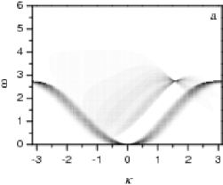
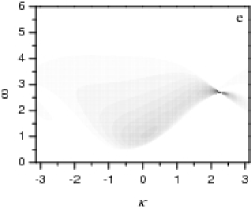
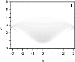
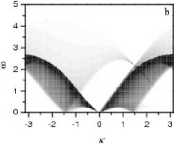
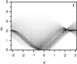
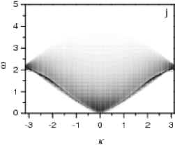
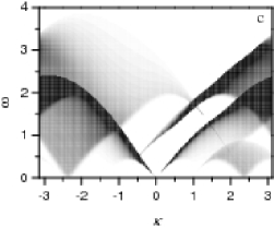
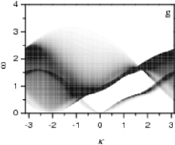
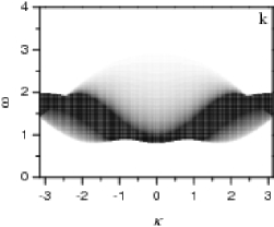
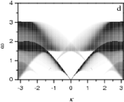
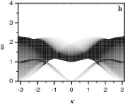
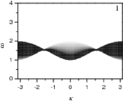
Figure 1:

Figure 2:

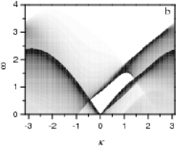
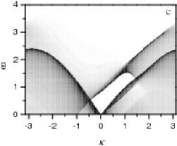
Figure 3:

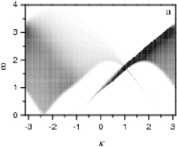
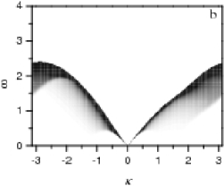
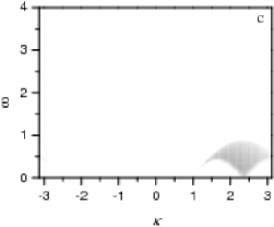
Figure 4:

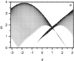
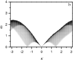
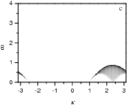
Figure 5:

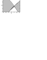
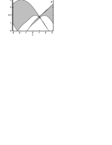
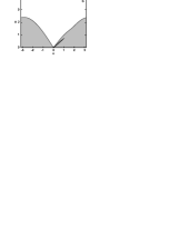
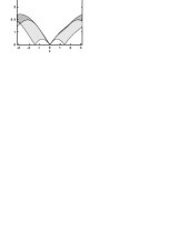
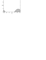
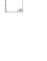
Figure 6:

Figure 7:

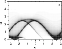
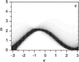
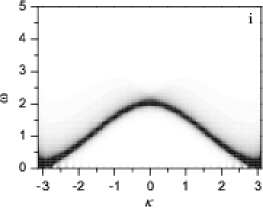
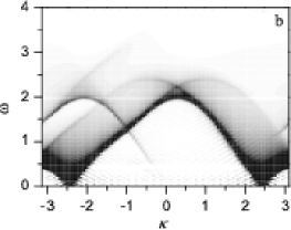
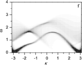
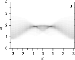
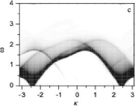
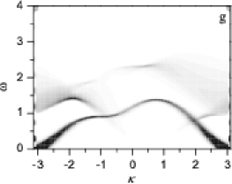
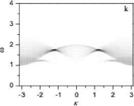
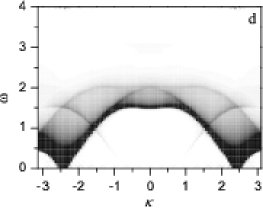
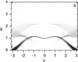
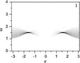
Figure 8:

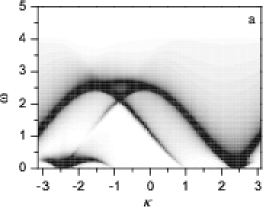
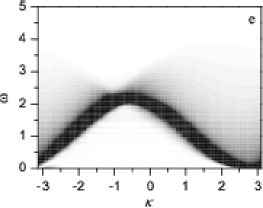
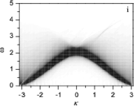
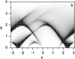
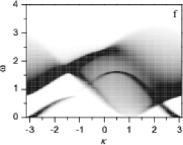
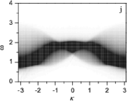
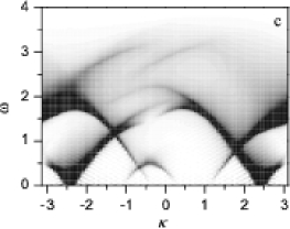
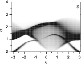
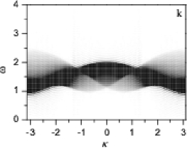
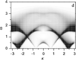
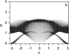
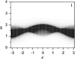
Figure 9:

Figure 10:

Figure 11:

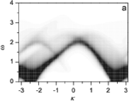
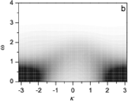
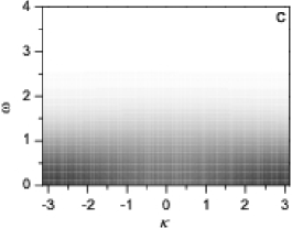
Figure 12:

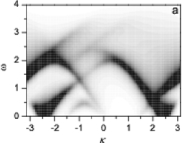
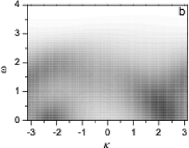
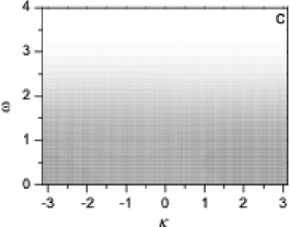
Figure 13:

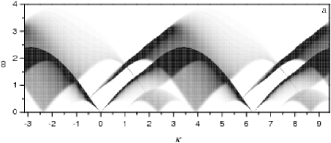
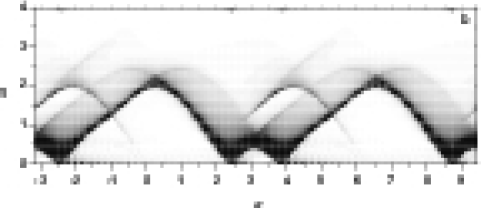
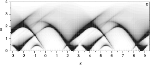
Figure 14:

References

- [1] P. Lemmens, G. Güntherodt, and C. Gros, Phys. Rep. 375, 1 (2003).
- [2] M. Oshikawa and I. Affleck, Phys. Rev. Lett. 79, 2883 (1997); I. Affleck and M. Oshikawa, Phys. Rev. B 60, 1038 (1999).
- [3] J. Z. Zhao, X. Q. Wang, T. Xiang, Z. B. Su, and L. Yu, Phys. Rev. Lett. 90, 207204 (2003).
- [4] I. Tsukada, J. Takeya, T. Masuda, and K. Uchinokura, Phys. Rev. Lett. 87, 127203 (2001).
- [5] S. Bertaina, V. A. Pashchenko, A. Stepanov, T. Masuda, and K. Uchinokura, Phys. Rev. Lett. 92, 057203 (2004).
- [6] M. Kohgi, K. Iwasa, J. - M. Mignot, B. Fak, P. Gegenwart, M. Lang, A. Ochiai, H. Aoki, and T. Suzuki, Phys. Rev. Lett. 86, 2439 (2001).
- [7] P. Fulde, B. Schmidt, and P. Thalmeier, Europhys. Lett. 31, 323 (1995).
- [8] M. Oshikawa, K. Ueda, H. Aoki, A. Ochiai, and M. Kohgi, J. Phys. Soc. Jpn. 68, 3181 (1999).
- [9] H. Shiba, K. Ueda, and O. Sakai, J. Phys. Soc. Jpn. 69, 1493 (2000).
- [10] I. Yamada and H. Onda, Phys. Rev. B 49, 1048 (1994).
- [11] J. Pommer, V. Kataev, K. - Y. Choi, P. Lemmens, A. Ionescu, Yu. Pashkevich, A. Freimuth, and G. Güntherodt, Phys. Rev. B 67, 214410 (2003).
- [12] V. A. Ivanshin, V. Yushankhai, J. Sichelschmidt, D. V. Zakharov, E. E. Kaul, and C. Geibel, Phys. Rev. B 68, 064404 (2003).
- [13] H. - A. Krug von Nidda, L. E. Svistov, M. V. Eremin, R. M. Eremina, A. Loidl, V. Kataev, A. Validov, A. Prokofiev, and W. Aßmus, Phys. Rev. B 65, 134445 (2002).
- [14] I. Yamada, M. Nishi, and J. Akimitsu, J. Phys.: Condens. Matter 8, 2625 (1996); V. N. Glazkov, A. I. Smirnov, O. A. Petrenko, D. McK Paul, A. G. Vetkin, and R. M. Eremina, J. Phys.: Condens. Matter 10, 7879 (1998); H. Nojiri, H. Ohta, S. Okubo, O. Fujita, J. Akimitsu, and M. Motokawa, J. Phys. Soc. Jpn. 68, 3417 (1999).
- [15] N. Shibata and K. Ueda, J. Phys. Soc. Jpn. 70, 3690 (2001).
- [16] T. Moriya, Phys. Rev. Lett. 4, 228 (1960); T. Moriya, Phys. Rev. 120, 91 (1960).
- [17] T. Antal, Z. Rácz, and L. Sasvári, Phys. Rev. Lett. 78, 167 (1997).
- [18] T. Antal, Z. Rácz, A. Rákos, and G. M. Schütz, Phys. Rev. E 57, 5184 (1998).
- [19] T. Antal, Z. Rácz, A. Rákos, and G. M. Schütz, Phys. Rev. E 59, 4912 (1999).
- [20] M. D. Grynberg, T. J. Newman, and R. B. Stinchcombe, Phys. Rev. E 50, 957 (1994).
- [21] D. C. Mattis and M. L. Glasser, Rev. Mod. Phys. 70, 979 (1998).
- [22] D. N. Aristov and S. V. Maleyev, Phys. Rev. B 62, R751 (2000).
- [23] M. Bocquet, F. H. L. Essler, A. M. Tsvelik, and A. O. Gogolin, Phys. Rev. B 64, 094425 (2001).
- [24] M. Kenzelmann, R. Coldea, D. A. Tennant, D. Visser, M. Hofmann, P. Smeibidl, and Z. Tylczynski, Phys. Rev. B 65, 144432 (2002); C. J. Mukherjee, R. Coldea, D. A. Tennant, M. Koza, M. Enderle, K. Habicht, P. Smeibidl, and Z. Tylczynski, J. Magn. Magn. Mater. 272-276, 920 (2004).
- [25] J. - S. Caux, F. H. L. Essler, and U. Löw, Phys. Rev. B 68, 134431 (2003).
- [26] D. V. Dmitriev and V. Ya. Krivnov, Pis’ma v ZhETF 80, 349 (2004).
- [27] J. - S. Caux and J. M. Maillet, Phys. Rev. Lett. 95, 077201 (2005); J. - S. Caux, R. Hagemans, and J. M. Maillet, J. Stat. Mech.: Theor. Exp. P09003 (2005).
- [28] V. M. Kontorovich and V. M. Tsukernik, ZhETF 52, 1446 (1967) (in Russian).
- [29] Th. J. Siskens, H. W. Capel, and K. J. F. Gaemers, Physica A 79, 259 (1975).
- [30] Th. J. Siskens and H. W. Capel, Physica A 79, 296 (1975).
- [31] J. H. H. Perk and H. W. Capel, Physica A 92, 163 (1978).
- [32] O. Derzhko and A. Moina, Ferroelectrics 153, 49 (1994); O. V. Derzhko and A. Ph. Moina, Condensed Matter Physics (L’viv) 3, 3 (1994).
- [33] A. S. T. Pires, J. Magn. Magn. Mater. 223, 304 (2001).
- [34] O. Derzhko and T. Verkholyak, Proceedings of Institute of Mathematics of NAS of Ukraine 50, 692 (2004); O. Derzhko and T. Verkholyak, Czech. J. Phys. 54, D531 (2004); O. Derzhko and T. Verkholyak, Physica B 359-361, 1403 (2005).
- [35] The difference between the one-dimensional isotropic and anisotropic models was also underlined in: J. H. H. Perk and H. W. Capel, Phys. Lett. A 58, 115 (1976).
- [36] O. Derzhko and T. Krokhmalskii, Phys. Rev. B 56, 11659 (1997); O. Derzhko and T. Krokhmalskii, physica status solidi (b) 208, 221 (1998); O. Derzhko, T. Krokhmalskii, and J. Stolze, J. Phys. A 33, 3063 (2000); O. Derzhko, T. Krokhmalskii, and J. Stolze, J. Phys. A 35, 3573 (2002).
- [37] D. Karevski, Relaxation in Quantum Spin Chains: Free Fermionic Models, in Order, Disorder and Criticality. Advanced Problems of Phase Transition Theory, edited by Yu. Holovatch (World Scientific, Singapore, 2004), pp.67-107.
- [38] J. H. Taylor and G. Müller, Physica A 130, 1 (1985).
- [39] H. Suzuura, H. Yasuhara, A. Furusaki, N. Nagaosa, and Y. Tokura, Phys. Rev. Lett. 76, 2579 (1996).
- [40] Yongmin Yu, G. Müller, and V. S. Viswanath, Phys. Rev. B 54, 9242 (1996).
- [41] O. Derzhko, T. Krokhmalskii, J. Stolze, and G. Müller, Phys. Rev. B 71, 104432 (2005); O. Derzhko, T. Krokhmalskii, J. Stolze, and G. Müller, Physica B 378-380C, 445 (2006).
- [42] O. Derzhko, T. Verkholyak, T. Krokhmalskii, and H. Büttner, Physica B 378-380C, 443 (2006).
- [43] G. Müller, H. Thomas, H. Beck, and J. C. Bonner, Phys. Rev. B 24, 1429 (1981).
- [44] I. Affleck, Field theory methods and quantum critical phenomena, in Fields, Strings and Critical Phenomena, edited by E. Brézin and J. Zinn-Justin (Elsevier, Amsterdam, 1989), pp.563-640; J. von Delft and H. Schoeller, Annalen der Physik 7, 225 (1998).
- [45] Y. Maeda and M. Oshikawa, Phys. Rev. B 67, 224424 (2003).