Prospects for Observations of Transient UV Events with the TAUVEX UV Observatory

Abstract

Transient events have posed special problems in astronomy because of the intrinsic difficulty of their detection, and a new class of observatories such as the Pan-STARRS and LSST are coming up specifically to observe these energetic events. In this paper we discuss the UV transient events from two specific sources, such as possible collisions in extrasolar planetary systems and M dwarf flares, to find the probability of their detection by space UV observatories, in particular, by the Tel Aviv University Explorer (TAUVEX). TAUVEX is an UV imaging experiment that will image large parts of the sky in the wavelength region between 1200 and 3500 Å. TAUVEX  is a collaborative effort between the Indian Institute of Astrophysics (IIA) and Tel Aviv University, and is scheduled for an early-2009 launch with at least three years of operations. The scientific instrument has been fabricated at El-Op in Israel, with the satellite interfaces, launch and flight operations provided by the Indian Space Research Organization (ISRO). The ground-based software development is the responsibility of the IIA while other aspects of the mission are the joint responsibility of IIA and Tel Aviv University. TAUVEX  Science Team (TST) have created a coherent observing program to address several key science objectives, one of them is a program to study short-scale UV transient events. We have estimated that in one year of TAUVEX observations we can expect about $90-350$ short-scale transient events. Because we obtain real-time telemetry with TAUVEX, we will be able to catch transients early in their evolution and to alert other observatories. We also present a description of TAUVEX  mission, including instrument design and its estimated performance.

Keywords TAUVEX: — space missions: planetary collisions; UV flares

1 Introduction

Astrophysical transient events include bursts, flashes, flares, gamma-ray bursts (GRBs), supernovae (SN), etc. The discovery and study of highly transient sources, especially those that rise to high brightness and then fade, has always been a major part of modern astrophysics. Historically, they were studied either as very high-energy phenomena, or in infrared (IR). For example, even before the discovery of extra-solar planets (ESPs) around main sequence (MS) stars, Stern (1994) discussed the possibility of detection of planets through IR signals from collisions with their parent stars. Recently, it was proposed that planet-planet collisions will give rise to flares, where at the flash peak time, the extreme-UV (EUV) flash can greatly outshine the host star (Zhang & Sigurdsson, 2003). On the observational side, the last two years (2006 and 2007) have been witness to the importance of the UV space survey missions in detection of UV flares (Welsh et al., 2007; Robinson et al., 2005). The conclusion derived from the Deep Lens Survey (DLS) that late-type dwarf flares constitute a dense “foreground fog" in our Galaxy, hindering any extragalactic transient search, brings back a question on a derivation of the flare frequency rate, with eventual identification of all nearby M dwarfs (Kulkarni & Rau, 2006).

With the launch of TAUVEX  on board the Indian geostationary satellite GSAT-4, the astronomical community will have access to a flexible instrument for observations in the mid-UV range of $135-400$ nm. TAUVEX  is expected to observe to a greater depth than the NASA Galaxy Explorer satellite (GALEX) Martin et. al. (2005) in $20\%$ of the sky and in three simultaneous UV bands compared to two of GALEX. The three parallel telescopes of TAUVEX  will enable to image simultaneously at three different frequency bands, thus measuring UV colours of all objects in the image frame. In parts of the orbit with little or no straylight the detection will be limited only by photon statistics, as TAUVEX  detectors are virtually noiseless (Brosch 1998a, ; Safonova & Almoznino, 2007). Effective exposure time of about 1000 sec per field in each of three TAUVEX  telescopes will yield a resultant monochromatic UV magnitude of 25, or almost 15 magnitudes better than the $TD1$ survey and with much better spatial resolution.

One of the major scientific goals of TAUVEX  is to detect and measure variability on time scales ranging from $<1\;\text{sec}-3$ years. The photometry capabilities (each detected photon is time-tagged with a precision of $\sim 128$ ms) and the possibility of repeated scans will enable the recording of UV light curves of variable sources; the time scale at which variability can be investigated will depend on the source latitude and brightness. In this article we are discussing the prospects of detecting the UV flares from active M dwarfs and possible collisions in extrasolar planetary systems by TAUVEX.

2 TAUVEX  Observatory

TAUVEX  Observatory is an array of three identical, 20 cm aperture, co-aligned F/8 Ritchey-Crétien telescopes mounted on a single bezel and enclosed in a common envelope. Each telescope consists of a primary mirror, a secondary mirror and 2 doublets of field-correcting lenses that maintain a relatively constant focal plane scale across the nominal field of view of $0.9^{\circ}$ and serve as Ly-$\alpha$ blockers when heated to $25^{\circ}$ C. The primary and secondary mirrors are both lightweighted zerodur coated with Al + MgF₂ with an effective reflectivity of better than 90%. There are four filters per telescope offering a total of five different UV bands for observation (Fig. 1).

The detectors are photon-counting imaging devices, made of a CsTe photocathode deposited on the inner surface of the entrance window, a stack of three multi-channel plates (MCP), and a multi-electrode anode of the wedge-and-strip (WSZ) type. Properties of the instrument are summarized in Table 1.

Table 2 contains pre-launch predictions for the in-orbit performance of TAUVEX  ​​. The nominal mode of operation of TAUVEX  is to scan along a single line of celestial latitude, with entire sky coverage attained by rotating the mounting deck platform (MDP). Exposure time in a single scan is limited to 216 seconds at the celestial equator, but increases with declination to a theoretical maximum of $\sim 86,400$ seconds per day at celestial poles (see Table 2).

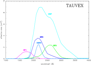
Figure 1: The spectral range of the TAUVEX  filters; effective areas at the beginning of the mission versus wavelength.

Table 1: Instrument Parameters.

Mirrors (2 per telescope)	:	hyperbolic, zerodur substrate, Al+MgF2 coating
Optics	:	F/8 Ritchey-Chrétian; 2 doublet CaF2 lenses
Diameter	:	20 cm aperture
Detector	:	3-stack MCP with 25 mm CsTe photocathode
	:	and Wedge-and-Strip anode
Observational mode	:	Scanning
Total payload weight	:	69.5 Kg
Locations of the filters
Telescope:		Filters:
T1	:	SF1; SF2; BBF
T2	:	SF2; SF3; BBF
T3	:	SF1; SF3; NBF3

Table 2: Predicted Performance

Wavelength coverage	: $1250-3500$ Å
Field of View (FOV)	: $0.9^{\circ}$
Angular resolution	: $\sim 10^{\prime\prime}$
Expected source position localization	: $\sim 5^{\prime\prime}$ (for a $15^{m}$ object)
Time resolution	: 128 milliseconds
Minimal exposure time∗	: 216 seconds
Filters central wavelengths and bandpasses
Filter:	Wavelength (Å)	Width (Å)
NBF3	:      2200	:      200
SF1	:      1750	:      500
SF2	:      2200	:      400
SF3	:      2600	:      500
BBF	:      2300	:      1000
Point source sensitivity (200 s)	:      (For an O type star)
BBF	:           $V\approx 22.2$
SF3	:           $V\approx 20.2$
SF2	:           $V\approx 20.8$
SF1	:           $V\approx 20.3$
NBF3	:           $V\approx 19.2$
Bright limit (point source, BBF)	:  $F_{\lambda}=1.3\times 10^{-11}$ erg cm-2 s-1 Å-1

*this exposure time is for $\delta=0^{\circ}$ for a source at the centre of FOV; it increases with declination and reaches theoretically $\sim 86000$ seconds on the Poles.

The primary data product of TAUVEX  pipeline is a calibrated photon list where each photon is tagged by sky position and time, after correction of all instrumental effects. Tools will be provided to extract multi-band images of the sky from these photon lists. We will also create special tools intended for analysis of variable sources. The first of these is a real-time tool in which the brightness of any point source in the field will be checked for variability both between frames, that is, within an observation, and by comparison with predicted count rates from historical observations. If a significant event, over and beyond normal noise, is found, a responsible scientist will be immediately notified and follow-up observations may be scheduled with other ground and space based telescopes, such as, for example, Indian Astronomical Observatory (IAO) at Hanle. The other tool will run as part of the normal pipeline, perhaps days after the observation. This will produce a time history of every source found during normal observations, which can then later be examined for variability.

2.1 TAUVEX  Team Science Investigations

As an observatory class mission, TAUVEX  has a broad scientific program. TAUVEX  is different from most missions in that it is only a scanning instrument; pointed observations are not possible. Despite this major disadvantage, the location of TAUVEX  in geostationary orbit allows for exceptionally deep observations of areas near the poles with very low backgrounds. Thus, one of the major scientific programs of TAUVEX  is the Deep Exposure Polar Survey (DEPS), in which $\sim 1400$ square degrees around each Celestial Pole is intended to be covered with a uniform accumulated exposure of 5000 sec in the first year of operation, followed by a repeat of another 5000 sec in the second year. This is expected to achieve a depth of $25^{m}$ in three UV bands. (All magnitudes are quoted as per the monochromatic scale of Hayes & Latham monochromatic (1975).) Another major survey is the Galactic Plane Survey (GAPS), which will also be performed during the first two years of operations and will cover $\sim 1500$ square degrees with an average accumulated exposure of 1000 sec. It is expected that in total 5-7 years of TAUVEX  lifetime the whole sky will be covered. Most of the surveys will be performed in three TAUVEX  principal filters, SF1, SF2 and SF3, which span the spectral region from somewhat longer than Lyman $\alpha$ to 320 nm with three well-defined bands. Three filters define two colour indices in the UV, and the combination of these measurements with data from the optical and infrared allows the derivation of even more colour indices.

3 UV Emission from Celestial Collisions

The phenomena of one celestial body colliding with another is quite common on all astronomical scales, from asteroids bombarding planets to recently discovered collisions of massive galaxy clusters Clowe et al. (2006); Jee et al. (2007). The origin of blue stragglers in the globular clusters is due to merging of two, or even three, MS stars of $\sim 0.8$ $M_{\odot}$. Perhaps, half the stars in the central regions of some globulars have undergone one or two collisions over a period of $10^{10}$ years (Zwart et al., 1999). White dwarf (WD) binaries with periods $<5$ mins will merge in a few thousand years, and neutron star–white dwarf (NS–WD) binaries with periods of $\sim 10$ mins have been observed (Tamm & Spruit, 2001).

Over the past few decades, a standard model for planetary system formation has emerged, in which the final stage is now strongly associated with a significant number of giant impacts on each of the young forming planets Stern (1994). Giant Impact Models (GIM) are often invoked for explaining the formation of planetary systems, the Mars-sized terrestrial impactor believed to be responsible for the formation of the Moon was such an impact Stevenson (1987). However, even at later stages of planetary system life, such giant collisions are possible. In the past decade about 200 ESPs have been detected and they are a rapidly growing sample. Most of these ESPs are giant ‘Hot Jupiters’, locked in very short-period orbits with their star. It is reasonable to expect planetary and stellar-planetary collisions in such systems.

Collisions on all scales can be very energetic. A recent example in our own Solar System is that of the comet Shoemaker-Levy which collided with Jupiter. If a WD smashes into a MS star like our Sun with an incoming velocity of, say, $\geq 700$ km/sec, the massive shock wave would compress and heat the Sun, the nuclear reactions will speed up, and, in about an hour, the Sun would release a thermonuclear energy of about $10^{49}$ ergs, and the resulting instabilities would blow the Sun apart in few hours (Sivaram, 2007). This equivalent of a nuclear explosion of a star was recently revoked in a slightly different context by Brassart and Luminet (2008) for the case of a star getting too close (or colliding) to a supermassive black hole whose tidal forces would create stresses inside the star that may trigger a nuclear explosion and give out a burst of an electromagnetic radiation. Gamma-ray bursts (GRBs) once were thought to be of a Galactic origin; one popular model being of an asteroid-size objects (with $\sim 10^{32}$ gm of mass) impacting a neutron star (NS). In such case, with the impact velocity at a surface of a NS of $\sim 0.1\,c$, the released kinetic energy would be $\sim 10^{52}$ ergs (or $T\sim 10^{9}$ K), with most of the radiation in the form of a few hundred Kev $\gamma$-rays. Recently, the impact theory was revived by proposing an alternative model for the short-duration GRBs, explaining them as supernovae followed the collision of compact objects (Sivaram, 2007).

3.1 Planet-planet collisions

Stern (1994) has estimated that for planetary impacts with total collisional energy above $5\times 10^{34}$ ergs the dominant heat sink would be radiation to space. We will consider here a Jovian planet (with mass $\sim M_{\rm J}$) being hit by a terrestrial-size planet (with mass $\sim m_{\rm E}$), as in such a case the total impact energy is of the order $E_{\rm imp}\sim GM_{\rm J}m_{\rm E}/R_{\rm J}\sim 10^{40}$ ergs. Giant impacts range from glancing events to direct head-on collisions. It is reasonable to assume hyper-velocity impacts, as, for example, in the end-member archetypes of planetary collisions. However, even the proposed origin of the Moon requires an impact velocity just barely above the two-body escape velocity (Asphaug et al., 2006). Still, even if a giant impactor approaches the target with negligible velocity, its decent into the target’s gravitational  potential well will cause it to impact at near escape velocity. Therefore, in our calculations we assume the starting impact velocity as two-body mutual escape velocity, which for terrestrial and Jovian-like bodies will be

$$v^{2}_{\rm imp}\approx v_{\infty}^{2}+v_{\rm esc}^{2}\,,$$ (1)

where $v_{\infty}$ is the random velocity of the encountering bodies. Assuming $v_{\infty}=0$, we obtain

$$v_{\rm esc}=\sqrt{\frac{2G(M_{\rm J}+m_{\rm E})}{(R_{\rm J}+r_{\rm E})}}\approx 40\,\text{km/sec}\,.$$ (2)

The friction between the impactor and the atmosphere of the impacted planet, which increases in density as the target descends, generates an intense shock wave, heating the target. It was assumed in Zhang & Sigurdsson (2003) that since the energy deposit during the impactor descent is much greater than the corresponding Eddington luminosity of the target, $L^{\rm J}_{\rm Edd}$, the peak luminosity resulting from the hot spot created by the impactor will be $L_{\rm pk}\sim\eta L^{\rm J}_{\rm Edd}\approx L^{\rm J}_{\rm Edd}$. This luminosity will be produced by the hot spot with a peak temperature of $\sim 10^{5}$ K and in a time-scale of few seconds, giving rise to an electromagnetic flash at far-UV $\lambda\sim 450$ Å. However, it is quite likely that $\eta$, the factor correcting for radiative inefficiencies in Zhang & Sigurdsson (2003), is not unity. Besides, the gas opacity of the atmosphere is crucial for the escape of radiation from the shocked matter, which was not considered in Zhang & Sigurdsson (2003).

Let us assume the atmospheric entry at velocity $v$ and angle $\phi$ (see Fig. 5 in Appendix A). The force of drag on an impactor is $F_{\rm D}=1/2C_{\rm D}\rho_{a}Av^{2}$, where $\rho_{a}$ is the atmospheric density and $C_{\rm D}$ is the coefficient of atmospheric drag ($C_{\rm D}$ ranges from $1/2$ for spheres to $\approx 1/7$ (Chyba et al., 1993) for cylinders). The power released due to the drag will be

$$\dot{E}=\frac{1}{2}C_{\rm D}\rho_{a}Av^{3}\,,$$ (3)

where $A$ is the front area of the impactor. If we assume that all dissipated energy is lost as radiation, $\eta\rho_{a}Av^{3}\sim\sigma AT_{\rm R}^{4}$, we obtain

$$T_{\rm R}\sim\left(\frac{\eta\rho_{a}v^{3}}{\sigma}\right)^{1/4}\,,$$ (4)

where $\sigma$ is the Stephan-Boltzmann constant and $\eta$ is a fraction of energy going into heat. We assume $\eta\approx 1$ ($T_{\rm R}$ it is relatively insensitive to it). The temperature estimates for different impact velocities, taken in the range $10-40\,\text{km/s}$, are given in Table 3. We see from the table that $T_{\rm R}$ strongly depends on the velocity of the impactor and a wide range of temperatures is possible.

Table 3: This table presents estimates of $T_{\rm R}(K)$ from Eq. 4 as a function of density $\rho$ (g/cm³) and impact velocity $v$.

$\rho\setminus v$	10 km/sec	40 km/sec
$10^{-8}$	$\sim 3,600$	$\sim 10,000$
$10^{-6}$	$\sim 11,500$	$\sim 32,500$
$10^{-4}$	$\sim 36,000$	$\sim 100,000$
$10^{-3}$	$\sim 65,000$	$\sim 180,000$

For a thermal spectrum, a region of $2-6\times 10^{4}$ K represents the near-UV part of the spectrum. With $T_{\rm R}\sim 10^{5}$, the predominant radiation will be in the far-UV region, however, the prompt radiation, firstly, strongly depends on initial velocity, and, secondly, as was shown in detail in Chevalier & Sarazin (1994), since the gas is optically thin in the top layers of atmosphere, the initial radiation will be concentrated in the form of emission lines. At $\rho\approx 10^{-6}$, merely a $\sim$ second after the start of a descent, the shocked atmosphere is optically thick, shock becomes a source of black-body continuum radiation, and the favoured emission is in $1000-3000$ Å  initially. This radiation can escape in the prompt phase from the vicinity of the shock front, but radiation bluer than $\sim 900$ Å  is trapped very close to the shock and is absorbed in a narrow pre-shock region (thus only the longer wavelength UV radiation can escape). At this prompt phase, the luminosity can reach $L_{\rm UV}\sim 10^{31}$ erg/sec, and the total integrated energy released during descent may reach $\sim 10^{32}$ ergs (see calculations App. A). The flux of UV photons from the Sun at the Earth (at 1 A.U.) is $\sim 3\times 10^{14}$ phot/cm² s, from a distance of 10 pc it would be $\sim 50$ phot/cm² s. The flare flux at Earth in the UV at this distance would be $\sim 10^{3}$ phot/cm² s, thus outshining any MS host star later than B5. The maximum expected flux at Earth is in a range:

	at 10 pc	at 1Kpc
Host star	$1-50$ ph/cm2 s	$10^{-2}-10^{-3}$ ph/cm2 s
(G, K)
Coll. event	upto $10^{3}$ ph/cm2 s	upto $1$ ph/cm2 s
at 3000 Å

The radiation in the prompt phase of the collision can be defined as a flare–a sudden, rapid and intense variation in brightness. Flares are a one-time event. The flares from the collisions will be followed by repeated flashes that can be produced through two different mechanisms. One type of flash is caused by the target planet’s rotation. Since the typical spin period of giant planets is $\tau_{2}<1$ day, one expects a periodic luminosity modulation of the UV light curve, caused by an expanding hot spot entering and leaving the line of sight over a time-scale of $\tau_{2}$. This may also be detectable in optical bands.

The second type of flash is caused by a fall-back of material in the case of the impactor reaching the surface of the target. Prompt flare radiation pressure would drive a fraction of the impacted material outwards; as the radiation pressure drops, the material will fall back on the surface at $\sim v_{\rm esc}/2$. This fall-back can lead to reheating and repeated flash(es) of decreasing brightness. If we consider a universal hydrodynamic scaling relation, the distance traveled in time $t$ is

$$R=\left(\frac{1}{\alpha_{s}}\frac{E}{\rho_{a}}\right)^{1/5}t^{2/5}\,,$$ (5)

where $\alpha_{s}$ is $1.3-1.7$ for a spherical blast wave. The free-fall time would be of order of $\tau_{3}\sim$ few hours. The first flash will have the energy of $\sim 1/4$ of the flare.

Thus, we establish three important time-scales,

$\tau_{1}$	flare	upto $10^{3}$ s
$\tau_{2}$	modulation due to spin	$\lesssim 1$ day
$\tau_{3}$	flashes due to fall-back	$\sim$ few hours

More exotic cases of planetary collisions are possible. The discovery of several “very hot Jupiters" (Hébrard et al., 2004) brings an interesting possibility that because of their proximity to the host star, they may have their atmospheres evaporated; they are the new class of planets called “chthonians". In this case, the direct impact onto a hot chthonian surface will produce a flare with a temperature $T\approx 1500-2000$ K, with consequent flashes of decreasing brightness.

If two ‘Hot Jupiters’, tidally locked with the host star, collide, such collision could generate $\sim 10^{45}$ ergs with peak temperature at $\sim 2\times 10^{5}$. For an event duration of 10 hours, we can expect an EUV fluence of $10^{5}$ phot/cm² from a collision at 10 Kpc, while the fluence from the host star will constitute most probably only $\sim$1 phot/cm². For the TAUVEX  sensitivity range this will correspond to about $10^{4}$ phot/cm². If the rotation period is about one day, this flux will be modulated over a day.

3.2 Stellar-planetary collisions

Many extra-solar Jovian planets are in very tight orbits around the star. Out of the total of 246 extra-solar planetary systems discovered to date, there are, at least, 30 planets with orbits less than 1 A.U. from the host star. Assuming the velocities are of order $\sim 200-300$ km/sec, the planet can spiral down in $\sim 10^{8}-10^{9}$ years (due to the gravitational radiation). It is conceivable that a collision between the planet and the star might be frequent, where the collisional time-scale will be of the order $10^{6}$ sec. For the impact velocity of $\sim 600$ km/sec, the kinetic energy release in the collision will be $\sim 10^{46}$ ergs with a peak temperature, following Eqs. (3) and (4), of $T_{\rm peak}\sim 6\times 10^{5}$ K. This would imply the soft X-ray flux of $\sim 10^{4}$ ergs/cm²/sec at a distance of 10 pc. The flux at Earth from the distance of 10 Kpc is $\sim 10^{-6}$ ergs/cm²/sec. This soft X-ray flash can last a few hours and is $10^{8}$ times more intense than the strongest solar flare. The initial soft X-ray flash will be followed by intense EUV-UV radiation for few days, with flux at Earth of the order $\sim 0.3$ ergs/cm²/sec at 10 pc distance. From 10 Kpc, the UV flux will be $\sim 3\times 10^{-7}$ ergs/cm²/sec. In the TAUVEX  bands we can expect $\sim 10^{8}$ phot/cm² sec from a distance of 10 pc and $10^{2}$ phot/cm² sec from a distance of 10 Kpc. We illustrate these values in Table 4.

Table 4: Expected flux at Earth in different bands

Distance	X-ray	EUV	TAUVEX
10 pc	$80-100$ ergs/cm2 s	$0.3$ ergs/cm2 s	$10^{8}$ phot/cm2 s
10 Kpc	$\sim 10^{-5}$ ergs/cm2 s	$3\times 10^{-7}$ ergs/cm2 s	$10^{2}$ phot/cm2 s

Impacts of comets with young stars having dust debris disks are also energetic collision events. In such case, however, the diffuse structure of a comet with its extensive coma would reduce the intensity of the power, or flux, of the flare that may result from a collision. The volatile elements would vaporise, or sublimate, on approaching the star (a comet could even completely disintegrate). Use of the equations in the Apendix A shows that the dependence on the area (and mass) would give a significantly lower temperature (and total released energy) than in the case of an impact of a larger planetary body. Most of the radiation would be in the infrared or longer optical wavelengths. (For example, collision of a Shoemaker-Levy comet with Jupiter resulted in intense IR radiation.) There could be also an initial optical flash, but the UV flux would be substantially smaller.

4 M-dwarf flares

Another type of short-scale transients are stellar flares from late-type stars, for example, M dwarfs. M dwarfs account for more than 75% of the stellar population in the solar neighbourhood (up to 1 Kpc). These stars are known to possess strong magnetic fields with high coronal activity and associated UV line emission (Mitra-Kraev et al., 2005) and a vast majority of UV short transients is associated with a single physical type of astrophysical source, that is, stellar flare eruptions on K and M stars. These flares exceed the quiescent phase luminosity by two or three orders of magnitude and are a thousand times more energetic than solar flares. The peak temperature (in the active or disturbed regions) of the flare reaches $10^{4}-3\times 10^{4}$ K, which implies an UV peak, at luminosities of $10^{25}-10^{26}$ W. For such a flare on, for example, Proxima Cen, this could correspond to a flux at Earth of $10^{5}-10^{6}$ UV phots/cm² for a period of several hours. The M dwarf flare 100 pc away will produce UV flux at Earth of $10-10^{2}$ phots/cm², which is detectable by TAUVEX. Studying the frequency of dMe flares can be important from several standpoints.

• The level of chromospheric activity may vary with dMe stellar age and mass (Gizis et al., 2002). Observations (see Welsh et al. (2007) and references within) indicate that activity strength (as measured by the ratio of H$\alpha$ luminosity to the stellar bolometric luminosity) increases with the spectral class—earlier dMes have higher flare energies. However, as was discussed in Kulkarni & Rau (2006), there may be a fraction of late-type dwarfs that retain their activity for a longer period or may have had activity induced later in their lives.

• A derivation of the UV flare frequency rate on M dwarfs is also important for the study of habitability zones on possible associated ESP systems (Turnbull & Tarter, 2003).

• Lastly, the estimated dMe transients annual rate (Kulkarni & Rau, 2006) of $R_{R}\sim 10^{8}\,\text{yr}^{-1}$ implies the existence of immense fog of M dwarfs that hinders any extragalactic transient search—the foreground fog of dMe flares ensures that the false positives outnumber genuine extragalactic events by at least two orders of magnitude. The clear identification of all suspect dwarfs, especially over the extragalactic fields, will ensure that the extragalactic surveys, like, for ex. PANSTARRS or LSST, will not drown in false detections.

The recent detection of a flare star by GALEX (Robinson et al., 2005) has shown the power of UV observations in such studies. The peak of the radiation is at $\lambda<4000$ Å (van den Oord et al., 1996) and optical photometry will only sample a wing of this distribution against the bright stellar photosphere. By contrast, the continuum and line emission during a flare in the UV will cause a much greater spike in the intensity, by a factor of 1000 or more, which will be seen against a much fainter stellar photospheric background.

5 Prospects of Observations with TAUVEX

5.1 Estimates of frequency and detectability of planetary collisions

A large number of collisions should be happening in dynamically young systems (like planetary systems in formation), but there could be collisions in mature systems as well. For example, $\tau$ Ceti has more than 10 times the amount of dust as the Sun. Any planet around $\tau$ Ceti would suffer from large impact events roughly 10 times more frequently than Earth. Even more interesting is $\epsilon$ Eri, which has $\sim 10^{3}$ more dust than is present in the inner system around our Sun. It has a detected planetary system as well; with one $1.55M_{\rm J}$ mass planet at $3.4$ A.U. At, say, 3000 Å, the flux from $\tau$ Ceti at Earth is $3.4\times 10^{-11}$ ergs/cm² sec, which is equivalent to $\sim 6$ phots/cm² sec. The UV flare in its system may produce up to $\sim 4\times 10^{-8}$ ergs/cm²sec, or up to $\sim 6\times 10^{3}$ phots/cm²sec in the UV. The flux contrast is dramatic. Most known exoplanets orbit stars which are roughly similar to our own Sun, that is, MS stars of spectral categories F, G, or K, with the current count (year 2007) of ESP candidate systems of 252, most of them within 1 Kpc distance from the Sun.

The flux at Earth from a self-luminous thermally dominated object is

$$F_{\lambda}=\left(\frac{R}{D}\right)^{2}\int_{\lambda_{1}}^{\lambda_{2}}B_{\lambda}(T)d\lambda\,,$$ (6)

where $D$ is the distance to Earth, $R$ is the radius of the source, $B_{\lambda}(T)$ is the Planck function, and the integration limit refers to the width of a given bandpass. Fig. 2 depicts the UV flares flux curves from a terrestrial-size hot spot with $T=20000$ K as seen at different distances from Earth. It also shows the black body flux curves for a solar type (G8V, $\tau$ Ceti taken as an example) star, a cooler star (K2V, $\epsilon$ Eri as an example) as seen from the same distances, along with UV sensitivity of TAUVEX  in all filters for 1 Ksec exposure. For comparison, Fig. 3 shows UV sensitivity of TAUVEX in all filters (and filters wavelength coverage) for different exposure times. It is clearly seen that for an average exposure of 1000 sec the flares are easily detectable by TAUVEX  ​​, even if they occur at 1 Kpc distance. These calculations demonstrate that hot spots resulting from the terrestrial-size object impacting the giant planet are sufficiently bright to be detected from a flux sensitivity standpoint.

Figure 2: Thermal flux curves for G8V and K2V stars and UV collision flare ($2\times 10^{4}$ K) as seen at different distances from Earth. Also shown are the sensitivity limits for a 5 $\sigma$ detection by TAUVEX  in all filter bands for 1000 sec exposure (the span of each line shows the wavelength coverage of that filter). This shows a clear detectability of the flares from collisions in the situation of an average non-negligible sky background.

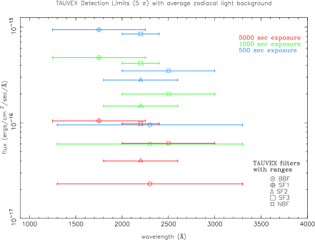
Figure 3: Sensitivity limits for a 5 $\sigma$ detection in all filter bands for proposed TAUVEX  surveys. The span of each line shows the wavelength range of that filter.

In young planetary systems the central star is surrounded by planetesimals with a few embryos of mass $10-100M_{\oplus}$. We can easily assume existence of $10^{8}-10^{9}$ planetesimals in $\sim 100$ km diameter, or more! In a $(1\text{A.U.})^{3}$ volume the number is $n=10^{-32}$ cm^-3. The mean time between the collisions is of order $t_{c}\sim 1/(n\sigma v)$. With $v=10^{2}$ km/sec, $\sigma\sim(GM/v^{2})^{2}\sim 10^{16}-10^{7}$ cm², and time $\sim 10^{6}$ sec, we can have 10 colls/year (of $\sim 10^{2}$ km size objects) in a typical system. If there are $10^{7}-10^{8}$ such systems in a whole Galaxy, we can expect $10^{8}-10^{9}$ such events per year.

Using the annual rate of events, the detection rate can be found. Let $\tau$ be the exposure time per FOV (say, $1000$ sec). The number of flares per exposure is

$$N_{f}=\frac{R_{f}\,\tau\Delta\Omega}{4\pi}\,,$$ (7)

where $\Delta\Omega\approx 2\times 10^{-4}$ sr is the TAUVEX  FOV, and $R_{f}\sim 10^{8}$ yr^-1 is an annual rate, estimated above. In one year of observations we can expect about $90-350$ such events. We can differentiate these flares from other transients (like, for instance, flares from M dwarfs, discussed in the next section) because of the temporal modulation due to the planet’s rotation, or even the orbital period, if it is a hot Jupiter. Occurence of repeated flashes (flares) of diminishing intensity due to the infall (and subsequent rebound) of debris falling back on the impactor is an additional clue. Every such collision will be followed by a long-duration infra-red emission, which could perhaps be detected on the ground as a follow-up.

5.2 M-dwarf flares

During TAUVEX surveys, a simultaneous monitoring of a $\sim 1^{\circ}$ field of view in three UV bands will allow the accurate determination of UV fluxes and colours at high time resolution ($\sim 0.1$ sec) of any detected flare. Three UV bands mean two UV colours, and obtaining flare colours allows estimates of temperatures and sizes of active regions. For example, in assumption of the black body emission (which is only one of several possible flare model scenarios, but still being widely used in the studies of flares, see Robinson et al. (2005) and references within), we can determine the relation between the black body and the measured SF1/SF2 and SF2/SF3 flux ratios. This is calculated by convolving the black body spectrum for different temperatures with the effective area curves for three TAUVEX principal survey filters, SF1, SF2 and SF3, and then normalizing to the total effective area of each filter. This gives the expected flux for a black body in each filter, which can later be directly related to the average flux determined from the measured count rates. The relation between temperature and flux ratios is shown in Fig. 4.

Figure 4: Relation between black body temperature and the SF1/SF2 and SF2/SF3 flux ratios, determined by convolving the appropriate blackbody distribution with TAUVEX principal survey filters (SF1,SF2,SF3) effective area curves.

The comparison of measured flux ratios of observed flares with the theoretical will give an estimate of the effective temperature and a black body of a given temperature has a well-defined emission. Having determined the temperature, we can define the effective stellar surface coverage required to produce the observed flux at Earth, assuming (or determining) the distance to the star. As a result, we can then determine the total energy of the flare by integrating over the approriate black body curve.

We can estimate the flares detection rate in the TAUVEX  surveys. If we take the exposure time per FOV as $\sim 5000$ sec in DEPS and $\sim 600$ sec in GAPS, the number of flares per exposure is (see Eq. 7)

$$N_{F}=\frac{R_{F}\,\tau\Delta\Omega}{4\pi}\,,$$ (8)

where $R_{F}\sim 10^{8}$ yr^-1 is an annual all-sky rate of fast transients in B band, estimated elsewhere (Becker et al., 2004; Kulkarni & Rau, 2006). Then $N_{F}^{DEPS}=0.25$ and $N_{F}^{GAPS}=0.03$. Assuming 20% efficiency in utilizing time in DEPS and 30% in GAPS, we can estimate that in a year of observation we will observe $N^{DEPS}_{F}\sim 950$ and $N^{GAPS}_{F}\sim 290$.

Identification of any dMe flare in DEPS (with its high ecliptic latitude) may help extragalactic surveys, such as, for example, DLS, or even, GRB searches, as some of dMe flares were already mistaken for GRBs (Kulkarni & Rau, 2006). The two colours obtained by TAUVEX  may be used to discriminate against genuine extragalactic transients—the Rayleigh-Jeans tail of a blackbody, for example, has a distinctly different spectrum ($f_{\nu}\propto\nu^{2}$) than, say, synchrotron radiation ($f_{\nu}\propto\nu^{\alpha}$, with $\alpha\sim-1$).

6 Conclusion

In this paper we considered two sources of the UV short-scale transient events, namely, the UV flares from the active late-type stars and from possible collisions in extrasolar planetary systems. UV transients can be broadly divided into three categories: ‘regular’, ‘expected’ and ‘unexpected’ events. ‘Regular’ events would include CVs, recurring novae, etc. These observations are part of a regular TAUVEX observational plan; they will be scheduled according to the submitted proposals. The scientific output of these is the responsibility of the respective scientists who submit the proposal. ‘Unexpected’ events include SNs, GRBs, UV/X-ray flares resulting from the tidal disruption of a star passing too close to a supermassive black hole (the latter event can result in a series of UV/X-ray flares, initially from a star being blown apart by an internal nuclear explosion (Brassart & Luminet, 2008), subsequently from the stellar debris falling back into the black hole (Gezari et al., 2008), and finally from the debris stream collision with itself long after the disruption (Kim et al., 1999)). These transients are impossible to predict, they are of a long duration (from days to years), and some, for example, SNd Ia and GRBs are intrinsically faint in the UV.

The category of the ‘expected’ UV transients, that would include the flares from the late-type stars, both known and unknown, and UV flashes from the collisions in the extrasolar planetary systems, is however the one that is the subject of the present investigation. The latter can include the planet-planet collisions, planet-star collisions and smaller objects/debris collisions (comets, asteroids, etc.). We have concentrated on the first two types of collisions as these would produce the strong signal in the appropriate energy range, detectable by TAUVEX. We discussed the dynamics of planetary collisions in some detail, especially the collisions of terrestrial-mass planets with Jovian planets and hot Jupiters. Dynamics of atmospheric drag, shock-wave bounce, infall of debris, etc. are taken into account. The duration of the events as well the UV fluence expected from events at 10 pc and 10 Kpc are estimated. The flux from the UV flare event in contrast to emission from the host star is estimated. Expected annual rate of such events is calculated for the FOV of TAUVEX  detector.

TAUVEX  observatory will monitor large areas of the sky with different cadences and is well suited for variability studies on scales ranging from less than a second to months. We will implement programs to monitor TAUVEX  data in real-time and to notify the responsible scientist in the case of a flare. Follow-up observations with ground-based telescopes will be immediately initiated.

The next step in our preparations for TAUVEX  observations is going to be the simulation of the late-type star flare spectrum through available software (for example, the CHIANTI package) over the TAUVEX  wavelength range. This range contains many emission lines together with the continuum radiation. Assessing the relative contributions from continuum and/or emission lines at near UV wavelengths is still an open problem for flare research (see Robinson et al. (2005) and discussion therein). Convolution of the simulated spectrum with TAUVEX  filters response functions will give us the emission lines contained within the filters. We will derive a set of templates of TAUVEX  filters ratios for different values of electon pressures and different differential emission measures (DEM). Thus, if a flare is observed by TAUVEX  ​​, the comparison of the theoretical flux ratios with the measured ones can help in determining the value of the plasma electron density during the flare event, in the assumption that the increase in electron pressure during the flare has a major influence on the ratios (Welsh et al., 2006). In addition, since GALEX has produced a catalog of GALEX transient events (Welsh et al., 2005), the predictions for the stellar-planetary collision UV flashes could be tested against the existing GALEX data set, and this topic will also be addressed in the forthcoming paper.

7 Additional Information

The most extensive description of proposed TAUVEX science, predicted performance and planned calibrations till date is presented in the special issue of the Bulletin of Indian Astronomical Society BASI June (2007).

Proposed TAUVEX  launch date is January-February 2009. This date can be revised but the launch is scheduled to be no later than April 2009. The latest updates on the launch date and technical information about the initial performance results and information about observing with TAUVEX  can be found in the TAUVEX Observer’s Manual (Safonova & Almoznino, 2007) and on the TAUVEX web site at: http://tauvex.iiap.res.in. Guest Investigator questions can be directed to TAUVEX  help desk at tauvex@iiap.res.in, or to Dr. M. Safonova at rita@iiap.res.in.

8 Acknowledgments

It is a pleasure to thank many dedicated people who are working hard to make TAUVEX  mission happen, most of all, the TAUVEX  Core Group, the GSAT-4 group at the ISRO Satellite Centre (ISAC) and the engineers at El-Op. We also thank the anonymous referee for exremely helpful and useful comments, and especially for attracting our attention to a case of stellar disruptions by supermassive black holes, which is now included in one of the TAUVEX Key Areas observational plan.

Appendix A Appendix. Detailed Calculations for Planetary Collisions

Figure 5: Atmospheric entry at an angle $\phi$, $90^{\circ}$ is grazing, $0^{\circ}$ is head-on.

The above figure depicts the atmospheric entry of a body mass $m$ at an angle $\phi$ with initial velocity $v_{i}$ into the atmosphere of a larger body. Here $z$–height of the atmosphere, $r_{\rm p}$ is the radius of a target, $r$–radial coordinate. The most general equation of motion for the descent is

$$\frac{v}{\cos{\phi}}\frac{d\phi}{dt}=g-\frac{v^{2}}{r}-\frac{C_{\rm D}A}{m_{\rm E}}\frac{\rho_{a}}{2}\frac{v^{2}}{\cos{\phi}}\,,$$ (A1)

where $\rho_{a}$ is atmospheric density, $A$ is interacting area of the impactor, $g$ is acceleration due to gravity and $C_{\rm D}$ is the coefficient of atmospheric drag. Assuming isothermal atmosphere, $\rho(z)=\rho_{0}\mathrm{e}^{-\mu z}$ with $1/\mu=R_{g}T/M_{g}$ the scale height, where $R_{g}$ is the gas constant, $M_{g}$ is the molecular weight of the atmosphere and $T$–the temperature. After introducing the dimensionless Chapman parameters

$$\bar{v}=\frac{v\cos{\phi}}{v_{i}}\quad\text{and}\quad Ch=\frac{\rho_{0}}{2\mu}\frac{C_{\rm D}A}{m}\sqrt{\mu r}\mathrm{e}^{-\mu z}\,,$$ (A2)

the equation becomes

$$\bar{v}^{2}+\left(Ch\right)^{\prime\prime}+\bar{v}\left(Ch\right)^{\prime}=\frac{1-\bar{v}^{2}}{v\bar{v}^{2}Ch}\cos^{4}{\phi}-\sqrt{\mu r}\frac{L}{D}\cos^{3}{\phi}\,,$$ (A3)

where $L/D\sim 1$ is the lift-to-drag ratio. The deceleration will be

$$\frac{d\bar{v}}{dt}=-\sqrt{g\mu}\bar{v}^{2}\frac{Ch}{\cos{\phi}}\,.$$ (A4)

The time of flight is

$$t_{2}-t_{1}=\frac{1}{\sqrt{g\mu}}\int_{\bar{v}_{1}}^{\bar{v}_{2}}\frac{\cos^{2}{\phi}}{\bar{v}^{2}Ch}d\bar{v}\,$$ (A5)

and the distance moved for deceleration between $\bar{v}_{1}$ and $\bar{v}_{2}$ is

$$\frac{x_{2}-x_{1}}{r}=\frac{1}{\sqrt{\mu r}}\int_{\bar{v}_{1}}^{\bar{v}_{2}}\frac{\cos{\phi}}{\bar{v}Ch}d\bar{v}\,.$$ (A6)

The solution for deceleration is thus

$$-\frac{dv}{dt}=-\mu v_{i}^{2}\sin{\phi}\left(\frac{v}{v_{i}}\right)^{2}\log{\left(\frac{v}{v_{i}}\right)}\,.$$ (A7)

The $\log$ term here comes from several bouncing collisions with atmospheric molecules that introduce $dv\propto v$ type of effect. This is valid for large Knudsen number, when $mf_{p}/\text{particle size}>>1$), which is generally valid for the upper atmospheres. The maximum deceleration

$$-\left(\frac{dv}{dt}\right)_{\rm max}=\frac{v_{i}^{2}\sin{\phi}}{2\mathrm{e}}$$ (A8)

occurs at $v/v_{i}=1/\sqrt{\mathrm{e}}=0.607$, that is when the velocity becomes $\sim 0.6v_{i}$. The total deceleration time can be found from

$$t-t_{i}=\frac{1}{\mu v_{i}\sin{\phi}}\left[\mathrm{E}_{i}\left(\frac{C_{\rm D}A}{m\sin{\phi}}\frac{\rho_{0}}{2\mu}\gamma\right)-\mathrm{E}_{i}\left(\frac{C_{\rm D}A}{m\sin{\phi}}\frac{\rho_{0}}{2\mu}\gamma_{i}\right)\right]\,,$$ (A9)

where

$$\mathrm{E}_{i}(\theta)=\int_{0}^{\theta}\mathrm{e}^{-y}/ydy\quad\text{and}\quad\gamma=\mathrm{e}^{-\mu z}\,.$$ (A10)

We can find the terminal velocity (when it becomes constant) as

$$v_{t}=\left(\frac{C_{\rm D}A}{m}\frac{\rho_{0}}{2g}\gamma\right)^{-1/2}\,.$$ (A11)

For example, for $m\sim 10^{17}$ kg and $A\sim 10^{5}$ km², the $v_{t}\sim 10$ km/sec.

Same calculations can be done for the grazing impact, where $\cos{\phi}\approx 1$. Assuming $d\phi/dt\approx 0$,

$$\frac{v}{v_{0}}=\left[1+\mu r\frac{L}{D}\frac{C_{\rm D}A}{m}\frac{\rho_{0}\gamma}{2\mu}\right]^{-1/2}\,v_{0}=\sqrt{gr_{p}}\,,$$ (A12)

the deceleration is

$$-\frac{dv}{dt}=g\left(\frac{L}{D}+\left[\mu r\frac{C_{\rm D}A}{m}\frac{\rho_{0}\gamma}{2\mu}\right]^{-1}\right)^{-1}\,$$ (A13)

and

$$\left(-\frac{dv}{dt}\right)_{\rm max}=\frac{L}{D}\,.$$ (A14)

Here maximum deceleration depends only on lift-to-drag ratio. Deceleration time is

$$t-t_{i}=\frac{v_{0}(L/D)}{2g}\log\left(\frac{[1+v_{i}/v][1-v/v_{0}]}{[1-v_{i}/v_{0}][1+v/v_{0}]}\right)\,.$$ (A15)

The heat generated per unit area per unit time can be found from

$$\frac{Q}{A}=\frac{3\rho_{0}v_{i}^{3}}{2}\left[\left(\frac{Re}{Md}\right)_{0}\right]^{-1/2}\sqrt{\gamma}\left(\frac{v}{v_{i}}\right)^{3}=\sigma T^{4}\,,$$ (A16)

where, $Re/Md$ is the Reynold’s number per unit length $d$ per Mach number $M$ at the surface, which is $\cong 5\times 10^{5}$ for terrestrial-size planets, and $\sigma$ is the Stefan-Botzmann constant. The maximum temperature reached on deceleration at a location, where $v/v_{i}=\mathrm{e}^{-1/6}=0.83$, i.e. $(\rho_{0}\gamma/2\mu)(C_{\rm D}A/m\sin{\phi})=1/6$, is

$$T^{4}_{\rm max}=\frac{1}{\sigma}\left(\frac{Q}{A}\right)_{\rm max}=\Big{[}0.4\rho_{0}v_{i}^{3}(\sin{\phi})^{1/2}\Big{]}\left[\left(\frac{Re}{Md}\right)_{0}\frac{C_{\rm D}A}{m}\frac{\rho_{0}}{2\mu}\right]^{1/2}\,.$$ (A17)

For the example of an impactor with $m=10^{24}$ kg, $A=10^{8}$ km², $v_{i}=10$, $\phi=60^{\circ}$ and so on, we estimate $T_{\rm R}\approx 2\times 10^{4}$ deg, and $L\approx 7\times 10^{31}$ erg/sec for the hot spot with $R_{\rm E}$ radius. The deceleration time from Eq. A15 for this example will be of order $10^{3}$ sec.

The integrated energy released during descent will be

$$\frac{d(\rm Power)}{dt}=3\rho Av^{2}\frac{dv}{dt}=3\rho Av^{2}g_{\rm J}\left(\frac{L}{D}+\left[\mu r\frac{C_{\rm D}A}{m}\frac{\rho_{0}\gamma}{2\mu}\right]^{-1}\right)^{-1}\,$$ (A18)

which gives us

$$E=\int Pdt\times A=\left[\left(\frac{9\pi}{2}\right)^{1/2}v_{i}^{3}\left(\frac{\rho_{0}}{2\mu}\right)^{1/2}\right]\left[\left(\frac{Re}{Md}\right)_{0}\frac{C_{\rm D}A}{m}\sin{\phi}\right]^{r/2}\,.$$ (A19)

References

- Almoznino et al. (2005) Almoznino, E., Brosch, N., Shara, M., & Zurek, D. 2005 MNRAS, 357, 645
- Asphaug et al. (2006) Asphaug, E., Agnor, Craig B., & Williams, Q., 2006, Nature, 439,155
- Becker et al. (2004) Becker, A. C., et al. 2004, ApJ, 611, 418
- Brassart & Luminet (2008) Brassart, M. and Luminet, J.-P., 2008, Astron. Astrophys. 481, 259-277
- Brosch (1994) Brosch, N. 1996, Proceedings from IAU Symposium 168, eds. Minas C. Kafatos, and Yoji Kondo, (Kluwer Academic Publishers, Dordrecht), 553
- (6) Brosch, N. 1998a, Physica Scripta, T77, 16
- (7) Brosch, N. 1998b, ESASP, 413, 789
- Chevalier & Sarazin (1994) Chevalier, R. A. & Sarazin, C. L., 1994, ApJ, 429, 863
- Chyba et al. (1993) Chyba, C. F., Thomas, P.J., & Zahnle, K. J. 1993, Nature, 361, 40
- Clowe et al. (2006) Clowe, D., Bradac̆, M., Gonzalez, A. H., Markevitch, M., Randall, S. W., Jones, C., & Zaritsky, D. 2006, ApJ, 648, L109
- Courtes et al. (1995) Courtes, G., Viton, M., Bowyer, S., Lampton, M., Sasseen, T. P., & Wu, X.-Y. 1995 A&A, 297, 338
- Gezari et al. (2008) Gezari, S., et al. 2008, ApJ, 676, 944
- Gizis et al. (2002) Gizis, J., Reid, I. N., and Hawley, S., 2002, AJ, 123, 3356
- (14) Hayes, D. S., & Latham, D. W. 1975, ApJ, 197, 593
- Hébrard et al. (2004) Hébrard, G., Lecavelier Des Étangs, A., Vidal-Madjar, A., Désert, J.-M., & Ferlet, R. 2004, Extrasolar Planets: Today and Tomorrow, ASP Conf. Proc., 321, 203
- Jee et al. (2007) Jee, M. J., et al. 2007, ApJ, 661, 728
- Kim et al. (1999) Kim, S. S., Park, M.-G., & Lee, H. M. 1999, ApJ, 519, 647
- Kulkarni & Rau (2006) Kulkarni, S. R. and Rau, A. 2006, ApJ, 644, L63
- Martin et. al. (2005) Martin, D. C., et al. 2005, ApJ, 619, L7
- Mitra-Kraev et al. (2005) Mitra-Kraev, U., et al. 2005, A&A, 431, 679
- Parker et al. (2001) Parker, J. W., Zaritsky, D., Stecher, T. P., Harris, J., & Massey, P. 2001 AJ, 121, 891
- BASI June (2007) Proceedings of the TAUVEX March 2006 Science Meeting, eds. K. Rao and M. Safonova, 2007, Bull. Astron. Soc. India, 35, 169-300
- Robinson et al. (2005) Robinson, R. D. et al. 2005, ApJ, 633, 447
- Safonova & Almoznino (2007) Safonova, M. and Almoznino, A. 2007, The TAUVEX Observer’s Manual, v1.0 (http://tauvex.iiap.res.in)
- Sivaram (2007) Sivaram, C. 2007, ArXiv e-prints, 707, arXiv:0707.1091
- (26) Smith, A. M., Cornett, R. H., & Hill, R. S. 1987, ApJ, 320, 609
- Stern (1994) Stern, A. 1994, ApJ, 108, 2312
- Stevenson (1987) Stevenson,D. J. 1987 Ann. Rev. Earth Planet. Sci., 15, 271
- Tamm & Spruit (2001) Tamm, R. & Spruit, H., 2001, ApJ, 561, 329; Chen, W. & Li, X., 2006, A&A, 450, L1
- Turnbull & Tarter (2003) Turnbull, M.C. and Tarter, J., 2003, ApJS, 145, 181
- van den Oord et al. (1996) van den Oord, G. H. J., et al. 1996, A&A, 310, 908
- Welsh et al. (2005) Welsh, B. Y., et al. 2005, AJ, 130, 825
- Welsh et al. (2006) Welsh, B. Y., et al. 2006, A&A, 458, 921
- Welsh et al. (2007) Welsh, B. Y., et al. 2007, ApJS, 173, 673
- Zhang & Sigurdsson (2003) Zhang, B. & Sigurdsson, S. 2003, ApJ, 596, L95
- Zwart et al. (1999) Zwart, S., et al. 1999, A&A, 348, 117