A polynomial time $\frac{3}{2}$ -approximation algorithm for the vertex cover problem on a class of graphs

Abstract

We develop a polynomial time $\frac{3}{2}$-approximation algorithm to solve the vertex cover problem on a class of graphs satisfying a property called “active edge hypothesis”. The algorithm also guarantees an optimal solution on specially structured graphs. Further, we give an extended algorithm which guarantees a vertex cover $S_{1}$ on an arbitrary graph such that $|S_{1}|\leq\frac{3}{2}|S^{*}|+\xi$ where $S^{*}$ is an optimal vertex cover and $\xi$ is an error bound identified by the algorithm. We obtained $\xi=0$ for all the test problems we have considered which include specially constructed instances that were expected to be hard. So far we could not construct a graph that gives $\xi\not=0$.

Keywords: vertex cover problem, approximation algorithm, LP-relaxation, odd-cycle, NP-complete problems

1 Introduction

Let $G=(V,E)$ be an undirected graph on the vertex set $V=\{1,2,\ldots,n\}$. A vertex cover of $G$ is a subset $S$ of $V$ such that each edge of $G$ has at least one endpoint in $S$. The vertex cover problem (VCP) is to compute a vertex cover of smallest cardinality in $G$. VCP is a classical NP-hard problem.

It is well known that an optimal vertex cover of a graph can be approximated within a factor of 2 in polynomial time by taking all the vertices of a maximal (not necessarily maximum) matching in the graph or rounding the LP relaxation solution of an integer programming formulation [18]. There has been considerable work (see e.g. survey paper [11]) on the problem over the past 30 years on finding a polynomial-time approximation algorithm with an improved performance guarantee. It is known that computing a $\delta$-approximate solution in polynomial time for VCP is NP-Hard for any $\delta\leq 10\sqrt{5}-21\simeq 1.36$ [6], which improved the previously known non-approximability bound of $\frac{7}{6}$ in [9]. In fact, no polynomial-time $(2-\epsilon)$-approximation algorithm is known for VCP for any constant $\epsilon>0$. Under the assumption of unique game conjecture [8, 13, 14] many researchers believe that a polynomial time $2-\epsilon$ approximation algorithm is not possible for VCP. The current best known bound on the performance ratio of a polynomial time approximation algorithm for VCP is $2-\Theta(\frac{1}{\sqrt{\log n}})$  [12], which improved the previously known ratio of $2-\frac{\log\log n}{2\log n}$ [4, 17]. Halperin [7] showed that an approximation ratio of $2-\frac{2\log\log\Delta}{\log\Delta}$ can be obtained with the semidefinite programming (SDP) relaxation of VCP where $\Delta$ is the maximum degree of $G$. Other SDP-relaxations of the VCP were studied in [5, 15]. On four colorable graphs, a $\frac{3}{2}$-approximate solution can be identified in polynomial time. Recently Asgeirsson and Stein [2, 3] reported extensive experimental results using a heuristic algorithm which obtained no worse than $\frac{3}{2}$-approximate solutions for all the test problems they considered.

A natural integer programming formulation of VCP can be described as follows:

$$(VC)\hskip 15.0pt\begin{array}[]{lcl}&\min&\sum_{i=1}^{n}x_{i}\\ &s.t.&x_{i}+x_{j}\geq 1,(i,j)\in E,\\ &&x_{i}\in\{0,1\},i=1,2,\cdots,n.\end{array}$$ (1)

Let $\bar{x}=(\bar{x}_{1},\bar{x}_{2},\ldots,\bar{x}_{n})$ be an optimal solution to (1). Then $R=\{i\ |\ \bar{x}_{i}=1\}$ is an optimal vertex cover of graph $G$. The linear programming relaxation of the above integer program, denoted by LP, is given by relaxing the integrality constraints to $x_{i}\geq 0,i=1,2,\cdots,n$.

Any vertex cover must contain at least $s+1$ vertices of an odd cycle of length $2s+1$. This motivates the following extended linear programming (ELP) relaxation of the VCP:

$$(ELP)\hskip 10.0pt\begin{array}[]{lcl}&\min&\sum_{i=1}^{n}x_{i}\\ &s.t.&x_{i}+x_{j}\geq 1,(i,j)\in E,\\ &&\sum_{i\in\omega_{k}}x_{i}\geq s_{k}+1,\omega_{k}\in\Omega,\\ &&x_{i}\geq 0,i=1,2,\cdots,n,\end{array}$$ (2)

where $\Omega$ denotes the set of all odd-cycles of $G$ and $\omega_{k}\in\Omega$ contains $2s_{k}+1$ vertices for some integer $s_{k}$. Note that even if there are an exponential number of odd-cycles in $G$, we know that the set of odd cycle inequalities has a polynomial-time separation scheme and hence the ELP is polynomially solvable. Further, it is possible to compute an optimal basic feasible solution (BFS) of ELP in polynomial time.

Arora, Bollob$\acute{a}$s and Lov$\acute{a}$sz [1] studied the effect of adding odd-cycle inequalities to the LP relaxation of the VCP. They proposed that the integrality gap of the LP with all the odd-cycle inequalities is basically 2 in [1].

By solving a series of ELP relaxations on appropriately defined graphs, we show that a $\frac{3}{2}$-approximation algorithm for VCP can be obtained in polynomial time for a large class $\mathbb{F}$ of graphs. For all graphs $G\in\mathbb{F}$ the integrality gap is $\frac{3}{2}$. Further, for an arbitrary graph, we develop a polynomial time approximation algorithm for VCP that guarantees a solution $S_{1}$ such that $|S_{1}|\leq\frac{3}{2}|S^{*}|+\xi$ where $S^{*}$ is an optimal solution and $\xi\geq 0$ is an error bound output by the algorithm. So far, we could not compute an explicit example of reasonable size where $\xi\neq 0.$

For any graph $G$, we sometimes use the notation $V(G)$ to represent its vertex set and $E(G)$ to represent its edge set.

2 The Approximation Algorithm

We first introduce some notations and definitions. An odd cycle $\omega_{1}$ dominates another odd cycle $\omega_{2}$ (denoted by $\omega_{1}\prec\omega_{2})$ if all vertices of $\omega_{1}$ are contained in $\omega_{2}$. In this case we also use the terminology $\omega_{2}$ is dominated by $\omega_{1}$. Note that an odd cycle $\omega$ is not dominated by any other odd cycle in $G$ if and only if $\omega$ is cordless. If $\omega_{1}\prec\omega_{2}$ then the odd cycle constraint in ELP corresponding to $\omega_{1}$ implies the odd cycle inequality corresponding to $\omega_{2}$. Two odd cycles are equivalent if they have the same vertex set. Note that the number of cordless odd-cycles in graph $G$ is no more than that of triangles in the complete graph with the same number $n$ of vertices. Thus the number of cordless odd cycles in a graph on $n$ vertices is $O(n^{3})$.

Our approximation algorithm performs a series of graph reduction operations. Let us first discuss these reductions and their inherent properties.

3-cycle reduction: This reduction was considered earlier by many researchers including most recently by Asgeirsson and Stein [2, 3]. Its properties associated with the ELP relaxation and its power when used in conjunction with our other reductions resulted in superior outcomes. Suppose $G$ be a graph containing a 3-cycle. Without loss of generality assume there is a 3-cycle on vertices $\{n-2,n-1,n\}$. Let $\bar{G}=G\setminus\{n-2,n-1,n\}$. Let $x^{0}=(x_{1}^{0},x_{2}^{0},\ldots,x_{n}^{0})$ be an optimal basic feasible solution (BFS) for the ELP on $G$ with objective function value $z(x^{0})$ and $\bar{x}=(\bar{x}_{1},\bar{x}_{2},\ldots\bar{x}_{n-3})$ be an optimal BFS for the ELP on $\bar{G}$ with optimal objective function value $\bar{z}(\bar{x})$.

Lemma 1

$\bar{z}(\bar{x})\leq z(x^{0})-2$.

Proof. Note that $x^{1}=(x^{1}_{1},x^{1}_{2},\ldots,x^{1}_{n-3})$ defined by $x^{1}_{j}=x^{0}_{j}$ for $1\leq j\leq n-3$ is a feasible solution to ELP on $\bar{G}$. Thus its objective function value $z(x^{1})$ satisfies $\bar{z}(\bar{x})\leq z(x^{1})$. But $z(x^{1})+2\leq z(x^{0})$ since $x^{0}_{n-2}+x^{0}_{n-1}+x^{0}_{n}\geq 2$ and the result follows.   

Active edge reduction: This reduction technique is very powerful with some interesting properties. Let $x^{0}$ be an optimal BFS for the ELP on $G$ and let $(i,j)$ be an active edge in $G$ with respect to the solution $x^{0}$, i.e., $x^{0}_{i}+x^{0}_{j}=1$. Let $D_{i}=\{s\in V(G)\ |\ (i,s)\in E(G),s\not=j\},D_{j}=\{t\in V(G)\ |\ (t,j)\in E(G),t\not=i\}$. Construct the new graph $G^{(i,j)}$ from $G$ as follows. In graph $G,$ connect each vertex $s\in D_{i}$ to each vertex $t\in D_{j}$ whenever such an edge is not already present and delete vertices $i$ and $j$ with all the incident edges. The operation of constructing $G^{(i,j)}$ from $G$ is called active edge reduction.

Lemma 2

If an active edge $(i,j)$ is contained in an odd cycle, say $\omega=(i,v_{1},v_{2},\ldots,v_{k},j)$ in $G$ then $\sum_{j\in\omega_{0}}x_{j}^{0}\geq\lceil\frac{k}{2}\rceil$ where $\omega_{0}$ is the vertex set $\{v_{1},v_{2},\ldots,v_{k}\}.$

The proof of this lemma is straightforward. The lemma shows that if an odd cycle has an active edge, there is an implicit sub-odd-cycle for the odd cycle where the solution $x^{0}$ satisfies this smaller implicit odd cycle constraint. Let $z^{(i,j)}$ be the optimal objective function value of ELP on $G^{(i,j)}$. The following lemma provides a somewhat surprising property of the active edge reduction.

Lemma 3

If $G$ does not contain 3-cycles using arc $(i,j)$, $z^{(i,j)}\leq z(x^{0})-1$.

Proof. Since $G$ does not contain 3-cycles using arc $(i,j)$, we have $D_{i}\cap D_{j}=\emptyset$. We now show that $\hat{x}=x^{0}\setminus\{x^{0}_{i},x^{0}_{j}\}$ is a feasible solution to ELP on $G^{(i,j)}.$ Note that $(i,s)$ for all $s\in D_{i}$ and $(j,t)$ for all $t\in D_{j}$ are edges of $G$. Thus

$$x^{0}_{i}+x^{0}_{s} \geq 1\mbox{ for all }s\in D_{i}\ ,$$ (3)

$$x^{0}_{j}+x^{0}_{t} \geq 1\mbox{ for all }t\in D_{j}\ .$$ (4)

Since $(i,j)$ is an active edge $x^{0}_{i}+x^{0}_{j}=1$. Adding (3) and (4) we get $\hat{x}_{s}+\hat{x}_{t}=x^{0}_{s}+x^{0}_{t}\geq 1$ for all $s\in D_{i}$ and $t\in D_{j}$. Thus $\hat{x}$ satisfies all edge inequalities in the ELP on $G^{(i,j)}.$ The addition of the new edges $(s,t)$ for $s\in D_{i}$ and $t\in D_{j}$ probably created new odd cycles in $G^{(i,j)}$. Any such odd cycle must be one of the following four types:

• Uses exactly one new edge $(s_{1},t_{1})$ where $s_{1}\in D_{i},t_{1}\in D_{j}$;

• Uses exactly two new edges of the form $(s_{1},t_{1}),(s_{2},t_{1})$ where $s_{1},s_{2}\in D_{i}$ and $t_{1}\in D_{j}$;

• Uses exactly two new edges of the form $(t_{1},s_{1}),(t_{2},s_{1})$ where $s_{1}\in D_{i}$ and $t_{1},t_{2}\in D_{j}$;

• Must contain a sub odd cycle which is of type 1,2, or 3 above.

Let $\omega_{1}$ be a Type 1 odd cycle in $G^{(i,j)}$. Then $\omega_{2}=\omega_{1}\cup\{(i,j),(i,s_{1}),(j,t_{1})\}\setminus\{(s_{1},t_{1})\}$ must be an odd cycle in $G$. Then by Lemma 2 $\hat{x}$ must satisfy the odd cycle inequality corresponding to $\omega_{1}$. Let $\omega_{3}$ be a Type 2 odd cycle in $G^{(i,j)}.$ Then it is of the form $\omega_{3}=\{s_{1},t_{1},s_{2},P(s_{1},s_{2})\}$ where $P(s_{1},s_{2})$ is a path in both $G^{(i,j)}$ and $G.$ Then $\omega_{4}=\{s_{1},i,s_{2},P(s_{1},s_{2})\}$ must be an odd cycle in $G$. From (3), (4) and $x^{0}_{i}+x^{0}_{j}=1$, we have

$$x^{0}_{i}\leq x_{t}\mbox{ for all }t\in D_{j}\ ,$$ (5)

$$x^{0}_{j}\leq x_{s}\mbox{ for all }s\in D_{i}\ .$$ (6)

Thus, since $x^{0}$ satisfy the odd cycle inequality corresponding to $\omega_{4}$, in view of (5) $\hat{x}$ must satisfy the odd cycle inequality corresponding to $\omega_{3}$. The case of Type 3 odd cycles is similar to Type 2 odd cycles and it can be verified that $\hat{x}$ satisfies these odd cycle inequalities as well. Since $\hat{x}$ satisfies all edge inequalities in $G^{(i,j)}$ and also satisfies all odd cycle inequalities corresponding to odd cycles of the form Type 1, Type 2, Type 3, and those does not use any new edge of $G^{(i,j)}$, by dominance property, it must satisfy all Type 4 odd cycle inequalities. Thus $\hat{x}$ is a feasible solution to the ELP on $G^{(i,j)}.$ Let $\hat{z}$ be the objective function of $\hat{x}$. Then $z^{(i,j)}\leq\hat{z}$. But $\hat{z}=z(x^{0})-1$ and the result follows.  

Lemma 4

If $R$ is a vertex cover of $G^{(i,j)}$ then

$$R^{*}=\begin{cases}R\cup\{j\},&\text{ if }D_{i}\subseteq R;\\ R\cup\{i\},&\text{ otherwise},\end{cases}$$

is a vertex cover of $G$.

Proof. If $D_{i}\subseteq R$ then all arcs in $G$ incident on $i,$ except possibly $(i,j),$ is covered by $R$. Then $R^{*}=R\cup\{j\}$ covers all arcs incident on $j$, including $(i,j)$ and hence $R^{*}$ is a vertex cover in $G$. If at least one vertex of $D_{i}$ is not in $R$, then all vertices in $D_{j}$ must be in $R$ by construction of $G^{(i,j)}$. Thus $R\cup\{i\}$ must be a vertex cover of $G$.   

Over-active edge reduction: An edge $(i,j)$ is over active with respect to an ELP optimal BFS $x^{0}$ if $x_{i}^{0}+x_{j}^{0}\geq\frac{4}{3}$. Let $\bar{G}^{\{i,j\}}=G\setminus\{i,j\}$, and $\bar{x}$ be an optimal BFS for the ELP on $\bar{G}^{\{i,j\}}$ with objective function value $\bar{z}(\bar{x})$.

Lemma 5

$\bar{z}(\bar{x})\leq z(x^{0})-\frac{4}{3}.$

$\{0,1\}$-reduction: Let $I_{0}=\{i~{}:~{}x^{0}_{i}=0\}$ and $I_{1}=\{i~{}:~{}x_{i}^{0}=1\}.$ Consider the graph $\acute{G}=G\setminus\{I_{0}\cup I_{1}\}.$ Let $\acute{x}$ be an optimal BFS for the ELP on $\acute{G}$ with objective function value $\acute{z}(\acute{x})$.

Lemma 6

If $R$ is a vertex cover of $\acute{G}$ then $R\cup I_{1}$ is a vertex cover of $G$. Further, $\acute{z}(\acute{x})\leq z(x^{0})-|I_{1}|.$

We skip the proof of Lemma 5 and 6, which is easy to obtain. The active edge hypothesis discussed below is the assumption we make in the algorithm. The algorithm guarantees a $\frac{3}{2}$-approximate solution when this hypothesis is valid.

Active Edge Hypothesis: Let $G$ be a graph and $x^{0}=(x^{0}_{1},x^{0}_{2},\ldots,x^{0}_{n})$ be an optimal BFS of the ELP relaxation on $G$. Then at least one of the following is true:

1. $G$ contains a 3-cycle;

2. There exists at least one active edge in $G$ with respect to the solution $x^{0}$;

3. There exists at least one over active edge in $G$ with respect to the solution $x^{0}$;

4. There is at least one $x_{i}^{0}=1,~{}1\leq i\leq n$.

Let us now discuss our approximation algorithm. The algorithm guarantees a $\frac{3}{2}$-approximate solutions when the intermediate graphs used in the algorithm satisfies the active edge hypothesis. The basic idea of the algorithm is very simple. We apply 3-cycle, active edge, over active edge and $\{0,1\}$ reductions repeatedly until the underlying ELP solution is integer, in which case the algorithm goes to a back tracking step. Active edge hypothesis guarantees this termination criterion for all graphs for which it is valid. If we encounter a graph that violates the active edge hypothesis, the algorithm is terminated. We record the vertices in the active edge reductions step but do not determine which one to be included in the vertex cover. In the back track step we choose exactly one of these two vertices to form part of the vertex cover we construct. Active edge reduction may create new odd cycles in the graph under consideration which in turn could result in additional 3-cycles at later stages of the reduction steps and then 3-cycle and $\{0,1\}$ reduction steps are applied again and the whole process is continued until we reach the back tracking step. In this step, the algorithm computes a vertex cover for $G$ using the integer solution obtained in the last reduction step together with all vertices removed in 3-cycle and over active edge reductions, vertices with value 1 removed in the $\{0,1\}$ reduction steps, and the selected vertices in the backtrack step from the active edges recorded during the active edge reduction steps. A formal description of the ELP-Algorithm is given below.

• The ELP-Algorithm

• {* Initialize *} $G_{1}=G,k=1$.

• Solve the ELP relaxation of VCP on graph $G_{k}$. Let $x^{k}=\{x_{i}^{k}:i\in V(G_{k})\}$ be the resulting optimal BFS with optimal objective function value $f^{k}$.

• {* Reduction operations *} $\Delta_{k}=\emptyset$, $I_{k,1}=\emptyset,$ $(i_{k},j_{k})=\emptyset$, $(\bar{i}_{k},\bar{j}_{k})=\emptyset$.

  1. {* {0,1}-reduction *} Let $I_{k,0}=\{i\ |\ x_{i}^{k}=0\},\ I_{k,1}=\{i\ |\ x_{i}^{k}=1\},$ and $I_{k}=I_{k,0}\cup I_{k,1}$. If $V(G_{k})\setminus I_{k}=\emptyset$ goto step 4 else $G_{k}=G_{k}\setminus I_{k}$ endif

  2. {* 3-cycle reduction *} If $G_{k}$ has 3-cycles then
     Choose a 3-cycle $\Delta_{k}$. Set $G_{k+1}=G_{k}\backslash\Delta_{k}$; $k=k+1,$ goto Step 2 endif

  3. If $G_{k}$ has neither active edges nor over-active edges then k=k+1 and goto Step 2 endif

  4. {* active edge reduction *}  If $G_{k}$ has active edges then Choose an active edge $(i,j)$. Let $G_{k+1}=G_{k}^{(i,j)}$ where $G_{k}^{(i,j)}$ is the graph obtained from $G_{k}$ using active edge reduction operation. Let $i_{k}=i,j_{k}=j$; $k=k+1$ goto Step 2 endif

  5. {* over-active edge reduction *} If $G_{k}$ has over-active edges then
     Choose an over-active edge $(i,j)$. Set $G_{k+1}=G_{k}\backslash\{i,j\}$, and $\bar{i}_{k}=i,\bar{j}_{k}=j$; $k=k+1,$ goto Step 2 endif

• L=k. Let $S_{L}=I_{L,1}$. If $k=1$ then output $S_{1}$ and STOP endif

• {* Backtracking to construct a solution *}
  Let $S_{k-1}=S_{k}\cup I_{k-1,1}$,
  If $\triangle_{k-1}\not=\emptyset,$ then $\mbox{ ~{} }S_{k-1}=S_{k-1}\cup\triangle_{k-1}$ endif
  If $(i_{k-1},j_{k-1})\neq\emptyset$ then $\mbox{ ~{} }S_{k-1}=S_{k-1}\cup R^{*}$, where

  $$R^{*}=\begin{cases}j_{k-1},&\text{ if }D_{i_{k-1}}\subseteq S_{k};\\ i_{k-1},&\text{ otherwise},\end{cases}$$

    and $D_{i_{k-1}}=\{s:(i_{k-1},s)\in G_{k-1},i_{k-1}\neq j_{k-1}\}$ endif
  If $(\bar{i}_{k-1},\bar{j}_{k-1})\not=\emptyset,$ then $\mbox{ ~{} }S_{k-1}=S_{k-1}\cup\{\bar{i}_{k-1},\bar{j}_{k-1}\}$ endif
  $k=k-1$,
  If $k\neq 1$ then goto beginning of step 5 else output $S_{1}$ and STOP endif

Theorem 1

Under the active edge hypothesis on $G_{k}$ for $k=1,\cdots,L-1$, the ELP Algorithm correctly identifies a $\frac{3}{2}$-approximate solution $S_{1}$ for the vertex cover problem on $G$ in polynomial time.

Proof. Note that if $I_{k,1}=\emptyset$ at any iteration $k$, then by the active edge hypothesis, $G_{k}$ must contain an active edge or an over-active edge, or it must contain a 3-cycle. Thus in each execution of Step 2, at least one node is removed. Thus the algorithm executes Step 2 $O(n)$ times and the backtrack step takes at most $n$ iterations where $n=|V(G)|$. The complexity of Step 2 is polynomial since the LP can be solved in polynomial time. Thus it can be verified that the complexity of the algorithm is polynomial.

To establish the validity of the algorithm, note that $S_{k}$ is a vertex cover for graph $G_{k}$ for $k=L,\cdots,1$. In particular, $S_{1}$ is a vertex cover for the graph $G$. Let $f^{k}$ be the objective function value at the LP solution identified in Step 2 at the kth execution of the step. Then $f^{L}=d^{L}=|I_{L,1}|=|S_{L}|.$ Further, from Lemma 1, 3, 5 and 6,

$$f^{k+1}\leq f^{k}-d_{k},\ \ k=1,2,\cdots,L-1,\\$$ (7)

where

$$d_{k}=\left\{\begin{array}[]{ll}|I_{k,1}|+2,&\mbox{if }\triangle_{k}\not=\emptyset;\\ |I_{k,1}|+1,&\mbox{if }(i_{k},j_{k})\neq\emptyset;\\ |I_{k,1}|+\frac{4}{3},&\mbox{if }(\bar{i}_{k},\bar{j}_{k})\neq\emptyset;\\ |I_{k,1}|,&\mbox{otherwise}.\end{array}\right.$$

Adding inequality (7) for $k=1$ to $L$, we get that $\Sigma_{k=1}^{L}d_{k}\leq f^{1}.$ Note that $|S_{k}|-|S_{k+1}|$ is the number of vertices added to the vertex cover constructed for $G_{k+1}$ to obtain the vertex cover constructed for $G_{k}$ in the $k$’th iteration of the backtrack step. Note that $|S_{k}|-|S_{k+1}|\leq|I_{k,1}|+3$ if 3-cycle reduction is used to construct $G_{k+1}$ from $G_{k}$, $|S_{k}|-|S_{k+1}|\leq|I_{k,1}|+1$ if active edge reduction is used to construct $G_{k+1}$ from $G_{k}$, $|S_{k}|-|S_{k+1}|\leq|I_{k,1}|+2$ if over-active edge reduction is used to construct $G_{k+1}$ from $G_{k}$, and $|S_{k}|-|S_{k+1}|\leq|I_{k,1}|$ if only $\{0,1\}$-reduction is used to construct $G_{k+1}$ from $G_{k}$. Thus we have $|S_{k}|-|S_{k+1}|\leq\frac{3}{2}d_{k}$ for $k=L-1,\cdots,1.$ Now,

$$|S_{1}|=|S_{L}|+\Sigma_{k=1}^{L-1}(|S_{k}|-|S_{k+1}|)\leq\frac{3}{2}\Sigma_{k=1}^{L}d_{k}\leq\frac{3}{2}f^{1}\leq\frac{3}{2}|S^{*}|,$$

where $S^{*}$ is an optimal vertex cover of $G$.  

Let us now consider a class of graphs where the active edge hypothesis is true. Let $C$ be a cycle in $G$. The incidence vector of $C$ is the $n$-vector $\tau_{c}=(\tau_{c}(1),\tau_{c}(2),\ldots,$ $\tau_{c}(n))$ where

$$\tau_{c}(i)=\begin{cases}1,&\text{ if $i\in V(C)$};\\ 0,&\text{ otherwise}.\end{cases}$$ (8)

Note that equivalent cycles have the same incidence vector. A collection $C=\{C_{1},C_{2},\ldots,C_{p}\}$ of odd cycles in $G$ is said to be linearly independent if their incidence vectors are linearly independent.

Theorem 2

Let $G$ be a graph containing triangles or has less than $|V(G)|$ independent cordless odd cycles, then $G$ satisfies the active edge hypothesis.

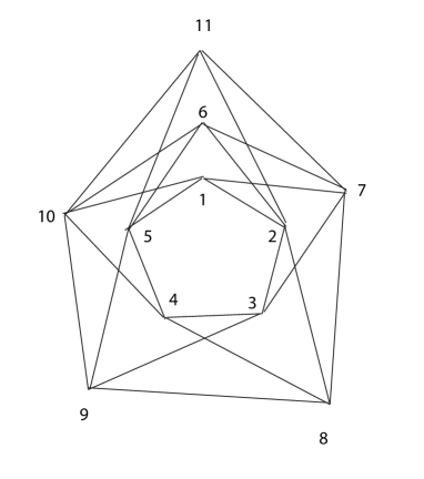
Figure 1: Left graph on 11 nodes has only 7 linearly independent odd holes. Right graph on 25 nodes has 25 linearly independent odd holes. Both graphs have no 3-cycles.

Left graph in Figure 1 below gives an example of $\bar{G}$ on 11 nodes with more than 11 cordless odd cycles but only 7 of them are independent. Active edge hypothesis is true on this graph or any subgraph of it or a super graph of it obtained by adding 3-cycles. However, it is possible to construct graphs with $n$ nodes and $n$ independent odd cycles and have no 3-cycles. Right graph in Figure 1 below gives such a graph on 25 nodes with no 3-cycles and 25 independent 5-cycles. The vector with $x_{i}=\frac{3}{5}$ for $i=1,2,\ldots 25$ is an optimal BFS of the ELP on this graph. If we encounter this BFS on this graph in the ELP reduction algorithm, we terminate with the flag that “active edge hypothesis failed”. It may be noted that there are alternative optimal BFS to this ELP relaxation which is integer. In fact solving this ELP using LINDO generated integer optimal solution {$x_{i}=0$, if $i=2,5,8,10,13,15,16,18,21,23;\ x_{i}=1$, otherwise} and not the fractional optimal solution we constructed above. Thus even if we encounter a situation where the active edge hypothesis is not satisfied in the algorithm, one may look for an active edge in an alternative optimal solution. Such a solution can be explored by forcing one of edge inequalities to be equality in the ELP and solving this modified ELP for each edge. At any stage, if the objective function value is not increased, then we have an alternative ELP solution with an active edge and the active edge reduction can be carried out.

3 Potpourri Extensions

Let us now discuss various techniques to handle the situation where the active edge hypothesis fails. These techniques provides minor improvements on the performance of the algorithm.

Random edge reduction: Remove an edge $(i,j)$ from $G$ along with its two incident nodes.

Without loss of generality assume $(i,j)=(n-1,n)$ and let $\bar{G}=G\setminus\{n-1,n\}.$ Let $x^{0}=(x_{1}^{0},x_{2}^{0},\ldots,x_{n}^{0})$ be an optimal BFS for the ELP on $G$ with objective function value $z(x^{0})$ and $\bar{x}=(\bar{x}_{1},\bar{x}_{2},\ldots\bar{x}_{n-2})$ be an optimal BFS for the ELP on $\bar{G}$ with optimal objective function value $\bar{z}(\bar{x})$.

Lemma 7

$\bar{z}(\bar{x})<z(x^{0})-1$.

Reduction operations in Algorithm ELP can easily be modified to incorporate the random edge reduction step. Unlike the active edge reduction, which chooses exactly one node from an active edge, the random edge reduction takes both nodes of the edge selected randomly. But the optimal vertex cover does not necessarily contain both these nodes and may contain only one of them. This is a 2-approximation. The active edge reduction and $\{0,1\}$-reduction however preserve optimality. Thus for each node selected in a $\{0,1\}$-reduction step or an active edge reduction step, we can perform one random edge reduction in the algorithm and still preserve the $\frac{3}{2}$-approximation guarantee. To improve the probability of a $\frac{3}{2}$-approximation guarantee, we want to make sure the total number of nodes collected in active edge reduction step and $\{0,1\}$-reduction step to be as large as possible. So it is better to perform an active edge reduction step in the ELP reduction algorithm before the three cycle reduction. To achieve this we want to make sure $(i,j)$ is not part of a 3-cycle in $G_{k}$, otherwise Lemma 3 is not valid. Fortunately, this is true since if $(i,j)$ is active and is part of a 3-cycle, the third node will have a value 1 in the ELP optimal solution and the $\{0,1\}$ reduction step would have removed this node. Consider the enhanced ELP Algorithm where Step 3 is replaced by:

• {* Reduction operations *} $\Delta_{k}=\emptyset$, $I_{k,1}=\emptyset,$ $(i_{k},j_{k})=\emptyset$, $(\bar{i}_{k},\bar{j}_{k})=\emptyset$, $(\hat{i}_{k},\hat{j}_{k})=\emptyset$.

  1. Let $I_{k,0}=\{i\ |\ x_{i}^{k}=0\},\ I_{k,1}=\{i\ |\ x_{i}^{k}=1\}$,
     If $|I_{k,1}|\neq\emptyset$ or $G_{k}$ has an active edge, goto Step 3 (3) endif

  2. {* Exploring alternate optimal BFS for active edge *} $E=E(G_{k})$, T=0,
     while $E\neq\emptyset$ do Choose an edge $(i,j)\in E$. Solve the ELP on $G_{k}$ with the edge inequality corresponding to $(i,j)$ replaced by an equality. Let $\tilde{x}$ be the optimal BFS obtained with the objective function value $\tilde{f}$.
     If $\tilde{f}=f^{k}$ then $x^{k}=\tilde{x},T=1$ and goto Step 3(3) else $E=E\setminus\{(i,j)\}$ endif
     endwhile
     If T=0, goto Step 3(5) endif

  3. {* {0,1}-reduction *} $I_{k}=I_{k,0}\cup I_{k,1}$.
     If $V(G_{k})\setminus I_{k}=\emptyset$, goto step 4, else $G_{k}=G_{k}\setminus I_{k}$ endif

  4. {* active edge reduction *}  If $G_{k}$ has active edges then Choose an active edge $(i,j)$. Let $G_{k+1}=G_{k}^{(i,j)}$ where $G_{k}^{(i,j)}$ is the graph obtained from $G_{k}$ using active edge reduction operation. Let $i_{k}=i,j_{k}=j$; $k=k+1$ goto Step 2 endif

  5. {* 3-cycle reduction *} If $G_{k}$ has 3-cycles then
     Choose a 3-cycle $\Delta_{k}$. Set $G_{k+1}=G_{k}\backslash\Delta_{k}$; $k=k+1,$ goto Step 2 endif

  6. {* over-active edge reduction *} If $G_{k}$ has over-active edges then
     Choose an over-active edge $(i,j)$. Set $G_{k+1}=G_{k}\backslash\{i,j\}$, and $\bar{i}_{k}=i,\bar{j}_{k}=j$; $k=k+1,$ goto Step 2 endif

  7. {* random edge reduction *} If the active edge hypothesis does not hold for $G_{k}$ then choose any edge $(i,j)$. Let $G_{k+1}=G_{k}\backslash\{i,j\}$, and $\hat{i}_{k}=i,\hat{j}_{k}=j$; $k=k+1$ goto Step 2 endif

Let $I_{1}=\cup_{k=1}^{L}I_{k,1}$ and $\eta,\gamma,\delta,\sigma$ be the number of active-edge reductions, random-edge reductions, 3-cycle reductions and over-active edge reductions, respectively, performed in the enhanced ELP algorithm. Let $\beta=|I_{1}|+\eta$, $\alpha=\max\{0,\gamma-\beta\}$ and $\lambda=\gamma+\delta+\frac{2}{3}\sigma$.

Lemma 8

The enhanced ELP computes a vertex cover $S_{1}$ on $G$ in polynomial time such that $|S_{1}|\leq\frac{3}{2}|S^{*}|+\frac{\alpha}{2}$, where $S^{*}$ is an optimal vertex cover on $G$. Further, $|S_{1}|\leq|S^{*}|+\lambda.$

Thus when $\alpha=0$ the enhanced ELP algorithm computes a $\frac{3}{2}$-approximate solution. When $\lambda=0$ the enhanced ELP algorithm computes an optimal solution. Recall that $f^{1}$ is the optimal objective function value of ELP on $G$. Note that $S_{1}$ has at most $\lambda$ extra nodes compared to an optimal vertex cover. Thus if $\lambda\leq\frac{f^{1}}{2}$ then,

$$|S_{1}|\leq|S^{*}|+\lambda\leq|S^{*}|+\frac{f^{1}}{2}\leq|S^{*}|+\frac{|S^{*}|}{2}=\frac{3}{2}|S^{*}|.$$

Let $\xi=\min\{\frac{\alpha}{2},\max\{0,\lambda-\frac{f^{1}}{2}\}\}$.

Theorem 3

The enhanced ELP algorithm computes a vertex cover $S_{1}$ on $G$ in polynomial time such that $|S_{1}|\leq\frac{3}{2}|S^{*}|+\xi$, where $S^{*}$ is an optimal vertex cover on $G$.

4 Conclusion

In this paper, we presented a polynomial time approximation algorithm that computes a vertex cover $S_{1}$ such that $|S_{1}|\leq\frac{3}{2}|S^{*}|+\xi$, where $S^{*}$ is an optimal vertex cover and $\xi$ is an error factor identified by the algorithm. In all the examples we constructed $\xi$ turned out to be zero. It would be interesting to compute explicit examples where $\xi\neq 0$.

It seems that the ELP Algorithm may not guarantee a $\frac{3}{2}$-approximate solution for VCP on all graphs, since it is based on the optimal objective function value of the ELP relaxation and the integrality gap of the ELP is basically 2 [1]. The proof in [1] is probabilistic in nature and establishes existence of a graph for which integrality gap is 2. No constructive proof of this is known. The operation of active edge reduction is crucial to our algorithm. Let $x^{0}$ be an optimal solution to the ELP problem, an edge $(i,j)$ is said to be a small edge with respect to $x^{0}$ if $x_{i}^{0}+x_{j}^{0}=\min\{x_{r}^{0}+x_{s}^{0}\ |\ (r,s)\in E(G)\}$. If an active edge exists in $G$ with respect to $x^{0}$, then it will be a small edge. If $G$ has no 3-cycles and $(i,j)$ is a small edge, one may be tempted to conjecture that there exists an optimal vertex cover $V^{0}$ of $G$ containing only one of the nodes in $\{i,j\}$. It turns out that this is true for a large class of graphs. If it is true in general, then it leads to a polynomial time $\frac{3}{2}$-approximation algorithm for VCP on any graph $G$.

Figure 2: A graph on 25 nodes with no 3-cycles such that both end nodes of all small edges are in all optimal vertex covers.

However, we have a very interesting counter example (See Figure 2) for this establishing that such a claim is not necessarily true. There are five different optimal vertex covers for the graph given in Figure 2 which are listed below:

$${\footnotesize\begin{array}[]{ccccccccccccccccccccccccc}1&2&3&4&5&6&7&8&9&10&11&12&13&14&15&16&17&18&19&20&21&22&23&24&25\\ \hline\cr 1&0&1&0&1&1&0&1&0&1&0&1&1&0&1&1&0&1&0&1&1&0&1&1&1\\ 1&0&1&0&1&1&0&1&0&1&1&0&1&0&1&1&0&1&0&1&1&0&1&1&1\\ 1&0&1&1&0&1&0&1&1&0&1&0&1&1&0&1&0&1&1&1&1&0&1&0&1\\ 1&0&1&1&0&1&0&1&1&0&1&0&1&1&1&1&0&1&0&1&1&0&1&0&1\\ 1&0&1&1&0&1&0&1&1&1&1&0&1&0&1&1&0&1&0&1&1&0&1&0&1\end{array}}$$

The unique optimal solution $x^{0}=(x_{1}^{0},x_{2}^{0},\cdots,x_{n}^{0})$ to ELP is given by $x^{0}_{i}=\frac{3}{5}$ for all $i$. Thus any edge is a small edge. If the small edge is selected as any of the following: $(1,21),(3,16),(3,18),(3,23)$, $(16,20),(16,25),(21,25)$, both of their incident nodes are in all optimal vertex covers.

Note that this graph is maximal without 3-cycles on 25 nodes, in the sense of that any additional edge will result in a 3-cycle in the graph. The graph discussed above does not satisfy active edge hypothesis. Nevertheless, the ELP Algorithm with extensions discussed in Section 3 guarantees a $\frac{3}{2}$-approximate solution for this graph, since only two random edge reductions are needed by following appropriate general rules that selects $(24,25),(22,23)$ for the operation of random edge reduction.

Acknowledgement: This work was partially supported by an NSERC discovery grant awarded to Abraham P. Punnen. The first author would be very grateful to Dr. Jiawei Zhang and Dr. Donglei Du for several helpful discussions.

References

- [1] S. Arora, B. Bollobs and L. Lovsz, Proving integrality gaps without knowing the linear program, Proc. IEEE FOCS (2002), 313-322.
- [2] E. Asgeirsson and C. Stein, Vertex cover approximations on random graphs, Lecture notes in computer science, Volume 4525 (2007) 285-296 Springer Verlag.
- [3] E. Asgeirsson and C. Stein, Vertex cover approximations: Experiments and observations, WEA, 545-557 (2005).
- [4] R. Bar-Yehuda and S. Even, A local-ratio theorem for approximating the weighted vertex cover problem, Annals of Discrete Mathematics, 25(1985), 27-45.
- [5] Moses Charikar, On semidefinite programming relaxations for graph coloring and vertex cover, Proc. 13th SODA (2002), 616-620.
- [6] I. Dinur and S. Safra, The importance of being biased, Proc. 34th ACM Symposium on Theory of Computing, 33-42, 2002.
- [7] Eran Halperin, Improved approximation algorithms for the vertex cover problem in graphs and hypergraphs, SIAM J. Comput., 31(2002), 1608-1623.
- [8] B. Harb, The unique games conjecture and some of its implications on inapproximability. Manuscript, May 2005.
- [9] J. Håstad, Some optimal inapproximability results, JACM 48(2001), 798-859.
- [10] D. S. Hochbaum, Approximation algorithms for set covering and vertex cover problems, SIAM J. Comput., 11(1982), 555-556.
- [11] D. S. Hochbaum, Approximating covering and packing problems: set cover, independent set, and related problems, in Approximation Algorithms for NP-Hard Problems, 94-143, edited by D. S. Hochbaum, PWS Publishing Company, 1997.
- [12] G. Karakostas, A better approximation ratio for the vertex cover problem, L. Caires et al. (Eds): ICALP 2005, LNCS 3580, 1043-1050.
- [13] S. Khot, On the power of unique 2-Prover 1-Round games. In proceedings of 34th ACM symposium on Theory of Computing (STOC) 767-775, 2002.
- [14] S. Khot and O. Regev, Vertex cover might be hard to approximate to within . Manuscript.
- [15] J. Kleinberg and M. Goemans, The Lovsz theta function and a semidefinite programming relaxation of vertex cover, SIAM J. Discrete Math., 11(1998), 196-204.
- [16] B. Monien, The complexity of determining a shortest cycle of even length, Computing, 31(1983), 355-369.
- [17] B. Monien and E. Speckenmeyer, Ramsey numbers and an approximation algorithm for the vertex cover problem, Acta Informatica, 22(1985), 115-123.
- [18] G. L. Nemhauser and L. E. Trotter, Jr. , Vertex packings: Structural properties and algorithms. Mathematical Programming, 8(1975), 232-248.