On the approximability of the vertex cover and related problems

Abstract

In this paper we show that the problem of identifying an edge $(i,j)$ in a graph $G$ such that there exists an optimal vertex cover $S$ of $G$ containing exactly one of the nodes $i$ and $j$ is NP-hard. Such an edge is called a weak edge. We then develop a polynomial time approximation algorithm for the vertex cover problem with performance guarantee $2-\frac{1}{1+\sigma}$, where $\sigma$ is an upper bound on a measure related to a weak edge of a graph. Further, we discuss a new relaxation of the vertex cover problem which is used in our approximation algorithm to obtain smaller values of $\sigma$. We also obtain linear programming representations of the vertex cover problem for special graphs. Our results provide new insights into the approximability of the vertex cover problem - a long standing open problem.

Keywords: vertex cover problem, approximation algorithm, LP-relaxation, weak edge reduction, NP-complete problems

1 Introduction

Let $G=(V,E)$ be an undirected graph on the vertex set $V=\{1,2,\ldots,n\}$. A vertex cover of $G$ is a subset $S$ of $V$ such that each edge of $G$ has at least one endpoint in $S$. The vertex cover problem (VCP) is to compute a vertex cover of smallest cardinality in $G$. The VCP is NP-hard on an arbitrary graph but solvable in polynomial time on a bipartite graph. A vertex cover $S$ is said to be $\gamma$-optimal if $|S|\leq\gamma|S^{0}|$ where $\gamma\geq 1$ and $S^{0}$ is an optimal solution to the VCP.

It is well known that a 2-optimal vertex cover of a graph can be obtained in polynomial time by taking all the vertices of a maximal (not necessarily maximum) matching in the graph or rounding up the LP relaxation solution of an integer programming formulation [18]. There has been considerable work (see e.g. survey paper [11]) on the problem over the past 30 years on finding a polynomial-time approximation algorithm with an improved performance guarantee. The current best known bound on the performance ratio of a polynomial time approximation algorithm for VCP is $2-\Theta(\frac{1}{\sqrt{\log n}})$ [12]. It is also known that computing a $\gamma$-optimal solution in polynomial time for VCP is NP-Hard for any $1\leq\gamma\leq 10\sqrt{5}-21\simeq 1.36$ [6]. In fact, no polynomial-time $(2-\epsilon)$-approximation algorithm is known for VCP for any constant $\epsilon>0$ and existence of such an algorithm is one of the most outstanding open questions in approximation algorithms for combinatorial optimization problems. Under the assumption that the unique game conjecture [9, 13, 14] is true, many researchers believe that a polynomial time $(2-\epsilon)$-approximation algorithm with constant $\epsilon>0$ is not possible for VCP. For recent works on approximability of VCP, we refer to [1, 4, 5, 6, 7, 8, 10, 12, 15, 16]. Recently Asgeirsson and Stein [2, 3] reported extensive experimental results using a heuristic algorithm which obtained no worse than $\frac{3}{2}$-optimal solutions for all the test problems they considered. Also, Han, Punnen and Ye [8] proposed a $(\frac{3}{2}+\xi)$-approximation algorithm for VCP, where $\xi$ is an error parameter calculated by the algorithm and reported that no example was known where $\xi\neq 0$.

A natural integer programming formulation of VCP can be described as follows:

$$(IP)\hskip 15.0pt\begin{array}[]{lcl}&\min&\sum_{i=1}^{n}x_{i}\\ &s.t.&x_{i}+x_{j}\geq 1,(i,j)\in E,\\ &&x_{i}\in\{0,1\},i=1,2,\cdots,n.\end{array}$$ (1)

Let $\bar{x}=(\bar{x}_{1},\bar{x}_{2},\ldots,\bar{x}_{n})$ be an optimal solution to (1). Then $S_{IP}=\{i\ |\ \bar{x}_{i}=1\}$ is an optimal vertex cover of the graph $G$. The linear programming (LP) relaxation of the above integer program is

$$(LPR)\hskip 15.0pt\begin{array}[]{lcl}&\min&\sum_{i=1}^{n}x_{i}\\ &s.t.&x_{i}+x_{j}\geq 1,(i,j)\in E,\\ &&x_{i}\geq 0,i=1,2,\cdots,n.\end{array}$$ (2)

It is well known that (e.g. [17]) any optimal basic feasible solution (BFS) $x^{*}=(x^{*}_{1},x^{*}_{2},\ldots,x^{*}_{n})$ to the problem LPR, satisfies $x_{i}^{*}\in\{0,\frac{1}{2},1\}$. Let $S_{LP}=\{i\ |\ x_{i}^{*}=\frac{1}{2}\mbox{ or }x_{i}^{*}=1\}$, then it is easy to see that $S_{LP}$ is a $2$-approximate solution to the VCP on graph $G$. Nemhauser and Trotter [18] have further proved that there exists an optimal integer solution to (1), which agrees with $x^{*}$ in its integer components.

An $(i,j)\in E$ is said to be a weak edge if there exists an optimal vertex cover $V^{0}$ of $G$ such that $|V^{0}\cap\{i,j\}|=1$. Likewise, an $(i,j)\in E$ is said to be a strong edge if there exists an optimal vertex cover $V^{0}$ of $G$ such that $|V^{0}\cap\{i,j\}|=2$. An edge $(i,j)$ is uniformly strong if $|V^{0}\cap\{i,j\}|=2$ for any optimal vertex cover $V^{0}.$ Note that it is possible for an edge to be both strong and weak. Also $(i,j)$ is uniformly strong if and only if it is not a weak edge. In this paper, we show that the problems of identifying a weak edge and identifying a strong edge are NP-hard. We also present a polynomial time $(2-\frac{1}{\sigma+1})$-approximation algorithm for VCP where $\sigma$ is an appropriate graph theoretic measure (to be introduced in Section 3). Thus for all graphs for which $\sigma$ bounded above by a constant, we have a polynomial time $(2-\epsilon)$-approximation algorithm for VCP. So far we could not identify any class of graphs where $\sigma$ is anything but a constant. We also give examples of graphs satisfying the property that $\sigma=0$. However, establishing tight bounds on $\sigma$, independent of graph structures remains an open question. VCP is trivial on a complete graph $K_{n}$ since any collection of $n-1$ nodes serves as an optimal solution. However, the LPR gives an objective function value of $\frac{n}{2}$ only. We give a stronger relaxation for VCP and complete linear programming description of VCP on a complete graph, wheels, among others. This relaxation can also be used to find reasonable expected guarantee for $\sigma$.

For any graph $G$, we sometimes use the notation $V(G)$ to represent its vertex set and $E(G)$ to represent its edge set.

2 Complexity of weak and strong edge problems

The strong edge problem can be stated as follows: “Given a graph, identify a strong edge of $G$ or declare that no such edge exists.”

Theorem 1

The strong edge problem is NP-hard.

Proof. If $G$ is bipartite, then it does not contain a strong edge. If $G$ is not bipartite, then it must contain an odd cycle. For any odd cycle $\omega$, any vertex cover must contain at least two adjacent nodes of $\omega$ and hence $G$ must contain at least one strong edge. If such an edge $(i,j)$ can be identified in polynomial time, then after removing the nodes $i$ and $j$ from $G$ and applying the algorithm on $G-\{i,j\}$ and repeating the process we eventually reach a bipartite graph for which an optimal vertex cover $\hat{V}$ can be identified in polynomial time. Then $\hat{V}$ together with the nodes removed sofar will form an optimal vertex cover of $G$. Thus if the strong edge problem can be solved in polynomial time, then the VCP can be solved in polynomial time.   

The problem of identifying a weak edge is much more interesting. The weak edge problem can be stated as follows: “Given a graph $G$, identify a weak edge of $G$.” It may be noted that unlike a strong edge, a weak edge exists for all graphs. We will now show that the weak edge problem is NP-hard. Before discussing the proof of this, we need to introduce some notations and definitions.

Let $x^{*}=(x_{1}^{*},x_{2}^{*},\ldots,x_{n}^{*})$ be an optimal BFS of LPR, the linear programming relaxation of the VCP. Let $I_{0}=\{i~{}:~{}x^{*}_{i}=0\}$ and $I_{1}=\{i~{}:~{}x_{i}^{*}=1\}$. The graph $\bar{G}=G\setminus\{I_{0}\cup I_{1}\}$ is called the $\{0,1\}$-reduced graph of $G$. The process of computing $\bar{G}$ from $G$ is called a {0,1}-reduction.

Lemma 1

[18] If $R$ is a vertex cover of $\bar{G}$ then $R\cup I_{1}$ is a vertex cover of $G$. If $R$ is optimal for $\bar{G}$, then $R\cup I_{1}$ is an optimal vertex cover for $G$. If $R$ is an $\gamma$-optimal vertex cover of $\bar{G}$, then $R\cup I_{1}$ is an $\gamma$-optimal vertex cover of $G$ for any $\gamma\geq 1$.

Let $(i,j)$ be an edge of $G$. Define $\Delta_{ij}=\{k\ |\ (i,k)\in E(G)\mbox{ and }(j,k)\in E(G)\}$, $D_{i}=\{s\in V(G)\ |\ (i,s)\in E(G),s\not=j,s\not\in\Delta_{ij}\}$, and $D_{j}=\{t\in V(G)\ |\ (j,t)\in E(G),t\not=i,t\not\in\Delta_{ij}\}$. Construct the new graph $G^{(i,j)}$ from $G$ as follows. From graph $G,$ delete $\Delta_{ij}$ and all the incident edges, connect each vertex $s\in D_{i}$ to each vertex $t\in D_{j}$ whenever such an edge is not already present, and delete vertices $i$ and $j$ with all the incident edges. The operation of constructing $G^{(i,j)}$ from $G$ is called an $(i,j)$-reduction. When $(i,j)$ is selected as a weak edge, then the corresponding $(i,j)$-reduction is called a weak edge reduction. The weak edge reduction is a modified version of the active edge reduction operation introduced in [8].

Figure 1: Weak edge reduction using edge $(1,2)$. $D_{1}=\{8,4\}$, $D_{2}=\{7\}$ and $\Delta_{12}=\{3,5\}$. The graph $G^{(1,2)}$ is on the right.

Lemma 2

Let $(i,j)$ be a weak edge of $G$, $R\subseteq V(G^{(i,j)})$ and

$$R^{*}=\begin{cases}R\cup\Delta_{ij}\cup\{j\},&\text{ if }D_{i}\subseteq R;\\ R\cup\Delta_{ij}\cup\{i\},&\text{ otherwise},\end{cases}$$

1. If $R$ is a vertex cover of $G^{(i,j)}$, then $R^{*}$ is a vertex cover of $G$.

2. If $R$ is an optimal vertex cover of $G^{(i,j)}$, then $R^{*}$ is an optimal vertex cover of $G$.

3. If $R$ is a $\gamma$-optimal vertex cover in $G^{(i,j)}$, then $R^{*}$ is a $\gamma$-optimal vertex cover in $G$ for any $\gamma\geq 1$.

Proof. If $D_{i}\subseteq R$ then all arcs in $G$ incident on $i,$ except possibly $(i,j),$ is covered by $R$. Then $R^{*}=R\cup\Delta_{ij}\cup\{j\}$ covers all arcs incident on $j$, including $(i,j)$ and hence $R^{*}$ is a vertex cover in $G$. If at least one vertex of $D_{i}$ is not in $R$, then all vertices in $D_{j}$ must be in $R$ by construction of $G^{(i,j)}$. Thus $R^{*}=R\cup\Delta_{ij}\cup\{i\}$ must be a vertex cover of $G$.

Suppose $R$ is an optimal vertex cover of $G^{(i,j)}$. Since $(i,j)$ is a weak edge, there exists an optimal vertex cover, say $V^{0}$, of $G$ containing exactly one of the nodes $i$ or $j$. Without loss of generality, let this node be $i$. For each node $k\in\Delta_{ij}$, $(i,j,k)$ is a 3-cycle in $G$ and hence $k\in V^{0}$ for all $k\in\Delta_{ij}$. Let $V^{1}=V^{0}-(\{i\}\cup\Delta_{ij})$, which is a vertex cover of $G^{(i,j)}$. Then $|R|=|V^{1}|$ for otherwise if $|R|<|V^{1}|$ we have $|R^{*}|<|V^{0}|$, a contradiction. Thus $|R^{*}|=|V^{0}|$ establishing optimality of $R^{*}$.

Suppose $R$ is an $\gamma$-optimal vertex cover of $G^{(i,j)}$ and let $V^{(i,j)}$ be an optimal vertex cover in $G^{(i,j)}$. Thus

$$|R|\leq\gamma|V^{(i,j)}|\mbox{ where }\gamma\geq 1.$$ (3)

Let $V^{0}$ be an optimal vertex cover in $G$. Without loss of generality assume $i\in V^{0}$ and since $(i,j)$ is weak, $j\notin V^{0}.$ Let $V^{1}=V^{0}-(\{i\}\cup\Delta_{ij}).$ Then $|V^{1}|=|V^{(i,j)}|.$ Thus we from (3), $|R|\leq\gamma|V^{1}|.$ Thus

$$|R^{*}|\leq\gamma|V^{1}|+|\Delta_{ij}|+1\leq\gamma(|V^{1}|+|\Delta_{ij}|+1)\leq\gamma|V^{0}|.$$

Thus $R^{*}$ is $\gamma$-optimal in $G.$   

Suppose that an oracle, say WEAK($G,i,j$), is available which with input $G$ outputs two nodes $i$ and $j$ such that $(i,j)$ is a weak edge of $G$. It may be noted that WEAK($G,i,j$) do not tell us which node amongst $i$ and $j$ is in an optimal vertex cover. It simply identifies the weak edge $(i,j)$. Using the oracle WEAK($G,i,j$), we develop an algorithm, called weak edge reduction algorithm or WER-algorithm to compute an optimal vertex cover of $G$.

The basic idea of the scheme is very simple. We apply $\{0,1\}$ and weak edge reductions repeatedly until a null graph is reached, in which case the algorithm goes to a backtracking step. We record the vertices of the weak edge identified in each weak edge reduction step but do not determine which one to be included in the output vertex cover. In the backtrack step, taking guidance from lemma 2, we choose exactly one of these two vertices to form part of the vertex cover we construct. In this step, the algorithm computes a vertex cover for $G$ using all vertices in $\Delta_{ij}$ removed in the weak edge reduction steps, vertices with value 1 removed in the $\{0,1\}$ reduction steps, and the selected vertices in the backtrack step from the vertices corresponding to the weak edges recorded during the weak edge reduction steps. A formal description of the WER-algorithm is given below.

• The WER-Algorithm

• {* Initialize *} $k=1,G_{k}=G$.

• {* Reduction operations *} $\Delta_{k}=\emptyset$, $I_{k,1}=\emptyset,$ $(i_{k},j_{k})=\emptyset$.

  1. {* {0,1}-reduction *} Solve the LP relaxation problem LPR of VCP on the graph $G_{k}$. Let $x^{k}=\{x_{i}^{k}:i\in V(G_{k})\}$ be the resulting optimal BFS, $I_{k,0}=\{i\ |\ x_{i}^{k}=0\},\ I_{k,1}=\{i\ |\ x_{i}^{k}=1\}$, and $I_{k}=I_{k,0}\cup I_{k,1}$.
     If $V(G_{k})\setminus I_{k}=\emptyset$ goto Step 3 else $G_{k}=G_{k}\setminus I_{k}$ endif

  2. {* weak edge reduction *} Call WEAK($G_{k},i,j$) to identify the weak edge $(i,j)$. Let $G_{k+1}=G_{k}^{(i,j)}$, where $G_{k}^{(i,j)}$ is the graph obtained from $G_{k}$ using the weak edge reduction operation. Compute $\Delta_{ij}$ for $G_{k}$ as defined in the weak edge reduction. Let $\Delta_{k}=\Delta_{ij},i_{k}=i,j_{k}=j$.
     If $G_{k+1}\not=\emptyset$ then $k=k+1$ goto beginning of Step 2 endif

• L=k+1, $S_{L}=\emptyset$.

• {* Backtracking to construct a solution *}
  Let $S_{L-1}=S_{L}\cup I_{L-1,1}$,
  If $(i_{L-1},j_{L-1})\neq\emptyset$ then $S_{L-1}=S_{L-1}\cup\Delta_{L-1}\cup R^{*}$, where

  $$R^{*}=\begin{cases}j_{L-1},&\text{ if }D_{i_{L-1}}\subseteq S_{L};\\ i_{L-1},&\text{ otherwise},\end{cases}$$

    and $D_{i_{L-1}}=\{s:(i_{L-1},s)\in G_{L-1},s\neq j_{L-1},s\not\in\Delta_{L-1}\}$ endif
  $L=L-1$,
  If $L\neq 1$ then goto beginning of step 4 else output $S_{1}$ and STOP endif

Using Lemma 1 and Lemma 2, it can be verified that the output $S_{1}$ of the WER-algorithm is an optimal vertex cover of $G$. It is easy to verify that the complexity of the algorithm is polynomial whenever the complexity of WEAK($G,i,j$) is polynomial. Since VCP is NP-hard we established the following theorem:

Theorem 2

The weak edge problem is NP-hard.

3 An approximation algorithm for VCP

Let VCP($i,j$) be the restricted vertex cover problem where feasible solutions are vertex covers of $G$ using exactly one of the vertices from the set $\{i,j\}$ and looking for the smallest vertex cover satisfying this property. More precisely, VCP($i,j$) tries to identify a vertex cover $V^{*}$ of $G$ with smallest cardinality such that $|V^{*}\cap\{i,j\}|=1.$ Let $\delta$ and $\bar{\delta}(i,j)$ be the optimal objective function values of VCP and VCP($i,j$) respectively. If $(i,j)$ is indeed a weak edge of $G$, then $\delta=\bar{\delta}(i,j)$. Otherwise,

$$\bar{\delta}(i,j)=\delta+\sigma(i,j),$$ (4)

where $\sigma(i,j)$ is a non-negative integer. Further, using arguments similar to the proof of Lemma 2 it can be shown that

$$\zeta_{ij}+\Delta_{ij}+1=\bar{\delta}(i,j)=\delta+\sigma(i,j).$$ (5)

where $\zeta_{ij}$ is the optimal objective function value VCP on $G^{(i,j)}$.

Consider the optimization problem

WEAK-OPT:	Minimize $\sigma(i,j)$
	Subject to $(i,j)\in E(G)$

WEAK-OPT is precisely the weak edge problem in the optimization form and its optimal objective function value is always zero. However this problem is NP-hard by Theorem 2. We now show that an upper bound $\sigma$ on the optimal objective function value of WEAK-OPT and a solution $(i,j)$ with $\sigma(i,j)\leq\sigma$ can be used to obtain a $(2-\frac{1}{1+\sigma})$-approximation algorithm for VCP. Let ALMOST-WEAK($G,i,j$) be an oracle which with input $G$ computes an approximate solution $(i,j)$ to WEAK-OPT such that $\sigma(i,j)\leq\sigma$ for some $\sigma$. Consider the WER-algorithm with WEAK($G,i,j$) replaced by ALMOST-WEAK($G,i,j$). We call this the AWER-algorithm.

Let $G_{k},~{}k=1,2,\ldots t$ be the sequence of graphs generated in Step 2(2) of the AWER-algorithm and $(i_{k},j_{k})$ be the approximate solution to WEAK-OPT on $G_{k},~{}k=1,2,\ldots,t$ identified by ALMOST-WEAK($G_{k},i_{k},j_{k}$).

Theorem 3

The AWER-algorithm identifies a vertex cover $S_{1}$ such that $|S_{1}|\leq(2-\frac{1}{1+\sigma})|S^{*}|$ where $S^{*}$ is an optimal solution to the VCP. Further, the complexity of the the algorithm is $O(n(\phi(n)+\psi(n))$ where $n=|V(G)|$, $\phi(n)$ is the complexity of LPR and $\psi(n)$ is the complexity of ALMOST-WEAK($G,i,j$).

Proof. Without loss of generality, we assume that the LPR solution $x^{1}=(x_{1}^{1},x^{1}_{2},\ldots,x^{1}_{n})$ generated when Step 2(1) is executed for the first time satisfies $x^{1}_{i}=\frac{1}{2}$ for all $i$. If this is not true, then we could replace $G$ by a new graph $\bar{G}=G\setminus\{I_{1,1}\cup I_{1,0}\}$ and by Lemma 1, if $\bar{S}$ is a $\gamma$-optimal solution for VCP on $\bar{G}$ then $\bar{S}\cup I_{1,1}$ is a $\gamma$-optimal solution on $G$ for any $\gamma\geq 1$. Thus, under this assumption we have

$$n\leq 2|S^{*}|.$$ (6)

Let $t$ be the total number of iterations of Step 2 (2). For simplicity of notation, we denote $\sigma_{k}=\sigma(i_{k},j_{k})$ and $\bar{\delta}_{k}=\bar{\delta}(i_{k},j_{k})$. Note that $\delta_{k}$ and $\bar{\delta_{k}}$ are optimal objective function values of VCP and VCP($i_{k},j_{k}$), respectively, on the graph $G_{k}$. In view of equations (4) and (5) we have,

$$\bar{\delta}_{k}=\delta_{k}+\sigma_{k},~{}~{}~{}~{}~{}k=1,2,\ldots,t$$ (7)

and

$$\delta_{k+1}+|\Delta_{i_{k},j_{k}}|+|I_{k,1}|+1=\bar{\delta}_{k},~{}~{}~{}~{}~{}k=1,2,\ldots,t.$$ (8)

From (7) and (8) we have

$$\delta_{k+1}-\delta_{k}=\sigma_{k}-|\Delta_{i_{k},j_{k}}|-|I_{k,1}|-1,~{}~{}~{}k=1,2,\ldots,t.$$ (9)

Adding equations in (9) for $k=1,2,\ldots,t$ and using the fact that $\delta_{t+1}=|I_{t+1,1}|$, we have,

$$|S_{1}|=|S^{*}|+\sum_{k=1}^{t}\sigma_{k},$$ (10)

where $|S^{*}|=\delta_{1}$, and by construction,

$$|S_{1}|=\Sigma_{k=1}^{t+1}I_{k,1}+\Sigma_{k=1}^{t}\Delta_{k}+t.$$ (11)

But,

$$|V(G)|=\Sigma_{k=1}^{t+1}I_{k}+\Sigma_{k=1}^{t}\Delta_{k}+2t.$$ (12)

From (10), (11) and (12), we have

$$t=\frac{|V(G)|-\Sigma_{k=1}^{t+1}I_{k}-\Sigma_{k=1}^{t}\Delta_{k}}{2}\leq\frac{|V(G)|-|S^{*}|-\Sigma_{k=1}^{t}(\sigma_{k}-1)}{2}.$$ (13)

From inequalities (6) and (13), we have

$$t\leq\frac{|S^{*}|-t(\bar{\sigma}-1)}{2},$$

where $\bar{\sigma}=\frac{\Sigma_{k=1}^{t}\sigma_{k}}{t}$. Then we have

$$t\leq\frac{|S^{*}|}{\bar{\sigma}+1}.$$

Thus,

$$\frac{|S_{1}|}{|S^{*}|}=\frac{|S^{*}|+\Sigma_{k=1}^{t}\sigma_{k}}{|S^{*}|}=\frac{|S^{*}|+t\bar{\sigma}}{|S^{*}|}\leq 1+\frac{\bar{\sigma}}{\bar{\sigma}+1}\leq 1+\frac{\sigma}{\sigma+1}=2-\frac{1}{1+\sigma}.$$

The complexity of the algorithm can easily be verified.   

The performance bound established in Theorem 3 is useful only if we can find an efficient way to implement our black-box oracle ALMOST-WEAK($G,i,j$) that identifies a reasonable $(i,j)$ in each iteration. If ALMOST-WEAK($G,i,j)$ simply generates a random edge, then $\sigma(i,j)$ could be as large as $O(n)$ as given in the example of Figure 2.

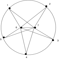
Figure 2: A 3D-wheel with central axis (6, 7).

For a 3D-wheel on $n$ nodes with central axis $(n-1,n)$, $\sigma(n-1,n)=\lfloor\{\frac{n}{2}\}-2\rfloor$. However, when $(i,j)$ is chosen as any other edge, $\sigma(i,j)=0$. A trivial upper bound on $\sigma$ is $\frac{n}{2}$ for any graph on $n$ nodes. Let us now explore the possibilities of improving this trivial bound.

Any vertex cover must contain at least $s+1$ vertices of an odd cycle of length $2s+1$. This motivates the following extended linear programming relaxation (ELP) of the VCP, studied in [1, 8].

$$(ELP)\hskip 10.0pt\begin{array}[]{lcl}&\min&{\displaystyle\sum_{i=1}^{n}x_{i}}\\ &s.t.&x_{i}+x_{j}\geq 1,(i,j)\in E,\\ &&{\displaystyle\sum_{i\in\omega_{k}}x_{i}\geq s_{k}+1,\omega_{k}\in\Omega,}\\ &&x_{i}\geq 0,i=1,2,\ldots,n,\end{array}$$ (14)

where $\Omega$ denotes the set of all odd-cycles of $G$ and $\omega_{k}\in\Omega$ contains $2s_{k}+1$ vertices for some integer $s_{k}$. Note that although there may be an exponential number of odd-cycles in $G$, since the odd cycle inequalities has a polynomial-time separation scheme, ELP is polynomially solvable. Further, it is possible to compute an optimal BFS of ELP in polynomial time.

Let $x^{0}$ be an optimal basic feasible solution of ELP. An edge $(r,s)\in E$ is said to be an active edge with respect to $x^{0}$ if $x^{0}_{i}+x^{0}_{j}=1$. There may or may not exist an active edge corresponding to an optimal BFS of the ELP as shown in [8]. For any arc $(r,s)$, consider the restricted ELP (RELP($r,s$)) as follows:

$$(RELP(r,s))\hskip 15.0pt\begin{array}[]{lcl}&\min&{\displaystyle\sum_{i=1}^{n}x_{i}}\\ &s.t.&x_{i}+x_{j}\geq 1,(i,j)\in E\backslash\{(r,s)\},\\ &&x_{r}+x_{s}=1,\\ &&{\displaystyle\sum_{i\in\omega_{k}}x_{i}\geq s_{k}+1,\omega_{k}\in\Omega,}\\ &&x_{i}\geq 0,i=1,2,\ldots,n,\end{array}$$ (15)

Let $Z(r,s)$ be the optimal objective function value of RELP($r,s$). Choose $(p,q)\in E(G)$ such that

$$\quad\quad\quad Z(p,q)=\min\{Z(i,j)~{}:~{}(i,j)\in E(G)\}.$$

An optimal solution to RELP($p,q$) is called a RELP solution. It may be noted that if an optimal solution $x^{*}$ of the ELP contains an active edge, then $x^{*}$ is also an RELP solution. Further $Z(p,q)$ is a lower bound on the optimal objective function value of VCP.

The VCP on a complete graph is trivial since any collection of $(n-1)$ nodes form an optimal vertex cover. However, for a complete graph, LPR yields an optimal objective function value of $\frac{n}{2}$ only and ELP yields an optimal objective function value of $\frac{2n}{3}$. Interestingly, the optimal objective function value of RELP on a complete graph is $n-1$, and the RELP solution is indeed an optimal vertex cover on a complete graph. A stronger version of this observation is proved in the following theorem.

Theorem 4

For any $(i,j)\in E(G),$ an optimal BFS of the linear program RELP($i,j$) gives an optimal vertex cover of $G$ whenever $G$ is a complete graph or a wheel.

Proof. Suppose $G$ is a complete graph with $V(G)=\{1,2,\ldots,n\}.$ Without loss of generality assume $(i,j)=(1,2)$. Thus

$$x^{0}_{1}+x^{0}_{2}=1.$$ (16)

Let $x^{0}=(x_{1}^{0},x_{2}^{0},\ldots,x_{n}^{0})$ be an optimal basic solution of RELP($i,j$). Since $x_{1}^{0}+x_{2}^{0}=1,$ by odd cycle inequalities, we have

$$x_{1}^{0}+x_{2}^{0}+x_{k}^{0}=2,~{}~{}~{}k=2,3,\ldots,n.$$ (17)

Hence $x_{k}^{0}=1$ for $k=3,4,\ldots,n$ yielding $Z(i,j)=n-1$. Now we have to establish that $x^{0}_{1}$ and $x^{0}_{2}$ cannot be fractional. If $x^{0}_{1}+x^{0}_{r}+x^{0}_{s}=2$ for any $\{r,s\}\neq\{1,2\}$ then $x^{0}_{1}=0$ yielding $x^{0}_{2}=1$. Similarly if $x^{0}_{2}+x^{0}_{r}+x^{0}_{s}=2$ for any $\{r,s\}\neq\{1,2\}$ then $x^{0}_{2}=0$ yielding $x^{0}_{1}=1$. If $x^{0}_{r}+x^{0}_{s}+x^{0}_{t}>2$ for all 3-cycles other than those in (17) it can be shown that there must exist an edge inequality, other than (16), satisfied as an equality. Such an equality must be of the form $x^{0}_{1}+x^{0}_{r}=1$ or $x^{0}_{2}+x^{0}_{r}=1$ for $r\in\{3,4,\ldots,n\}$ and hence $x^{0}_{1}$ and $x^{0}_{2}$ can take only values zero or one. Both $\{2,3,\ldots,n\}$ and $\{1,3,\ldots,n\}$ are optimal vertex covers for $G$. The proof for the case of a wheel can be obtained using similar analysis and we skip the details.   

It may be noted that an optimal BFS of RELP($i,j$) gives an optimal vertex cover on a 3D-wheel (Figure 2) when $(i,j)$ is not the central axis.

Extending the notion of an active edge corresponding to an ELP solution [8], an edge $(i,j)\in E$ is said to be an active edge with respect to an RELP solution $x^{0}$ if $x^{0}_{i}+x^{0}_{j}=1$. Unlike ELP, an RELP solution always contains an active edge. In AWER-algorithm, the output of ALMOST-WEAK($G,i,j$) can be selected as an active edge with respect to a RELP solution on $G$.

We believe that the value of $\sigma(i,j)$, i.e. the absolute difference between the optimal objective function value of VCP and the optimal objective function value of VCP($i,j$), when $(i,j)$ is an active edge corresponding to an RELP solution is a constant with very high probability, if not with probability one. If it is a constant, then our algorithm resolves the long standing question on the existence of a polynomial time $2-\epsilon$ approximation algorithm for VCP for constant $\epsilon>0.$ It is an open question to obtain a tight bound, deterministic or probabilistic, on this interesting graph theoretic measure. Nevertheless, our results provide new insight into the approximability of the vertex cover problem.

4 Conclusion

In this paper, we proved that weak edge and strong edge problems are NP-hard. We also presented a polynomial time $(2-\frac{1}{\sigma+1})$-approximation algorithm for VCP where $\sigma$ is a well defined graph theoretic measure. Obtaining tight upper bounds on $\sigma,$ deterministic or probabilistic, is an open question. We also provide simple linear programming representation of VCP on a complete graph, wheel and 3D-wheel, among other graphs.

Acknowledgements: Research of Qiaoming Han was supported in part by Chinese NNSF grant, and the Return-from-Abroad foundation of MOE China. Research of Abraham P. Punnen is partially supported by an NSERC discovery grant.

References

- [1] S. Arora, B. Bollobs and L. Lovsz, Proving integrality gaps without knowing the linear program, Proc. IEEE FOCS (2002), 313-322.
- [2] E. Asgeirsson and C. Stein, Vertex cover approximations on random graphs, Lecture notes in computer science, Volume 4525 (2007) 285-296 Springer Verlag.
- [3] E. Asgeirsson and C. Stein, Vertex cover approximations: Experiments and observations, WEA, 545-557 (2005).
- [4] R. Bar-Yehuda and S. Even, A local-ratio theorem for approximating the weighted vertex cover problem, Annals of Discrete Mathematics, 25(1985), 27-45.
- [5] Moses Charikar, On semidefinite programming relaxations for graph coloring and vertex cover, Proc. 13th SODA (2002), 616-620.
- [6] I. Dinur and S. Safra, The importance of being biased, Proc. 34th ACM Symposium on Theory of Computing, 33-42, 2002.
- [7] Eran Halperin, Improved approximation algorithms for the vertex cover problem in graphs and hypergraphs, SIAM J. Comput., 31(2002), 1608-1623.
- [8] Q. Han, A.P. Punnen and Y. Ye, A polynomial time -approximation algorithm for the vertex cover problem on a class of graphs, Working paper, 2007.
- [9] B. Harb, The unique games conjecture and some of its implications on inapproximability. Manuscript, May 2005.
- [10] J. Håstad, Some optimal inapproximability results, JACM 48(2001), 798-859.
- [11] D. S. Hochbaum, Approximating covering and packing problems: set cover, independent set, and related problems, in Approximation Algorithms for NP-Hard Problems, 94-143, edited by D. S. Hochbaum, PWS Publishing Company, 1997.
- [12] G. Karakostas, A better approximation ratio for the vertex cover problem, L. Caires et al. (Eds): ICALP 2005, LNCS 3580, 1043-1050.
- [13] S. Khot, On the power of unique 2-Prover 1-Round games. In proceedings of 34th ACM symposium on Theory of Computing (STOC) 767-775, 2002.
- [14] S. Khot and O. Regev, Vertex cover might be hard to approximate to within . Manuscript.
- [15] J. Kleinberg and M. Goemans, The Lovsz theta function and a semidefinite programming relaxation of vertex cover, SIAM J. Discrete Math., 11(1998), 196-204.
- [16] B. Monien and E. Speckenmeyer, Ramsey numbers and an approximation algorithm for the vertex cover problem, Acta Informatica, 22(1985), 115-123.
- [17] G. L. Nemhauser and L. E. Trotter, Jr. , Properties of vertex packing and independence system polyhedra, Mathematical Programming, 6(1974), 48-61.
- [18] G. L. Nemhauser and L. E. Trotter, Jr. , Vertex packings: Structural properties and algorithms. Mathematical Programming, 8(1975), 232-248.