The Capacity Region of a Class of 3-Receiver Broadcast Channels with Degraded Message Sets

Abstract

Körner and Marton established the capacity region for the 2-receiver broadcast channel with degraded message sets. Recent results and conjectures suggest that a straightforward extension of the Körner-Marton region to more than 2 receivers is optimal. This paper shows that this is not the case. We establish the capacity region for a class of 3-receiver broadcast channels with 2 degraded message sets and show that it can be strictly larger than the straightforward extension of the Körner-Marton region. The key new idea is indirect decoding, whereby a receiver who cannot directly decode a cloud center, finds it indirectly by decoding satellite codewords. This idea is then used to establish new inner and outer bounds on the capacity region of the general 3-receiver broadcast channel with 2 and 3 degraded message sets. We show that these bounds are tight for some nontrivial cases. The results suggest that the capacity of the 3-receiver broadcast channel with degraded message sets is as at least as hard to find as the capacity of the general 2-receiver broadcast channel with common and private message.

I Introduction

A broadcast channel with degraded message sets represents a scenario where a sender wishes to communicate a common message to all receivers, a first private message to a first subset of the receivers, a second private message to a second subset of the first subset and so on. Such scenario can arise, for example, in video or music broadcasting over a wireless network to nested subsets of receivers at varying levels of quality. The common message represents the lowest quality version to be sent to all receivers, the first private message represents the additional information needed for the first subset of receivers to decode the second lowest quality version, and so on. What is the set of simultaneously achievable rates for communicating such degraded message sets over the network?

This question was first studied by Körner and Marton in 1977 [1]. They considered a general 2-receiver discrete-memoryless broadcast channel with sender $X$ and receivers $Y_{1}$ and $Y_{2}$. A common message $M_{0}\in[1,2^{nR_{0}}]$ is to be sent to both receivers and a private message $M_{1}\in[1,2^{nR_{1}}]$ is to be sent only to receiver $Y_{1}$. They showed that the capacity region is given by the set of all rate pairs $(R_{0},R_{1})$ such that 

$$R_{0} \leq\min\{I(U;Y_{1}),I(U;Y_{2})\},$$ (1)

$$R_{1} \leq I(X;Y_{1}|U),$$

for some $p(u,x)$. These rates are achieved using superposition coding [2]. The common message is represented by the auxiliary random variable $U$ and the private message is superimposed to generate $X$. The main contribution of [1] is proving a strong converse using the technique of images-of-a-set [3].

Extending the Körner-Marton result to more than 2 receivers has remained open even for the simple case of 3 receivers $Y_{1},Y_{2},Y_{3}$ with 2 degraded message sets, where a common message $M_{0}$ is to be sent to all receivers and a private message $M_{1}$ is to be sent only to receiver $Y_{1}$. The straightforward extension of the Körner-Marton region to this case yields the achievable rate region consisting of the set of all rate pairs $(R_{0},R_{1})$ such that

$$R_{0} \leq\min\{I(U;Y_{1}),I(U;Y_{2}),I(U;Y_{3})\},$$ (2)

$$R_{1} \leq I(X;Y_{1}|U),$$

for some $p(u,x)$. Is this region optimal?

In [4], it was shown that the above region (and its natural extension to $k>3$ receivers) is optimal for a class of product discrete-memoryless and Gaussian broadcast channels, where each of the receivers who decode only the common message is a degraded version of the unique receiver that also decodes the private message. In [5], it was shown that a straightforward extension of Körner-Marton region is optimal for the class of linear deterministic broadcast channels, where the operations are performed in a finite field. In addition to establishing the degraded message set capacity for this class the authors gave an explicit characterization of the optimal auxiliary random variables. In a recent paper Borade et al. [6] introduced multilevel broadcast channels, which combine aspects of degraded broadcast channels and broadcast channels with degraded message sets. They established an achievable rate region as well as a “mirror-image” outer bound for these channels. Their achievable rate region is again a straightforward extension of the Körner-Marton region to $k$-receiver multilevel broadcast channels. In particular, Conjecture 5 of [6] states that the capacity region for the 3-receiver multilevel broadcast channels depicted in Figure 1 is the set of all rate pairs $(R_{0},R_{1})$ such that

$$R_{0} \leq\min\{I(U;Y_{2}),I(U;Y_{3})\},$$ (3)

$$R_{1} \leq I(X;Y_{1}|U),$$

for some $p(u,x)$. Note that this region, henceforth referred to as the BZT region, is the same as (2) because in the multilevel broadcast channel $Y_{3}$ is a degraded version of $Y_{1}$ and therefore $I(U;Y_{3})\leq I(U;Y_{1})$.

Figure 1: Multilevel 3-receiver broadcast channels. Message $M_{0}$ is to be sent to all receivers and message $M_{1}$ is to be sent only to $Y_{1}$.

In this paper we show that the straightforward extension of the Körner-Marton region to more than 2 receivers is not in general optimal. We establish the capacity region of the multilevel broadcast channels depicted in Figure 1 as the set of rate pairs $(R_{0},R_{1})$ such that

$$R_{0} \leq\min\{I(U_{2};Y_{2}),I(U_{1};Y_{3})\},$$

$$R_{0}+R_{1} \leq\min\{I(U_{1};Y_{3})+I(X;Y_{1}|U_{1}),I(U_{2};Y_{2})+I(X;Y_{1}|U_{2})\},$$

for some $p(u_{1})p(u_{2}|u_{1})p(x|u_{2})$, and show that it can be strictly larger than the BZT region. In our coding scheme, the common message $M_{0}$ is represented by $U_{1}$ (the cloud centers), part of $M_{1}$ is superimposed on $U_{1}$ to obtain $U_{2}$ (satellite codewords), and the rest of $M_{1}$ is superimposed on $U_{2}$ to yield $X$. Receivers $Y_{1}$ and $Y_{3}$ find $M_{0}$ by decoding $U_{1}$, whereas receiver $Y_{2}$ who may not be able to directly decode $U_{1}$, finds $M_{0}$ indirectly by decoding a list of satellite codewords. After decoding $U_{1}$, receiver $Y_{1}$ finds $M_{1}$ by proceeding to decode $U_{2}$ then $X$.

The rest of the paper is organized as follows. In Section II, we provide needed definitions. In Section III, we establish the capacity region for the multilevel broadcast channel in Figure 1 (Theorem 1). In Section IV, we show through an example that the capacity region for the multilevel broadcast channel can be strictly larger than the BZT region. In Section V, we extend the results on the multilevel broadcast channel to establish inner and outer bounds on the capacity region of the general 3-receiver broadcast channel with 2 degraded message sets (Propositions 5 and 6). We show that these bounds are tight when $Y_{1}$ is less noisy than $Y_{3}$ (Proposition 7), which is a more relaxed condition than the degradedness condition of the multilevel broadcast channel model. We then extend the inner bound to 3 degraded message sets (Theorem 2). Although Proposition 5 is a special case of Theorem 2, it is presented earlier for clarity of exposition. Finally, we show that the inner bound of Theorem 2 when specialized to the case of 2 degraded message sets, where $M_{0}$ is to be sent to all receivers and $M_{1}$ is to be sent to $Y_{1}$ and $Y_{2}$, reduces to the straightforward extension of the Körner-Marton region (Corollary 1). We show that this inner bound is tight for deterministic broadcast channels (Proposition 8) and when $Y_{1}$ is less noisy than $Y_{3}$ and $Y_{2}$ is less noisy than $Y_{3}$ (Proposition 9). Finally, we outline a general approach to obtaining inner bounds on capacity for general $k$-receiver broadcast channel scenarios that uses the new idea of indirect decoding.

II Definitions

Consider a discrete-memoryless 3-receiver broadcast channel consisting of an input alphabet $\mathcal{X}$, output alphabets $\mathcal{Y}_{1}$, $\mathcal{Y}_{2}$ and $\mathcal{Y}_{3}$, and a probability transition function $p(y_{1},y_{2},y_{3}|x)$.

A $(2^{nR_{0}},2^{nR_{1}},n)$ 2-degraded message set code for a 3-receiver broadcast channel consists of (i) a pair of messages $(M_{0},M_{1})$ uniformly distributed over $[1,2^{nR_{0}}]\times[1,2^{nR_{1}}]$, (ii) an encoder that assigns a codeword $x^{n}(m_{0},m_{1})$, for each message pair $(m_{0},m_{1})\in[1,2^{nR_{0}}]\times[1,2^{nR_{1}}]$, and (iii) three decoders, one that maps each received $y_{1}^{n}$ sequence into an estimate $(\hat{m}_{01},\hat{m}_{1})\in[1,2^{nR_{0}}]\times[1,2^{nR_{1}}]$, a second that maps each received $y_{2}^{n}$ sequence into an estimate $\hat{m}_{02}\in[1,2^{nR_{0}}]$, and a third that maps each received $y_{3}^{n}$ sequence into an estimate $\hat{m}_{03}\in[1,2^{nR_{0}}]$.

The probability of error is defined as

$$P_{e}^{(n)}={\rm P}\{\hat{M}_{1}\neq M_{1}\;\text{\rm or }\hat{M}_{0k}\neq M_{0}\text{ for $k=1,2,$ or }3\}.$$

A rate tuple $(R_{0},R_{1})$ is said to be achievable if there exists a sequence of $(2^{nR_{0}},2^{nR_{1}},n)$ 2-degraded message set codes with $P_{e}^{(n)}\to 0$. The capacity region of the broadcast channel is the closure of the set of achievable rates.

A 3-receiver multilevel broadcast channel [6] is a 3-receiver broadcast channel with 2 degraded message sets where $p(y_{1},y_{2},y_{3}|x)=p(y_{1},y_{2}|x)p(y_{3}|y_{1})$ for every $(x,y_{1},y_{2},y_{3})\in\mathcal{X}\times\mathcal{Y}_{1}\times\mathcal{Y}_{2}\times\mathcal{Y}_{3}$ (see Figure 1).

In addition to considering the multilevel 3-receiver broadcast channel and the general 3-receiver broadcast channel with 2 degraded message sets, we shall also consider the following two scenarios:

1. 3-receiver broadcast channel with 3 message sets, where $M_{0}$ is to be sent to all receivers, $M_{1}$ is to be sent to $Y_{1}$ and $Y_{2}$, and $M_{2}$ is to be sent only to $Y_{1}$.

2. 3-receiver broadcast channel with 2 degraded message sets, where $M_{0}$ is to be sent all receivers and $M_{1}$ is to be sent to both $Y_{1}$ and $Y_{2}$.

Definitions of codes, achievability and capacity regions for these cases are straightforward extensions of the above definitions. Clearly, the 2 degraded message set scenarios are special cases of the 3 degraded message set. Nevertheless, we shall begin with the special class of multilevel broadcast channel because we are able to establish its capacity region.

III Capacity of 3-Receiver Multilevel Broadcast Channel

The key result of this paper is given in the following theorem.

Theorem 1

The capacity region of the 3-receiver multilevel broadcast channel in Figure 1 is the set of rate pairs $(R_{1},R_{2})$ such that

$$R_{0} \leq\min\{I(U_{1};Y_{3}),I(U_{2};Y_{2})\},$$ (4)

$$R_{0}+R_{1} \leq\min\{I(U_{1};Y_{3})+I(X;Y_{1}|U_{1}),I(U_{2};Y_{2})+I(X;Y_{1}|U_{2}),\}.$$

for some $p(u_{1})p(u_{2}|u_{1})p(x|u_{2})$, where the cardinalities of the auxiliary random variables satisfy $\|\mathcal{U}_{1}\|\leq\|\mathcal{X}\|+4$ and $\|U_{2}\|\leq\|\mathcal{X}\|^{2}+5\|\mathcal{X}\|+4$.

Remarks:

1. It is easy to show by setting $U_{1}=U_{2}=U$ in the above theorem that the BZT region (3) is contained in the capacity region (4). We show in the next section that the capacity region (4) can be strictly larger the BZT region.

2. It is straightforward to show that the above region is convex and therefore there is no need to use a time-sharing auxiliary random variable.

The proof of Theorem 1 is given in the following subsections.

III-A Converse

We show that the region in Theorem 1 forms an outer bound to the capacity region. The proof is quite similar to previous weak converse and outer bound proofs for 2-receiver broadcast channels (e.g., see [7, 8, 9]). Suppose we are given a sequence of codes for the multilevel broadcast channel with $P_{e}^{(n)}\to 0$. For each code, we form the empirical distribution for $M_{0},M_{1},X^{n}$.

Since $X\to Y_{1}\to Y_{3}$ forms a physically degraded broadcast channel, it follows that the code rate pair $(R_{0},R_{1})$ must satisfy the inequalities

$$R_{0} \leq I(U_{1};Y_{3}),$$

$$R_{1} \leq I(X;Y_{1}|U_{1}),$$

for some $p(u_{1},x)$ [7], where $U_{1},X,Y_{1},Y_{3}$ are defined as follows. Let $U_{1i}=(M_{0},Y_{1}^{i-1}),\ i=1,\ldots,n$, and let $Q$ be a time-sharing random variable uniformly distributed over the set $\{1,2,...,n\}$ and independent of $X^{n},Y_{1}^{n},Y_{2}^{n},Y_{3}^{n}$. We then set $U_{1}=(Q,U_{1Q})$ and $X=X_{Q}$, $Y_{1}=Y_{1Q}$, and $Y_{3}=Y_{3Q}$. Thus, we have shown that

$$R_{0} \leq I(U_{1};Y_{3}),$$

$$R_{0}+R_{1} \leq I(U_{1};Y_{3})+I(X;Y_{1}|U_{1}).$$

Next, since the decoding requirements of the broadcast channel $X\to(Y_{1},Y_{2})$ makes it a broadcast channel with degraded message sets, the code rate pair must satisfy the inequalities

$$R_{0} \leq\min\{I(U_{2};Y_{2}),I(U_{2},Y_{1})\},$$

$$R_{0}+R_{1} \leq I(U_{2};Y_{2})+I(X;Y_{1}|U_{2}),$$

for some $p(u_{2},x)$ [8], where $U_{2}$ is identified as follows. Let $U_{2i}=(M_{0},Y_{1}^{i-1},Y_{2~{}i+1}^{~{}~{}n}),\ i=1,\ldots,n$, then we set $U_{2}=(Q,U_{2Q})$.

Combining the above two outer bounds, we see that $U_{1}\to U_{2}\to X$ forms a Markov chain. Observe that this Markov nature of the auxiliary random variables along with the degraded nature of $X\to Y_{1}\to Y_{3}$ implies that $I(U_{2};Y_{1})\geq I(U_{2};Y_{3})\geq I(U_{1};Y_{3})$.

Thus we have shown that the code rate pair $(R_{0},R_{1})$ must satisfy the inequalities

$$R_{0} \leq\min\{I(U_{1};Y_{3}),I(U_{2};Y_{2})\},$$

$$R_{0}+R_{1} \leq\min\{I(U_{1};Y_{3})+I(X;Y_{1}|U_{1}),I(U_{2};Y_{2})+I(X;Y_{1}|U_{2})\},$$

for some $p(u_{1})p(u_{2}|u_{1})p(x|u_{2})$. This establishes the converse to Theorem  1.

III-B Achievability

The interesting part of the proof of Theorem  1 is achievability. Specifically, step 3 of the decoding procedure for Case 2 below describes a key contribution of this paper. We show how $Y_{2}$ can find $M_{0}$ without directly decoding $U_{1}^{n}$ or uniquely decoding $U_{2}^{n}$.

To show achievability of any rate pair $(R_{0},R_{1})$ in region (4), because of its convexity, it suffices to show the achievability of any rate pair $(R_{0},R_{1})$ such that

$$R_{0} =\min\{I(U_{1};Y_{3}),I(U_{2};Y_{2})\}-\delta$$

$$R_{0}+R_{1} =\min\{I(U_{1};Y_{3})+I(X;Y_{1}|U_{1}),I(U_{2},Y_{2})+I(X;Y_{1}|U_{2})\}-3\delta,$$

for some $U_{1}\to U_{2}\to X$ and any $\delta>0$.

Rewriting the second inequality we obtain

$$R_{0}+R_{1} =I(U_{1};Y_{3})+\min\{I(U_{2};Y_{1}|U_{1}),I(U_{2};Y_{3})-I(U_{1};Y_{3})\}+I(X;Y_{1}|U_{2})-3\delta.$$

Now consider the following two cases:

Case 1: $I(U_{1};Y_{3})>I(U_{2};Y_{2})$: The rates reduce to

$$R_{0} =I(U_{2};Y_{2})-\delta$$

$$R_{1} =I(X;Y_{1}|U_{2})-2\delta.$$

This pair can be achieved via a simple superposition coding scheme [2].

Case 2: $I(U_{1};Y_{3})\leq I(U_{2};Y_{2})$: The rates reduce to

$$R_{0} =I(U_{1};Y_{3})-\delta$$

$$R_{1} =I(X;Y_{1}|U_{2})+\min\{I(U_{2};Y_{1}|U_{1}),I(U_{2},Y_{2})-I(U_{1};Y_{3})\}-2\delta.$$

Let $S_{1}=\min\{I(U_{2};Y_{1}|U_{1}),I(U_{2},Y_{2})-I(U_{1};Y_{3})\}-\delta$ and $S_{2}=I(X;Y_{1}|U_{2})-\delta$, then $R_{1}=S_{1}+S_{2}$.

Code Generation:

Fix $p(u_{1})p(u_{2}|u_{1})p(x|u_{2})$ that satisfies the condition of Case 2. Generate $2^{nR_{0}}=2^{n(I(U_{1};Y_{3})-\delta)}$ sequences $U_{1}^{n}(1),\ldots,U_{1}^{n}(2^{nR_{0}})$ distributed uniformly at random over the set of $\epsilon$-typical $U_{1}^{n}$ sequences, where $\delta\to 0$ as $\epsilon\to 0$. For each $U_{1}^{n}(m_{0})$, generate $2^{nS_{1}}=2^{n(\min\{I(U_{2};Y_{1}|U_{1}),I(U_{2},Y_{2})-I(U_{1};Y_{3})\}-\delta)}$ sequences $U_{2}^{n}(m_{0},1),$ $U_{2}^{n}(m_{0},2)$, $\ldots$, $U_{2}^{n}(m_{0},2^{nS_{1}})$ distributed uniformly at random over the set of conditionally $\epsilon$-typical $U_{2}^{n}$ sequences. For each $U_{2}^{n}(m_{0},s_{1})$ generate $2^{nS_{2}}=2^{n(I(X;Y_{1}|U_{2})-\delta)}$ sequences $X^{n}(m_{0},s_{1},1)$, $X^{n}(m_{0},s_{1},2)$, $\ldots$, $X^{n}(m_{0},s_{1},2^{nS_{2}})$ distributed uniformly at random over the set of conditionally $\epsilon$-typical $X^{n}$ sequences.

Encoding:

To send the message pair $(m_{0},m_{1})\in[1,2^{nR_{0}}]\times[1,2^{nR_{1}}]$, the sender expresses $m_{1}$ by the pair $(s_{1},s_{2})\in[1,2^{nS_{1}}]\times[1,2^{nS_{2}}]$ and sends $X^{n}(m_{0},s_{1},s_{2})$.

Decoding and Analysis of Error Probability:

1. Receiver $Y_{3}$ declares that $m_{0}$ is sent if it is the unique message such that $U_{1}^{n}(m_{0})$ and $Y_{3}^{n}$ are jointly $\epsilon$-typical. It is easy to see that this can be achieved with arbitrarily small probability of error because $R_{0}=I(U_{1};Y_{3})-\delta$.

2. Receiver $Y_{1}$ first declares that $m_{0}$ is sent if it is the unique message such that $U_{1}^{n}(m_{0})$ and $Y_{1}^{n}$ are jointly $\epsilon$-typical. This decoding step succeeds with arbitrarily high probability because $R_{0}=I(U_{1};Y_{3})-\delta\leq I(U_{1};Y_{1})-\delta$. It then declares that $s_{1}$ is sent if it is the unique index such that $U_{2}^{n}(m_{0},s_{1})$ and $Y_{1}^{n}$ are jointly $\epsilon$-typical. This decoding step succeeds with arbitrarily high probability because $S_{1}\leq I(U_{2};Y_{1}|U_{1})-\delta$. Finally it declares that $s_{2}$ is sent if it is the unique index such that $X^{n}(m_{0},s_{1},s_{2})$ and $Y_{1}^{n}$ are jointly $\epsilon$-typical. This decoding step succeeds with high probability because $S_{2}=I(X;Y_{1}|U_{2})-\delta$.

3. Receiver $Y_{2}$ finds $M_{0}$ as follows. It declares that $m_{0}\in[1,2^{nR_{0}}]$ is sent if it is the unique index such that $U_{2}^{n}(m_{0},s_{1})$ and $Y_{2}^{n}$ are jointly $\epsilon$-typical for some $s_{1}\in[1,2^{nS_{1}}]$. Suppose $(1,1)\in[1,2^{nR_{0}}]\times[1,2^{nS_{1}}]$ is the message pair sent, then the probability of error averaged over the choice of codebooks can be upper bounded as follows

   $$P_{e}^{(n)} \leq{\rm P}\{(U_{2}^{n}(1,1),Y_{2}^{n})\text{ are not jointly $\epsilon$-typical}\}$$

   $$\qquad+{\rm P}\{(U_{2}^{n}(m_{0},s_{1}),Y_{2}^{n})\text{ are jointly $\epsilon$-typical for some }m_{0}\neq 1\}$$

   $$\stackrel{{\scriptstyle(a)}}{{<}}\delta^{\prime}+2^{n(R_{0}+S_{1})}\sum_{m_{0}\neq 1}\sum_{s_{1}}{\rm P}\{(U_{2}^{n}(m_{0},s_{1}),Y_{2}^{n})\text{ jointly $\epsilon$-typical}\}$$

   $$\stackrel{{\scriptstyle(b)}}{{\leq}}\delta^{\prime}+2^{n(R_{0}+S_{1})}2^{-n(I(U_{2};Y_{2})-\delta)}$$

   $$\stackrel{{\scriptstyle(c)}}{{\leq}}\delta^{\prime}+2^{-n\delta},$$

   where $(a)$ follows by the union of events bound, $(b)$ follows by the fact that for $m_{0}\neq 1$, $U_{2}^{n}(m_{0},s_{1})$ and $Y_{2}^{n}$ are generated completely independently and thus each probability term under the sum is upper bounded by $2^{-n(I(U_{2};Y_{2})-\delta)}$ [10], $(c)$ follows because by construction $R_{0}+S_{1}\leq I(U_{2};Y_{2})-2\delta$, $\delta^{\prime}\to 0$ as $\epsilon\to 0$. Thus with arbitrarily high probability, any jointly $\epsilon$-typical $U_{2}^{n}(m_{0},s_{1})$ with the received $Y_{2}^{n}$ sequence must be of the form $U_{2}^{n}(1,s_{1})$, and receiver $Y_{2}$ can correctly decodes $M_{0}$ with arbitrarily small probability of error. Note that $Y_{2}$ may or may not be able to uniquely decode $U^{n}_{2}(1,1)$. However, it finds the correct common message with arbitrarily small probability of error even if its rate $R_{0}>I(U_{1};Y_{2})$!

Thus all receivers can decode their intended messages with arbitrarily small probability of error and hence the rate pair $R_{0}=I(U_{1};Y_{3})-\delta,R_{1}=I(X;Y_{1}|U_{2})+\min\{I(U_{2};Y_{1}|U_{1}),I(U_{2},Y_{2})-I(U_{1};Y_{3})\}-2\delta$ is achievable. This completes the proof of achievability of Theorem 1.

Remarks:

1. We denote the decoding technique used in step 3 as indirect decoding, since $Y_{2}$ decodes the cloud center $U_{1}$ indirectly by decoding satellite codewords.

2. There is no need to break up the coding scheme into two cases. The coding scheme for Case 2 suffices. This will become clear when we prove the achievable region for the general case of 3-receivers with 2 degraded message sets in Proposition 5.

III-C Bounds on Cardinality

Using the strengthened Carathéodory theorem by Fenchel and Eggleston [11] it can be readily shown that for any choice of the auxiliary random variable $U_{1}$, there exists a random variable $V_{1}$ with cardinality bounded by $\|\mathcal{X}\|+1$ such that $I(U_{1};Y_{3})=I(V_{1};Y_{3})$ and $I(X;Y_{1}|U_{1})=I(X;Y_{1}|V_{1})$. Similarly for any choice of $U_{2}$, one can obtain a random variable $V_{2}$ with cardinality bounded by $\|\mathcal{X}\|+1$ such that $I(U_{2};Y_{2})=I(V_{2};Y_{2})$ and $I(X;Y_{1}|U_{2})=I(X;Y_{1}|V_{2})$. While this preserves the region, it is not clear that the new random variables $V_{1},V_{2}$ would preserve the Markov condition $V_{1}\to V_{2}\to X$. To circumvent this problem we adapt arguments from [11] to establish the cardinality bounds stated in Theorem 1. For completeness, we provide an outline of the argument.

Given $U_{1}\to U_{2}\to X\to(Y_{1},Y_{2},Y_{3})$, we need to show the existence of random variables $V_{1},V_{2}$ such that the following conditions hold: $V_{1}\to V_{2}\to X$ forms a Markov chain, $I(V_{1};Y_{3})=I(U_{1};Y_{3})$, $I(V_{2};Y_{2})=I(U_{2};Y_{2})$, $I(X;Y_{1}|V_{1})=I(X;Y_{1}|V_{1})$, and $I(X;Y_{1}|V_{2})=I(X;Y_{1}|U_{2})$. Further, the cardinalities of the new random variables must satisfy $\|\mathcal{V}_{1}\|\leq\|\mathcal{X}\|+4$, $\|\mathcal{V}_{2}\|\leq\|\mathcal{X}\|^{2}+5\|\mathcal{X}\|+4$.

This argument is proved in two steps. In the first step a random variable $V_{1}$ and transition probabilities $p(u_{2}|v_{1})$ are constructed such that the following are held constant: $p(x)$, the marginal probability of $X$ (and hence $Y_{1},Y_{2},Y_{3}$), $H(Y_{1}|U_{1})$, $H(Y_{2}|U_{1})$, $H(Y_{3}|U_{1})$, $H(Y_{2}|U_{2},U_{1})$, and $H(Y_{1}|U_{2},U_{1})$. Using standard arguments [12, 11], there exists a random variable $V_{1}$ and transition probabilities $p(u_{2}|v_{1})$, with cardinality of $V_{1}$ bounded by $\|\mathcal{X}\|+4$, such that the above equalities are achieved. In particular the marginals of $X,Y_{1},Y_{2},Y_{3}$ are held constant. However the distribution of $U_{2}$ is not necessarily held constant and hence we shall denote the resulting random variable as $U_{2}^{\prime}$.

We thus have random variables $V_{1}\to U_{2}^{\prime}\to X$ such that

$$I(V_{1};Y_{3}) =I(U_{1};Y_{3}),$$

$$I(V_{1};Y_{2}) =I(U_{1};Y_{2}),$$

$$I(X;Y_{1}|V_{1}) =I(X;Y_{1}|U_{1}),$$ (5)

$$I(U_{2}^{\prime};Y_{1}|V_{1}) =I(U_{2};Y_{1}|U_{1}).$$

In the second step, for each $V_{1}=v_{1}$ a new random variable $V_{2}(v_{1})$ is found such that the following are held constant: $p(x|v_{1})$, the marginal distribution of $X$ conditioned on $V_{1}=v_{1}$, $H(Y_{1}|U_{2}^{\prime},V_{1}=v_{1})$, and $H(Y_{2}|U_{2}^{\prime},V_{1}=v_{1})$. Again standard arguments imply that there exists a random variable $V_{2}(v_{1})$ and transition probabilities $p(x|v_{2}(v_{1}))$, with cardinality of $V_{1}$ bounded by $\|\mathcal{X}\|+1$, such that the above equalities are achieved. This in particular implies that

$$I(V_{2}(V_{1});Y_{2}|V_{1}) =I(U_{2}^{\prime};Y_{2}|V_{1})=I(U_{2};Y_{2}|U_{1}),$$ (6)

$$I(V_{2}(V_{1});Y_{1}|V_{1}) =I(U_{2}^{\prime};Y_{1}|V_{1})=I(U_{2};Y_{1}|U_{1}).$$

Now, set $V_{2}=(V_{1},V_{2}(V_{1}))$ and observe the following as a consequence of Equations (5) and (6).

$$I(V_{2};Y_{2}) =I(V_{1};Y_{2})+I(V_{2}(V_{1});Y_{2}|V_{1})=I(U_{1};Y_{2})+I(U_{2};Y_{2}|U_{1})=I(U_{2};Y_{2}),$$

$$I(X;Y_{1}|V_{2}) =I(X;Y_{1}|V_{1})-I(V_{2}(V_{1});Y_{1}|V_{1})=I(X;Y_{1}|U_{1})-I(U_{2};Y_{1}|U_{1})=I(X:Y_{1}|U_{2}).$$

We thus have the required random variables $V_{1},V_{2}$ satisfying the cardinality bounds $\|\mathcal{X}\|+4$ and $(\|\mathcal{X}\|+4)(\|\mathcal{X}\|+1)$, respectively as desired.

IV Multilevel Product Broadcast Channel

In this section we show that the BZT region can be strictly smaller than the capacity region in Theorem 1.

Consider the product of 3-receiver broadcast channels given by the Markov relationships

$$X_{1} \to Y_{21}\to Y_{11}\to Y_{31},$$

$$X_{2} \to Y_{12}\to Y_{32}.$$ (7)

In Appendix A we derive the following simplified characterizations for the capacity and the BZT regions.

Proposition 1

The BZT region for the above product channel reduces to the set of rate pairs $(R_{0},R_{1})$ such that

$$R_{0} \leq I(V_{1};Y_{31})+I(V_{2};Y_{32}),$$ (8a)

$$R_{0} \leq I(V_{1};Y_{21}),$$ (8b)

$$R_{1} \leq I(X_{1};Y_{11}|V_{1})+I(X_{2};Y_{12}|V_{2}),$$ (8c)

for some $p(v_{1})p(v_{2})p(x_{1}|v_{1})p(x_{2}|v_{2})$.

Proposition 2

The capacity region for the product channel reduces to the set of rate pairs $(R_{0},R_{1})$ such that

$$R_{0} \leq I(V_{11};Y_{31})+I(V_{12};Y_{32}),$$ (9a)

$$R_{0} \leq I(V_{21};Y_{21}),$$ (9b)

$$R_{0}+R_{1} \leq I(V_{11};Y_{31})+I(V_{12};Y_{32})+I(X_{1};Y_{11}|V_{11})+I(X_{2};Y_{12}|V_{12}),$$ (9c)

$$R_{0}+R_{1} \leq I(V_{21};Y_{21})+I(X_{1};Y_{11}|V_{21})+I(X_{2};Y_{12}|V_{12}),$$ (9d)

for some $p(v_{11})p(v_{21}|v_{11})p(x_{1}|v_{21})p(v_{12})p(x_{2}|v_{12})$.

Now we compare these two regions via the following example.

Example:

Consider the multilevel product broadcast channel example in Figure 2, where: $\mathcal{X}_{1}=\mathcal{X}_{2}=\mathcal{Y}_{12}=\mathcal{Y}_{21}=\{0,1\}$, and $\mathcal{Y}_{11}=\mathcal{Y}_{31}=\mathcal{Y}_{32}=\{0,E,1\}$, $Y_{21}=X_{1}$, $Y_{12}=X_{2}$, the channels $Y_{21}\to Y_{11}$ and $Y_{12}\to Y_{32}$ are binary erasure channels (BEC) with erasure probability $\frac{1}{2}$, and the channel $Y_{11}\to Y_{31}$ is given by the transition probabilities: ${\rm P}\{Y_{31}=E|Y_{11}=E\}=1,\ {\rm P}\{Y_{31}=E|Y_{11}=0\}={\rm P}\{Y_{31}=E|Y_{11}=1\}=2/3,\ {\rm P}(Y_{31}=0|Y_{11}=0\}={\rm P}\{Y_{31}=1|Y_{11}=1\}=1/3$. Therefore, the channel $X_{1}\to Y_{31}$ is effectively a BEC with erasure probability $5/6$.

Figure 2: Product multilevel broadcast channel example.

The BZT region can be simplified to the following.

Proposition 3

The BZT region for the above example reduces to the set of rate pairs $(R_{0},R_{1})$ satisfying

$$R_{0} \leq\min\left\{\frac{p}{6}+\frac{q}{2},p\right\},$$

$$R_{1} \leq\frac{1-p}{2}+1-q.$$ (10)

for some $0\leq p,q\leq 1$.

The proof of this proposition is given in Appendix A. It is quite straightforward to see that $(R_{0},R_{1})=(\frac{1}{2},\frac{5}{12})$ lies on the boundary of this region.

The capacity region can be simplified to the following

Proposition 4

The capacity region for the channel in Figure 2 reduces to set of rate pairs $(R_{0},R_{1})$ satisfying

$$R_{0} \leq\min\left\{\frac{r}{6}+\frac{s}{2},t\right\},$$

$$R_{0}+R_{1} \leq\min\left\{\frac{r}{6}+\frac{s}{2}+\frac{1-r}{2}+1-s,t+\frac{1-t}{2}+1-s\right\},$$ (11)

for some $0\leq r\leq t\leq 1,0\leq s\leq 1$.

The proof of this proposition is also given in Appendix A. Note that substituting $r=t$ yields the BZT region. By setting $r=0,s=1,t=1$ it is easy to see that $(R_{0},R_{1})=(1/2,1/2)$ lies on the boundary of the capacity region. On the other hand, for $R_{0}=1/2$, the maximum achievable $R_{1}$ in the BZT region is $5/12$. Thus the capacity region is strictly larger than the BZT region.

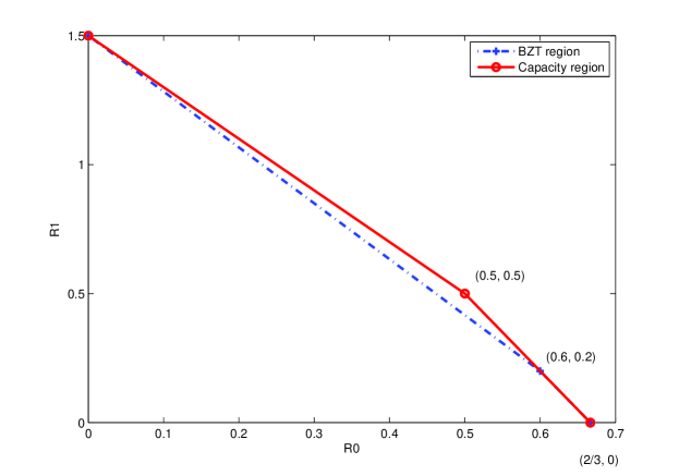
Figure 3: The BZT and the capacity regions for the channel in Figure 2.

Figure 3 plots the BZT region and the capacity region for the example channel. Both regions are specified by two line segments. The boundary of the BZT regions consists of the line segments: $(0,3/2)$ to $(0.6,0.2)$ and $(0.6,0.2)$ to $(2/3,0)$. The capacity region on the other hand is formed by the pair of line segments: $(0,3/2)$ to $(1/2,1/2)$ and $(1/2,1/2)$ to $(2/3,0)$. Note that the boundaries of the two regions coincide on the line segment joining $(0.6,0.2)$ to $(2/3,0)$.

Remarks:

1. Consider a 3-receiver Gaussian product multilevel broadcast channel, where

   $$Y_{21} =X_{1}+Z_{1},\;Y_{11}=Y_{21}+Z_{2},\;Y_{31}=Y_{11}+Z_{3},$$

   $$Y_{22} =X_{2}+Z_{4},\;Y_{32}=Y_{22}+Z_{5}.$$

   The noise power for $Z_{i}$ is $N_{i}$ for $i=1,2,\ldots,5$. We assume a total average power constraint $P$ on $X=(X_{1},X_{2})$.

   Using Gaussian signalling it can be easily shown that the BZT region is the set of all $(R_{0},R_{1})$ such that

   $$R_{0} \leq{\cal C}\left(\frac{\alpha P_{1}}{\bar{\alpha}P_{1}+N_{1}+N_{2}+N_{3}}\right)+{\cal C}\left(\frac{\beta(P-P_{1})}{\bar{\beta}(P-P_{1})+N_{4}+N_{5}}\right),$$ (12)

   $$R_{0} \leq{\cal C}\left(\frac{\alpha P_{1}}{\bar{\alpha}P_{1}+N_{1}}\right),$$

   $$R_{1} \leq{\cal C}\left(\frac{\bar{\alpha}P_{1}}{N_{1}+N_{2}}\right)+{\cal C}\left(\frac{\bar{\beta}(P-P_{1})}{N_{4}}\right),$$

   for some $0\leq P_{1}\leq P$, $0\leq\alpha,\beta\leq 1$.

   Now if we use Gaussian signaling to evaluate region (9), one obtains the achievable rate region consisting of the set of all $(R_{0},R_{1})$ such that

   $$R_{0} \leq{\cal C}\left(\frac{a_{1}P_{1}}{\bar{a}_{1}P_{1}+N_{1}+N_{2}+N_{3}}\right)+{\cal C}\left(\frac{a_{2}(P-P_{1})}{\bar{a}_{2}(P-P_{1})+N_{4}+N_{5}}\right),$$

   $$R_{0} \leq{\cal C}\left(\frac{(a_{1}+b_{1})P_{1}}{(1-a_{1}-b_{1})P_{1}+N_{1}}\right),$$

   $$R_{0}+R_{1} \leq{\cal C}\left(\frac{\bar{a}_{1}P_{1}}{N_{1}+N_{2}}\right)+{\cal C}\left(\frac{\bar{a}_{2}(P-P_{1})}{N_{4}}\right)+{\cal C}\left(\frac{a_{1}P_{1}}{\bar{a}_{1}P_{1}+N_{1}+N_{2}+N_{3}}\right)$$

   $$\quad+{\cal C}\left(\frac{a_{2}(P-P_{1})}{\bar{a}_{2}(P-P_{1})+N_{4}+N_{5}}\right),$$ (13)

   $$R_{0}+R_{1} \leq{\cal C}\left(\frac{((1-a_{1}-b_{1})P_{1}}{N_{1}+N_{2}}\right)+{\cal C}\left(\frac{(1-a_{2}-b_{2})(P-P_{1})}{N_{4}}\right)$$

   $$\quad+{\cal C}\left(\frac{(a_{1}+b_{1})P_{1}}{(1-a_{1}-b_{1})P_{1}+N_{1}}\right),$$

   for some $0\leq P_{1}\leq P$, $0\leq a_{1},a_{2},b_{1},b_{2},a_{1}+b_{1},a_{2}+b_{2}\leq 1$.

   Now consider the above regions with the parameters values: $P=1,N_{1}=0.4,N_{2}=N_{3}=0.1,N_{4}=0.5,N_{5}=0.1$. Fixing $R_{1}=0.5\log(0.49/0.3)$, we can show that the maximum achievable $R_{0}$ in the Gaussian BZT region is $0.5\log(2.0566...)$. On the other hand, using the parameter values $b_{1}=0.05,1-a_{1}=0.1725$, $1-a_{2}=0.5079$, and $P_{1}=0.5680$ for the region given by (13), the pair $(0.5\log(2.0603),0.5\log(0.49/0.3))$ is in the exterior of the region. Thus restricted to Gaussian signalling the BZT region (8) is strictly contained in region (9). However, we have not been able to prove that Gaussian signaling is optimal for either the BZT region or the capacity region.

2. The reader may ask why we did not consider the more general product channel

   $$X_{1} \to Y_{21}\to Y_{11}\to Y_{31},$$

   $$X_{2} \to Y_{12}\to Y_{32}\to Y_{22}.$$

   In fact we considered this more general class at first but were unable to show that the capacity region conditions reduce to the separated form

   $$R_{0} \leq I(V_{11};Y_{31})+I(V_{12};Y_{32}),$$

   $$R_{0} \leq I(V_{21};Y_{21})+I(V_{22};Y_{22}),$$

   $$R_{0}+R_{1} \leq I(V_{11};Y_{31})+I(V_{12};Y_{32})+I(X_{1};Y_{11}|V_{11})+I(X_{2};Y_{12}|V_{12}),$$

   $$R_{0}+R_{1} \leq I(V_{21};Y_{21})+I(V_{22};Y_{22})+I(X_{1};Y_{11}|V_{21})+I(X_{2};Y_{12}|V_{12}),$$

   for some $p(v_{11})p(v_{21}|v_{11})p(x_{1}|v_{21})p(v_{12})p(v_{22}|v_{12})p(x_{2}|v_{22})$.

V Bounds on Capacity of General 3-Receiver Broadcast Channel with Degraded Message Sets

In this section we extend the results in Section III to obtain inner and outer bounds on the capacity region of general 3-receiver broadcast channel with degraded message sets. We first consider the same 2 degraded message set scenario as in Section III but without the condition that $X\to Y_{1}\to Y_{3}$ form a degraded broadcast channel. We establish inner and outer bounds for this case and show that they are tight when the channel $X\to Y_{1}$ is less noisy than the channel $X\to Y_{3}$, which is a more general class than degraded broadcast channels [13]. We then extend our results to the case of 3 degraded message sets, where $M_{0}$ is to be sent to all receivers, $M_{1}$ is to be sent to receivers $Y_{1}$ and $Y_{2}$ and $M_{2}$ is to be sent only to receiver $Y_{1}$. A special case of this inner bound gives an inner bound to the capacity of the 2 degraded message set scenario where $M_{0}$ is to be sent to all receivers and $M_{1}$ is to be sent to receivers $Y_{1}$ and $Y_{2}$ only.

V-A Inner and Outer Bounds for 2 Degraded Message Sets

We use superposition coding, indirect decoding, and the Marton achievability scheme for the general 2-receiver broadcast channels [14] to establish the following inner bound.

Proposition 5

A rate pair $(R_{1},R_{2})$ is achievable in a general 3-receiver broadcast channel with 2 degraded message sets if it satisfies the following inequalities:

$$R_{0} \leq\min\{I(U_{2};Y_{2}),I(U_{3};Y_{3})\},$$

$$2R_{0} \leq I(U_{2};Y_{2})+I(U_{3};Y_{3})-I(U_{2};U_{3}|U_{1}),$$

$$R_{1} \leq\min\{I(X;Y_{1}|U_{2})+I(X;Y_{1}|U_{3}),I(X;Y_{1}|U_{1})\},$$ (14)

$$R_{0}+R_{1} \leq\min\{I(X;Y_{1}),I(U_{2};Y_{2})+I(X;Y_{1}|U_{2}),I(U_{3};Y_{3})+I(X;Y_{1}|U_{3})\},$$

$$2R_{0}+R_{1} \leq I(U_{2};Y_{2})+I(U_{3};Y_{3})+I(X;Y_{1}|U_{2},U_{3})-I(U_{2};U_{3}|U_{1}),$$

$$2R_{0}+2R_{1} \leq I(U_{2};Y_{2})+I(X;Y_{1}|U_{2})+I(U_{3};Y_{3})+I(X;Y_{1}|U_{3})-I(U_{2};U_{3}|U_{1}),$$

for some $p(u_{1},u_{2},u_{3},x)=p(u_{1})p(u_{2}|u_{1})p(x,u_{3}|u_{2})=p(u_{1})p(u_{3}|u_{1})p(x,u_{2}|u_{3})$ (or in other words, both $U_{1}\to U_{2}\to(U_{3},X)$ and $U_{1}\to U_{3}\to(U_{2},X)$ form Markov chains).

Proof:

The general idea of the proof is to represent $M_{0}$ by $U_{1}$, superimpose two independent pieces of information about $M_{1}$ to obtain $U_{2}$ and $U_{3}$, respectively, and then superimpose the remaining information about $M_{1}$ to obtain $X$. Receiver $Y_{1}$ decodes $U_{1},U_{2},U_{3},X$, receivers $Y_{2}$ and $Y_{3}$ find $M_{0}$ via indirect decoding of $U_{2}$ and $U_{3}$, respectively, as in Theorem 1. We now provide an outline of the proof

Code Generation: Let $R_{1}=S_{1}+S_{2}+S_{3}$, where the $S_{i}\geq 0$, $i=1,2,3$ and $T_{2}\geq S_{2}$, $T_{3}\geq S_{3}$. Fix a probability mass function of the required form, $p(u_{1},u_{2},u_{3},x)=p(u_{1})p(u_{2}|u_{1})p(x,u_{3}|u_{2})=p(u_{1})p(u_{3}|u_{1})p(x,u_{2}|u_{3})$.

Generate $2^{nR_{0}}$ sequences $U_{1}^{n}(m_{0})$, $m_{0}\in[1,2^{nR_{0}}]$ distributed uniformly at random over the set of typical $U_{1}^{n}$ sequences. For each $U_{1}^{n}(m_{0})$ generate $2^{nT_{2}}$ sequences $U_{2}^{n}(m_{0},t_{2})$, $t_{2}\in[1,2^{nT_{2}}]$ distributed uniformly at random from the set of conditionally typical $U_{2}^{n}$ sequences, and $2^{nT_{3}}$ sequences $U_{3}^{n}(m_{0},t_{3})$, $t_{3}\in[1,2^{nT_{3}}]$ distributed uniformly at random over the set of conditionally typical $U_{3}^{n}$ sequences. Randomly partition the $2^{nT_{2}}$ sequences $U_{2}^{n}(m_{0},t_{2})$ into $2^{nS_{2}}$ equal size bins and the $2^{nT_{3}}$ $U_{3}^{n}(m_{0},t_{3})$ sequences into $2^{nS_{3}}$ equal size bins. To ensure that each product bin contains a jointly typical pair $(U_{2}^{n}(m_{0},t_{2}),U_{3}^{n}(m_{0},t_{3}))$ with arbitrarily high probability, we require that (see  [15] for the proof)

$$S_{2}+S_{3}<T_{2}+T_{3}-I(U_{2};U_{3}|U_{1}).$$ (15)

Finally for each chosen jointly typical pair $(U_{2}^{n}(m_{0},t_{2}),U_{3}^{n}(m_{0},t_{3}))$ in each product bin $(s_{2},s_{3})$, generate $2^{nS_{1}}$ sequences of codewords $X^{n}(m_{0},s_{2},s_{3},s_{1})$, $s_{1}\in[1,2^{nS_{1}}]$ distributed uniformly at random over the set of conditionally typical $X^{n}$ sequences.

Encoding:

To send the message pair $(m_{0},m_{1})$, we express $m_{1}$ by the triple $(s_{1},s_{2},s_{3})$ and send the codeword $X^{n}(m_{0},s_{2},s_{3},s_{1})$.

Decoding:

1. Receiver $Y_{1}$ declares that $(m_{0},s_{2},s_{3},s_{1})$ is sent if it is the unique rate tuple such that $Y_{1}^{n}$ is jointly typical with $((U_{1}^{n}(m_{0}),U_{2}^{n}(m_{0},t_{2}),U_{3}^{n}(m_{0},t_{3}),X^{n}(m_{0},s_{2},s_{3},s_{1}))$, and $s_{2}$ is the product bin number of $U_{2}^{n}(m_{0},t_{2})$ and $s_{3}$ is the product bin number of $U_{2}^{n}(m_{0},t_{3})$. Assuming $(m_{0},s_{1},s_{2},s_{3})=(1,1,1,1)$ is sent, we partition the error event into the following events.

   1. Error event corresponding to $m_{0}\neq 1$ occurs with arbitrarily small probability provided

      $$R_{0}+S_{1}+S_{2}+S_{3}<I(X;Y_{1}).$$ (16)

   2. Error event corresponding to $m_{0}=1,s_{2}\neq 1,s_{3}\neq 1$ occurs with arbitrarily small probability provided

      $$S_{1}+S_{2}+S_{3}<I(X;Y_{1}|U_{1}).$$ (17)

   3. Error event corresponding to $m_{0}=1,s_{2}=1,s_{3}\neq 1$ occurs with arbitrarily small probability provided

      $$S_{1}+S_{3}<I(X;Y_{1}|U_{1},U_{2})=I(X;Y_{1}|U_{2}).$$ (18)

      The equality follows from the fact that $U_{1}\to U_{2}\to(U_{3},X)$ form a Markov Chain.

   4. Error event corresponding to $m_{0}=1,s_{2}\neq 1,s_{3}=1$ occurs with arbitrarily small probability provided

      $$S_{1}+S_{2}<I(X;Y_{1}|U_{1},U_{3})=I(X;Y_{1}|U_{3}).$$ (19)

      The above equality uses the fact that $U_{1}\to U_{3}\to(U_{2},X)$ forms a Markov chain.

   5. Error event corresponding to $m_{0}=1,s_{2}=1,s_{3}=1,s_{1}\neq 1$ occurs with arbitrarily small probability provided

      $$S_{1}<I(X;Y_{1}|U_{1},U_{2},U_{3})=I(X;Y_{1}|U_{2},U_{3}).$$ (20)

      Note that the equality here uses a weaker Markov structure $U_{1}\to(U_{2},U_{3})\to X$.

   Thus receiver $Y_{1}$ decodes $(m_{0},s_{2},s_{3},s_{1})$ with arbitrarily small probability of error provided equations (16)-(20) hold.

2. Receiver $Y_{2}$ decodes $m_{0}$ via list decoding of $U_{2}^{n}(m_{0},t_{2})$ (as in Theorem 1). This can be achieved with arbitrarily small probability of error provided

   $$R_{0}+T_{2}<I(U_{2};Y_{2}).$$ (21)

3. Receiver $Y_{3}$ decodes $m_{0}$ via list decoding of $U_{2}^{n}(m_{0},t_{3})$ (as in Theorem 1). This can be achieved with arbitrarily small probability of error provided

   $$R_{0}+T_{3}<I(U_{3};Y_{3}).$$ (22)

Combining equations (15)-(22) and using the Fourier-Motzkin procedure [16] to eliminate $T_{2},T_{3},S_{1},S_{2}$, and $S_{3}$, we obtain the inequalities in (5). The details are given in Appendix B. ∎

Remarks:

1. The above achievability scheme can be adapted to any joint distribution $p(u_{1},u_{2},u_{3},x)$. However by letting $\tilde{U}_{2}=(U_{2},U_{1})$ and letting $\tilde{U}_{3}=(U_{3},U_{1})$ we observe that the region remains unchanged. Hence, without loss of generality we assume the structure of the auxiliary random variables as described in the proposition. It is also interesting to note that the auxiliary random variables in the outer bound described in the next subsection also possess the same structure.

2. An interesting choice of the auxiliary random variables is to set $U_{2}$ or $U_{3}$ equal to $U_{1}$ (i.e., only one of the the receivers tries to indirectly decode $M_{0}$), say let $U_{3}=U_{1}$. This reduces the inequalities  5 (after removing the redundant ones) to:

   $$R_{0} \leq\min\{I(U_{2};Y_{2}),I(U_{1};Y_{3})\},$$

   $$R_{1} \leq I(X;Y_{1}|U_{1}),$$ (23)

   $$R_{0}+R_{1} \leq\min\{I(X;Y_{1}),I(U_{2};Y_{2})+I(X;Y_{1}|U_{2}),I(U_{1};Y_{3})+I(X;Y_{1}|U_{1})\},$$

   where $U_{1}\to U_{2}\to X$ form a Markov chain.

   This region includes the capacity region of the multilevel case in Theorem 1. It is easy to verify that for any $U_{1}\to U_{2}\to X$ that form a Markov chain, the corner points of the region in Theorem 1 satisfy the above inequalities (and this suffices by convexity).

We now establish the following outer bound

Proposition 6

Any achievable rate pair $(R_{0},R_{1})$ for the general 3-receiver broadcast channel with 2 degraded message sets must satisfy the conditions:

$$R_{0} \leq\min\{I(U_{1};Y_{1}),I(U_{2};Y_{2})-I(U_{2};Y_{1}|U_{1}),I(U_{3};Y_{3})-I(U_{3};Y_{1}|U_{1})\},$$

$$R_{1} \leq I(X;Y_{1}|U_{1}).$$

for some $p(u_{1},u_{2},u_{3},x)=p(u_{1})p(u_{2}|u_{1})p(x,u_{3}|u_{2})=p(u_{1})p(u_{3}|u_{1})p(x,u_{2}|u_{3})$, i.e., the same structure of the auxiliary random variables as in Lemma 5. Further one can restrict the cardinalities of $U_{1},U_{2},U_{3}$ to: $\|\mathcal{U}_{1}\|\leq\|\mathcal{X}\|+6$, $\|\mathcal{U}_{2}\|\leq(\|\mathcal{X}\|+1)(\|\mathcal{X}\|+6)$, and $\|\mathcal{U}_{3}\|\leq(\|\mathcal{X}\|+1)(\|\mathcal{X}\|+6)$.

Proof:

The proof follows largely standard arguments. The auxiliary random variables are identified as $U_{1i}=(M_{0},Y_{1}^{i-1})$, $U_{2i}=(U_{1i},Y_{2~{}i+1}^{~{}n})$, $U_{3i}=(U_{1i},Y_{3~{}i+1}^{~{}n})$. With this identification inequalities $R_{0}\leq I(U_{1};Y_{1})$ and $R_{1}\leq I(X;Y_{1}|U_{1})$ is immediate. The other two inequalities also follow from standard arguments and is briefly outlined here.

$$nR_{0} \leq n\lambda_{n}+\sum_{i}I(M_{0};Y_{3i}|Y_{3~{}i+1}^{~{}n})$$

$$\leq n\lambda_{n}+\sum_{i}I(M_{0},Y_{3~{}i+1}^{~{}n},Y_{1}^{i-1};Y_{3i})-I(Y_{1}^{i-1};Y_{3i}|M_{0},Y_{3~{}i+1}^{~{}n})$$

$$\stackrel{{\scriptstyle(a)}}{{=}}n\lambda_{n}+\sum_{i}I(M_{0},Y_{3~{}i+1}^{~{}n},Y_{1}^{i-1};Y_{3i})-I(Y_{3~{}i+1}^{~{}n};Y_{1i}|M_{0},Y_{1}^{i-1})$$

$$=n\lambda_{n}+\sum_{i}I(U_{3i};Y_{3i})-I(U_{3i};Y_{1i}|U_{1i}),$$

where $(a)$ uses the Csiszár sum equality.

The cardinality bounds are established using a similar argument as in III-C. To create a set of new auxiliary random variables with the bounds of Proposition 6, we first replace $U_{2}$ by $(U_{2},U_{1})$ and $U_{3}$ by $(U_{3},U_{1})$. It is easy to see from the Markov chain relationships $U_{1}\to U_{2}\to(U_{3},X)$ and $U_{1}\to U_{3}\to(U_{2},X)$ that the following region is same as the that of Proposition 6.

$$R_{0} \leq\min\{I(U_{1};Y_{1}),I(U_{1},U_{2};Y_{2})+I(X;Y_{1}|U_{1},U_{2})-I(X:Y_{1}|U_{1}),$$

$$\qquad I(U_{1},U_{3};Y_{3})+I(X;Y_{1}|U_{1},U_{3})-I(X:Y_{1}|U_{1})\},$$ (24)

$$R_{1} \leq I(X;Y_{1}|U_{1}).$$

Then using standard arguments one can replace $U_{1}$ by $U_{1}^{*}$ satisfying $\|\mathcal{U}_{1}^{*}\|\leq\|\mathcal{X}\|+6$, such that the distribution of $X$ and $H(Y_{1}|U_{1})$, $H(Y_{1}|U_{1},U_{2})$, $H(Y_{1}|U_{1},U_{3})$, $H(Y_{2}|U_{1})$, $H(Y_{2}|U_{1},U_{2})$, $H(Y_{3}|U_{1})$, and $H(Y_{3}|U_{1},U_{3})$ are preserved. Now for each $U_{1}^{*}=u_{1}$ one can find $U_{2}^{*}(u_{1})$ with cardinality less than $\|\mathcal{X}\|+1$ each such that the distribution of $X$ conditioned on $U_{1}^{*}=u_{1}$, $H(Y_{1}|U_{1}^{*}=u_{1},U_{2})$, and $H(Y_{2}|U_{1}^{*}=u_{1},U_{2})$ are preserved. Similarly one can find for each $U_{1}^{*}=u_{1}$, a random variable $U_{3}^{*}(u_{1})$ with cardinality less than $\|\mathcal{X}\|+1$ each such that the distribution of $X$ conditioned on $U_{1}^{*}=u_{1}$, $H(Y_{1}|U_{1}^{*}=u_{1},U_{3})$, and $H(Y_{3}|U_{1}^{*}=u_{1},U_{3})$ are preserved. This yields random variables $U_{1}^{*},U_{2}^{*},U_{3}^{*}$ that preserve the region in (24). (Note that as the distribution of $X$ conditioned on $U_{1}=u_{1}$ is preserved by both $U_{2}^{*}(u_{1})$ and $U_{3}^{*}(u_{1})$, it is possible to get a consistent triple of random variables $U_{1}^{*},U_{2}^{*},U_{3}^{*}$.) Finally setting $\tilde{U}_{1}=U_{1}^{*}$, $\tilde{U}_{2}=(U_{1}^{*},U_{2}^{*})$ and $\tilde{U}_{3}=(U_{1}^{*},U_{3}^{*})$ gives the desired bounds on cardinality as well as the desired Markov relations. ∎

Remarks:

1. The above outer bound appears to be very different from the inner bound of Proposition 5. However, by taking appropriate sums of the inequalities defining the region of Proposition 6, we arrive at the conditions

   $$R_{0} \leq\min\{I(U_{2};Y_{2})-I(U_{2};Y_{1}|U_{1}),I(U_{3};Y_{3})-I(U_{3};Y_{1}|U_{1})),$$

   $$R_{1} \leq I(X;Y_{1}|U_{1}),$$

   $$R_{0}+R_{1} \leq\min\{I(X;Y_{1}),I(U_{2};Y_{2})+I(X;Y_{1}|U_{2}),I(U_{3};Y_{3})+I(X;Y_{1}|U_{3})\},$$

   $$2R_{0}+R_{1} \leq I(U_{2};Y_{2})+I(U_{3};Y_{3})+I(X;Y_{1}|U_{2},U_{3})-I(U_{2};U_{3}|U_{1})+I(U_{2};U_{3}|Y_{1},U_{1}).$$

   These conditions include some redundant ones, but are closer in structure to the inequalities defining the inner bound of Proposition 5.

2. The outer bound in Proposition 6 reduces to the capacity region for the multilevel case in Theorem 1. To see this observe that when $X\to Y_{1}\to Y_{3}$ form a Markov chain,

   $$R_{0}\leq I(U_{3};Y_{3})-I(U_{3};Y_{1}|U_{1})\leq I(U_{3};Y_{3})-I(U_{3};Y_{3}|U_{1})=I(U_{1};Y_{3}).$$ (25)

   Further from $R_{1}\leq I(X;Y_{1}|U_{1})$, we have $R_{0}+R_{1}\leq I(U_{1};Y_{3})+I(X;Y_{1}|U_{1})$. Thus the outer bound is contained in the achievable region of Theorem 1, i.e.,

   $$R_{0} \leq\min\{I(U_{1};Y_{3}),I(U_{2};Y_{2})\},$$ (26)

   $$R_{0}+R_{1} \leq\{I(U_{1};Y_{3})+I(X;Y_{1}|U_{1}),I(U_{2};Y_{2})+I(X;Y_{1}|U_{2})\}.$$

3. The inner and outer bounds match if $Y_{1}$ is less noisy than $Y_{3}$ [13], that is if $I(U;Y_{3})\leq I(U;Y_{1})$ for all $p(u)p(x|u)$. As shown in  [13], this condition is more general than degradedness. As such, it defines a larger class than multilevel broadcast channels.

   Proposition 7

   The capacity region for the 3-receiver broadcast channel with 2 degraded message sets when $Y_{1}$ is a less noisy receiver than $Y_{3}$ is given by the set of rate pairs $(R_{0},R_{1})$ such that

   $$R_{0} \leq\min\{I(U_{1};Y_{3}),I(U_{2};Y_{2})\},$$ (27)

   $$R_{0}+R_{1} \leq\min\{I(U_{1};Y_{3})+I(X;Y_{1}|U_{1}),I(U_{2};Y_{2})+I(X;Y_{1}|U_{2})\},$$

   for some $p(u_{1})p(u_{2}|u_{1})p(x|u_{2})$.

   From the definition of less noisy receivers [13] we have $I(U_{3};Y_{3}|U_{1}=u_{1})\leq I(U_{3};Y_{1}|U_{1}=u_{1})$ for every choice of $u_{1}$ and thus $I(U_{3};Y_{3}|U_{1})\leq I(U_{3};Y_{1}|U_{1})$ for every $p(u_{1})p(u_{3}|u_{1})p(x|u_{3})$. Using (25) it follows that the general outer bound is contained in (27). The corner point of (27) (under the less noisy assumption) is contained in the region given by (23) and thus achievable by setting $U_{3}=U_{1}$ in the region of Proposition 5.

V-B Inner Bound for 3 Degraded Message Sets

In this section we establish an inner bound to the capacity region of the broadcast channel with 3 degraded message sets where $M_{0}$ is to be sent to all three receivers, $M_{1}$ is to be sent only to $Y_{1}$ and $Y_{2}$, and $M_{2}$ is to be sent only to $Y_{1}$. We then specialize the result to the case of 2 degraded message sets scenario, where $M_{0}$ is to be sent to all receivers and $M_{1}$ is to be sent to $Y_{1}$ and $Y_{2}$ and establish optimality for two classes of channels.

The inner bound we establish is closely related to that of Proposition 5. To explain the connection, consider a 3-receiver broadcast channel scenario where message $M_{0}$ is to be sent to all three receivers, message $M_{12}$ is to be sent to receivers $Y_{1}$ and $Y_{2}$, message $M_{13}$ is to be sent to receivers $Y_{1}$ and $Y_{3}$, and message $M_{11}$ is to be sent only to receiver $Y_{1}$. An inner bound to the capacity region for this scenario that uses superposition coding and Marton’s coding scheme would be to represent $M_{0}$ by an auxiliary random variable $U_{1}$, $(M_{0},M_{12})$ by an auxiliary random variable $U_{2}$, $(M_{0},M_{13})$ by $U_{3}$, and $(M_{0},M_{12}.M_{13},M_{11})$ by $X$, where $U_{1}\to U_{2}\to(U_{3},X)$ and $U_{1}\to U_{3}\to(U_{2},X)$ form Markov chains.

The inner bound of Proposition 5 follows from the above scenario by relaxing the conditions that $Y_{2}$ needs to decode $M_{12}$ and $Y_{3}$ needs to decode $M_{13}$ and considering both messages as parts of the private message to receiver $Y_{1}$. However, instead of eliminating the auxiliary random variables $U_{2}$ and $U_{3}$ completely (as in the BZT region, which is a straightforward extension of the Körner-Marton scheme), we keep them and have receivers $Y_{2}$ and $Y_{3}$ use the new technique of indirect decoding to find $M_{0}$ through $U_{2}$ and $U_{3}$, respectively. As we have shown in Section IV, having these random variables $U_{2}$ and $U_{3}$ can strictly improve the achievability region of the 2-message sets scenario.

Now consider the 3 degraded message set scenario. We relax the condition in the above scenario that $Y_{3}$ needs to decode $M_{13}$. Recall the proof of Proposition 5. We let $R_{1}=S_{2}$, $R_{2}=S_{3}+S_{1}$ and represent $M_{0}$ by $U_{1}$, $(M_{0},M_{1})$ by $U_{2}$, $(M_{0},S_{3})$ by $U_{3}$, and $(M_{0},M_{1},M_{2})$ by $X$. Receiver $Y_{1}$ finds $(M_{0},M_{1},M_{2})$ by decoding $U_{1},U_{2},U_{3},X$; receiver $Y_{2}$ finds $(M_{0},M_{1})$ by decoding $U_{1},U_{2}$; and receiver $Y_{3}$ finds $M_{0}$ by indirectly decoding $U_{1}$ through $U_{3}$. We obtain the following conditions for achievability of any rate tuple $(R_{0},R_{1},S_{3},S_{1})$ by replacing $S_{2}$ by $R_{1}$ in conditions  (15)-(22) and adding the condition $T_{2}<I(U_{2};Y_{2}|U_{1})$ (to enable $Y_{2}$ to completely decode $U_{2}$).

$$R_{1} \leq T_{2},$$

$$S_{3} \leq T_{3},$$

$$R_{1}+S_{3} \leq T_{2}+T_{3}-I(U_{2};U_{3}|U_{1}),$$

$$R_{0}+S_{1}+R_{1}+S_{3} \leq I(X;Y_{1}),$$

$$S_{1}+S_{3} \leq I(X;Y_{1}|U_{1},U_{2})=I(X;Y_{1}|U_{2}),$$

$$S_{1}+R_{1} \leq I(X;Y_{1}|U_{1},U_{3})=I(X;Y_{1}|U_{3}),$$ (28)

$$S_{1}+R_{1}+S_{3} \leq I(X;Y_{1}|U_{1}),$$

$$S_{1} \leq I(X;Y_{1}|U_{1},U_{2},U_{3})=I(X;Y_{1}|U_{2},U_{3}),$$

$$R_{0}+T_{2} \leq I(U_{1},U_{2};Y_{2})=I(U_{2};Y_{2}),$$

$$T_{2} \leq I(U_{2};Y_{2}|U_{1}),$$

$$R_{0}+T_{3} \leq I(U_{1},U_{3};Y_{3})=I(U_{3};Y_{3}),$$

for some $p(u_{1},u_{2},u_{3},x)=p(u_{1})p(u_{2}|u_{1})p(x,u_{3}|u_{2})=p(u_{1})p(u_{3}|u_{1})p(x,u_{2}|u_{3})$.

Performing Fourier-Motzkin procedure to eliminate the variables $S_{1},S_{3},T_{2}$ and $T_{3}$ yields the following achievable region.

Theorem 2

A rate triple $(R_{0},R_{1},R_{2})$ is achievable in a general 3-receiver broadcast channel with 3 degraded message sets if it satisfies the conditions:

$$R_{0} \leq I(U_{3};Y_{3})$$

$$R_{1} \leq\min\{I(U_{2};Y_{2}|U_{1}),I(X;Y_{1}|U_{3})\},$$

$$R_{2} \leq I(X;Y_{1}|U_{2})$$

$$R_{0}+R_{1} \leq\min\{I(U_{2};Y_{2}),I(U_{2};Y_{2}|U_{1})+I(U_{3};Y_{3})-I(U_{2};U_{3}|U_{1})\},$$

$$2R_{0}+R_{1} \leq I(U_{2};Y_{2})+I(U_{3};Y_{3})-I(U_{2};U_{3}|U_{1}),$$

$$R_{0}+R_{2} \leq I(U_{3};Y_{3})+I(X;Y_{1}|U_{2},U_{3})$$

$$R_{1}+R_{2} \leq I(X;Y_{1}|U_{1}),$$

$$R_{0}+R_{1}+R_{2} \leq\min\{I(X;Y_{1}),I(U_{3};Y_{3})+I(X;Y_{1}|U_{3}),$$

$$\qquad I(U_{2};Y_{2}|U_{1})+I(U_{3};Y_{3})+I(X;Y_{1}|U_{2},U_{3})-I(U_{2};U_{3}|U_{1})\},$$ (29)

$$2R_{0}+R_{1}+R_{2} \leq I(U_{2};Y_{2})+I(U_{3};Y_{3})+I(X;Y_{1}|U_{2},U_{3})-I(U_{2};U_{3}|U_{1}),$$

$$R_{0}+2R_{1}+R_{2} \leq I(U_{2};Y_{2}|U_{1})+I(U_{3};Y_{3})+I(X;Y_{1}|U_{3})-I(U_{2};U_{3}|U_{1}),$$

$$2R_{0}+2R_{1}+R_{2} \leq I(U_{2};Y_{2})+I(U_{3};Y_{3})+I(X;Y_{1}|U_{3})-I(U_{2};U_{3}|U_{1}).$$

for some $p(u_{1},u_{2},u_{3},x)=p(u_{1})p(u_{2}|u_{1})p(x,u_{3}|u_{2})=p(u_{1})p(u_{3}|u_{1})p(x,u_{2}|u_{3})$ (i.e., as before both $U_{1}$ $\to U_{2}$ $\to(U_{3},X)$ and $U_{1}\to U_{3}\to(U_{2},X)$ form Markov chains).

Remark: The region of Theorem 2 reduces to the inner bound of Proposition 5 by setting $R_{1}=0$. The equivalence between the two descriptions is proved in Appendix C.

We now consider a 2 degraded message set scenario where $M_{0}$ is to be sent to all receivers and $M_{1}$ is to be sent to receivers $Y_{1}$ and $Y_{2}$. The following inner bound follows from Theorem 2 by setting $R_{2}=0$.

Corollary 1

A rate pair $(R_{0},R_{1})$ is achievable in a 3-receiver broadcast channel with 2 degraded message sets, where $M_{0}$ is to be decoded by all three receivers and $M_{1}$ is to be decoded only by $Y_{1}$ and $Y_{2}$ if it satisfies the following conditions:

$$R_{0} \leq I(U;Y_{3}),$$

$$R_{1} \leq\min\{I(X;Y_{2}|U),I(X;Y_{1}|U)\},$$ (30)

$$R_{0}+R_{1} \leq\min\{I(X;Y_{2}),I(X;Y_{1})\},$$

for some $p(u)p(x|u)$.

Remarks:

1. Region (30) coincides with the straightforward extension of the Körner-Marton 2-receiver region.

2. By setting $R_{2}=0$, $U_{2}=X$, and $U_{3}=U_{1}=U$ the region in Theorem 2 reduces to (30). Thus region in (30) is contained in region (29).

3. It may seem that the region obtained by setting $R_{2}=0$ in (29) is larger than region (30), but they are in fact equal. variables, we see that Therefore, there is no need to introduce $U_{3}$. To prove this, observe that

   $$R_{0}+R_{1} \leq I(U_{2};Y_{2}|U_{1})+I(U_{3};Y_{3})-I(U_{2};U_{3}|U_{1})$$

   $$=I(U_{3};Y_{3})+I(U_{3};Y_{2}|U_{1})+I(U_{2};Y_{2}|U_{3})-I(U_{3};Y_{2}|U_{2})-I(U_{3};U_{2}|U_{1})$$

   $$=I(U_{3};Y_{3})+I(U_{2};Y_{2}|U_{3})-I(U_{3};U_{2}|Y_{2},U_{1})$$

   $$\leq I(U_{3};Y_{3})+I(X;Y_{2}|U_{3}).$$

   Thus the rate pairs must satisfy the following inequalities

   $$R_{0} \leq I(U_{3};Y_{3}),$$

   $$R_{0}+R_{1} \leq\min\{I(U_{3};Y_{3})+I(X;Y_{2}|U_{3}),I(U_{3};Y_{3})+I(X;Y_{1}|U_{3})\},$$ (31)

   $$R_{0}+R_{1} \leq\min\{I(X;Y_{2}),I(X;Y_{1})\}.$$

   Clearly this is contained inside region (30) and hence region (29) reduces to the one in Corollary 1 when $R_{2}=0$.

4. Inner bound (30) is optimal for the following two special classes of broadcast channels.

   Proposition 8

   Achievable region (30) is tight for deterministic 3-receiver broadcast channels.

   It is straightforward to show that the set of rate pairs $(R_{0},R_{1})$ such that

   $$R_{0} \leq\min\{H(Y_{1}),H(Y_{2}),H(Y_{3})\},$$

   $$R_{0}+R_{1} \leq\min\{H(Y_{2}),H(Y_{1})\},$$

   for some $p(x)$ constitutes an outer bound on the capacity region. To show achievability, we need only consider the three choices for $U$: (i) $U=Y_{3}$, and (ii) $U=X$, and (iii) $U=\emptyset$.

   Proposition 9

   Achievable region (30) is optimal when $Y_{1}$ is a less noisy receiver than $Y_{3}$ and $Y_{2}$ is a less noisy receiver than $Y_{3}$.

   Note that this result generalizes Theroem 3.2 in [4] where the authors assume the receivers are $Y_{2}$ and $Y_{1}$ are degraded versions of $Y_{3}$. To show optimality, we set $U_{i}=(M_{0},Y_{3}^{i-1})$ and thus the only non-trivial inequality in the converse is $R_{1}\leq\min\{I(X;Y_{1}|U),I(X;Y_{2}|U)\}$. To see this observe that

   $$nR_{1} \leq\sum_{i}I(M_{1};Y_{1i}|M_{0},Y_{1~{}i+1}^{n})$$

   $$\leq\sum_{i}I(M_{1};Y_{1i}|M_{0},Y_{1~{}i+1}^{n},Y_{3}^{i-1})+\sum_{i}I(Y_{3}^{i-1};Y_{1i}|M_{0},Y_{1~{}i+1}^{n}))$$

   $$\stackrel{{\scriptstyle(a)}}{{=}}\sum_{i}I(M_{1},Y_{1~{}i+1}^{n};Y_{1i}|M_{0},Y_{3}^{i-1})-\sum_{i}I(Y_{1~{}i+1}^{n};Y_{1i}|M_{0},Y_{3}^{i-1})+\sum_{i}I(Y_{1~{}i+1}^{n};Y_{3i}|M_{0},Y_{3}^{i-1})$$

   $$\stackrel{{\scriptstyle(b)}}{{\leq}}\sum_{i}I(X_{i};Y_{1i}|M_{0},Y_{3}^{i-1}),$$

   where $(a)$ uses the Csiszár sum equality and $(b)$ uses the assumption that $Y_{1}$ is a less noisy than $Y_{3}$, which implies that $I(Y_{1~{}i+1}^{n};Y_{3i}|M_{0},Y_{3}^{i-1})\leq I(Y_{1~{}i+1}^{n};Y_{1i}|M_{0},Y_{3}^{i-1})$. The bound $R_{1}\leq I(X;Y_{2}|U)$ can be proved similarly.

V-C Inner Bounds for $k$-receiver Broadcast Channels

The inner bounds discussed in previous subsections suggest the following extension to general $k$-receiver broadcast channel scenarios with given message requirements. To illustrate our procedure we shall use the running example of a 3-receiver broadcast channel with 3 messages to receiver subsets: $\{1\}$, $\{1,2\}$, and $\{2,3\}$.

To obtain an inner bound to capacity for a given message requirement, we first consider all nonempty receiver subsets. Let $\mathcal{S}_{D}$ be the collection of subsets specified by the message requirements. For each $A\in\mathcal{S}_{D}$, we introduce an auxiliary random variable for every $B\supset A$. Thus in our example, $\mathcal{S}_{D}=\left\{\{1\},\{2,3\},\{1,2\}\right\}$, and five auxiliary random variables are introduced corresponding to the subsets: $\{1,2,3\}$, $\{1,2\}$, $\{1,3\}$, $\{2,3\}$, and $\{1\}$. Let $\mathcal{S}_{I}$ denote the receiver subsets for which auxiliary random variables are introduced but are not in $\mathcal{S}_{D}$. In the example, $\mathcal{S}_{I}=\left\{\{1,3\},\{1,2,3\}\right\}$.

The receiver subsets with auxiliary random variables assigned to them are classified into levels based on their cardinality with the lowest level subsets having the largest cardinality. There is a Markov structure between the variables as follows: if $U_{B}$ represents the auxiliary random variable corresponding to the subset $B$ and $U_{A}$ represents the auxiliary random variable corresponding to the subset $A\subset B$, then one can set $U_{A}=(U_{B},\tilde{U}_{A})$. Thus an auxiliary random variable $U_{A}$ corresponding to a subset $A$ should contain all auxiliary random variables corresponding to the subsets $B\supset A$. For the running example, Level 1 contains the subset $\{1,2,3\}$, Level 2 contains the subsets $\{1,2\}$, $\{1,3\}$, and $\{2,3\}$, and Level 3 contains the subset $\{1\}$. The Markov relationships between these auxiliary random variables are defined by:

$$U_{12} =(U_{123},\tilde{U}_{12}),~{}U_{13}=(U_{123},\tilde{U}_{13}),~{}U_{23}=(U_{123},\tilde{U}_{23}),$$

$$U_{1} =\{U_{12},U_{13},\tilde{U}_{1}\}.$$

Code generation proceeds one level at a time beginning with the lowest level followed by the second lowest level, and so on. The codebooks corresponding to auxiliary random variables at each level are randomly generated conditioned on codewords at the lower level according to the Markov structure of the auxiliary random variables. Random binning is performed at each level to find jointly typical codewords to represent message products.

Decoding is performed at receiver $i$ as follows: let $T_{i}$ represent the collection of receiver subsets that contains $i$ for which auxiliary random variables are introduced. A subset $A\in T_{i}$ is said to be minimal if there is no $B\in T_{i}$ such that $B\subset A$. Let $\mathcal{T}^{\rm min}_{i}$ be the collection of minimal subsets in $T_{i}$. For the example we obtain

$$T_{1} =\left\{\{1,2,3\},\{1,2\},\{1,3\},\{1\}\right\}\text{ and }\mathcal{T}^{\rm min}_{1}=\{1\},$$

$$T_{2} =\left\{\{1,2,3\},\{1,2\},\{2,3\}\right\}\text{ and }\mathcal{T}^{\rm min}_{2}=\left\{\{1,2\},\{2,3\}\right\},$$

$$T_{3} =\left\{1,2,3\},\{1,3\},\{2,3\}\right\}\text{ and }\mathcal{T}^{\rm min}_{3}=\left\{\{1,3\},\{2,3\}\right\}.$$

By the Markov structure defined above, it is clear that all the messages for receiver $i$ are represented by the auxiliary random variables $\mathcal{U}^{\rm min}_{i}$, which correspond to the elements of $\mathcal{T}^{min}_{i}$. The auxiliary random variables in $\mathcal{U}^{min}_{i}\cap\mathcal{S}_{D}$ represent private messages for receiver $i$, while those in $\mathcal{U}^{min}_{i}\cap\mathcal{S}_{D}^{c}$ contain only parts of private messages. Receiver $i$ uses indirect decoding to find the private messages encoded into cloud centers by using the satellite codewords represented by the auxiliary random variables in $\mathcal{U}^{min}_{i}$.

In our running example, receiver $3$ indirectly decodes $U_{23}$ using the pair $(U_{13},U_{23})$. That is, the rate constraints are such that receiver $3$ may not be able to uniquely decode $U_{13}$ but is able to decode the correct $U_{23}$. However, receivers $Y_{2}$ and $Y_{1}$ should be able to correctly decode $(U_{12},U_{23})$ and $U_{1}$, respectively, and hence these receivers impose the usual (direct) decoding constraints on the rates. In general, when $\mathcal{U}^{min}_{i}\cap\mathcal{S}_{I}=\emptyset$, indirect decoding is not needed as in the Examples below, where as in Proposition 5 indirect decoding is needed.

The following two examples show that the above procedure yields the best known inner bounds for special classes of broadcast channels.

Example 1: 2-receiver broadcast channel where $M_{1}$ is to be decoded by receiver $Y_{1}$ and $M_{2}$ is to be decoded by $Y_{2}$. We generate 3 auxiliary random variables corresponding to the three non-empty subsets of $\{1,2\}$: $W$ for $\{1,2\}$, $U$ for $\{1\}$ and $V$ for $\{2\}$. Setting $\tilde{U}=(U,W)$ and $\tilde{V}=(V,W)$ represents the Markov structure among the variables. Observe that the auxiliary random variables are exactly as in Marton’s coding scheme and so is the code generation we outlined earlier.

Example 2: $k$-receiver broadcast channel with 2 degraded message sets, where $M_{0}$ is to be decoded by receivers $\{1,\ldots,k\}$ and $M_{1}$ is to be decoded by $\{1,\ldots,k-1\}$. The only subsets that we would assign auxiliary random variables to here are $\{1,\ldots,k\}$ and $\{1,\ldots,k-1\}$. We thus introduce the auxiliary random variable $U_{1}$ for $\{1,\ldots,k\}$ and $U_{2}$ for $\{1,\ldots,k-1\}$. The region is then be given by

$$R_{0} \leq I(U_{1};Y_{k}),$$

$$R_{0}+R_{1} \leq I(U_{2};Y_{i}),~{}\text{for}~{}i=1,\ldots,k-1,$$

$$R_{1} \leq I(U_{2};Y_{i}|U_{1})~{}\text{for}~{}i=1,\ldots,k-1,$$

where $U_{1}\to U_{2}\to X\to\{Y_{1},\ldots,Y_{l}\}$ form a Markov chain. Clearly in this case it is optimal to set $U_{2}=X$, which reduces the region to the straightforward extension of the Körner-Marton scheme.

Remark: Our procedure can result in an explosion in the number of auxiliary random variables introduced even in simple scenarios. However, as we have shown in Section IV, indirect decoding may be needed to achieve the capacity region for some classes of channels. Thus the introduction of such a large number of auxiliary random variables may indeed be necessary in general.

VI Conclusion

Recent results and conjectures on the capacity of $(k>2)$-receiver broadcast channels with degraded message sets  [6, 4, 5] have lent support to the general belief that the straightforward extension of the Körner-Marton region for the 2-receiver case is optimal. This paper shows that this is not the case. We show that the capacity region of the 3-receiver broadcast channels with 2 degraded message sets can be strictly larger than the straightforward extension of the Körner-Marton region. The achievability proof uses the new idea of indirect decoding whereby a receiver decodes a cloud center indirectly through joint typicality with a satellite codeword. Using this idea, we devise new inner bounds to the capacity of the general 3-receiver broadcast channel with 2 and 3 degraded message sets and show optimality in some cases. The structure of the auxiliary random variables in the inner bounds can be naturally extended to more than 3 receivers. The bounds also provide some insight into how the Marton achievable rate region may be extended to more than 2 receivers.

The results in this paper suggest that the capacity of the $k>2$-receiver broadcast channels with degraded message sets is as at least as hard to find as the capacity of the general 2-receiver broadcast channel with common and private message. However, it would be interesting to explore the optimality of our new inner bounds for classes where capacity is known for the general 2-receiver case, such as deterministic and vector Gaussian broadcast channels. It would also be interesting to investigate applications of indirect decoding to other problems, for example, $3$-receiver broadcast channels with confidential message sets [11].

Acknoledgement

The authors wish to thank Young-Han Kim for valuable suggestions that has improved the presentation of this paper.

Appendix A Proof of Propositions 1, 2, 3, and 4

To prove Propositions 1, 2, note that it is straightforward to show that each simplified characterization is contained in the original region as the characterizations are obtained by using the channels independently. So we only prove the other non-trivial direction.

Proof of Proposition 1:

We prove that for the product broadcast channel given by (IV) the BZT region (3) reduces to the expression (8).

Consider the first term (8a) in the BZT region

$$R_{0}\leq I(U;Y_{3}) =I(U;Y_{31},Y_{32})$$

$$=I(U;Y_{31})+I(U;Y_{32}|Y_{31})$$

$$\leq I(U;Y_{31})+I(U,Y_{31};Y_{32})$$

$$\leq I(U;Y_{31})+I(U,Y_{11};Y_{32}).$$

Now set $V_{1}=U$ and $V_{2}=(U,Y_{11})$. Thus the above inequality becomes

$$R_{0}\leq I(V_{1};Y_{31})+I(V_{2};Y_{32}).$$

The second term (8b) in the BZT region is simply given by

$$R_{0}\leq I(V_{1};Y_{21}).$$

Finally, consider the last term (8c)

$$R_{1}\leq I(X;Y|U) =I(X_{1},X_{2};Y_{11},Y_{12}|U)$$

$$=H(Y_{11},Y_{12}|U)-H(Y_{11},Y_{12}|X_{1},X_{2},U)$$

$$=H(Y_{11}|U)+H(Y_{12}|U,Y_{11})-H(Y_{11}|X_{1},U)-H(Y_{12}|X_{2},U)$$

$$=I(X_{1};Y_{11}|U)+H(Y_{12}|U,Y_{11})-H(Y_{12}|X_{2},U,Y_{11})$$

$$=I(X_{1};Y_{11}|V_{1})+I(X_{2};Y_{12}|V_{2}).$$

The fact that $p(v_{1})p(v_{2})p(x_{1}|v_{1})p(x_{2}|v_{2})$ suffices follows from the structure of the mutual information terms.

Proof of Proposition 2:

We prove that for the product broadcast channel (IV) the capacity region given by Theorem 1 reduces to the expression (9).

Consider the first term (9a) in the capacity region

$$R_{0}\leq I(U_{1};Y_{3}) =I(U_{1};Y_{31},Y_{32})$$

$$=I(U_{1};Y_{31})+I(U_{1};Y_{32}|Y_{31})$$

$$\leq I(U_{1};Y_{31})+I(U_{1},Y_{31};Y_{32})$$

$$\leq I(U_{1};Y_{31})+I(U_{1},Y_{11};Y_{32}).$$

Now set $V_{11}=U_{1}$ and $V_{12}=(U_{1},Y_{11})$.

The second term (9b) in the capacity region is $R_{0}\leq I(U_{2};Y_{21})$. Now set $V_{21}=U_{2}$ and from $U_{1}\to U_{2}\to(X_{1},X_{2})$ we have $V_{11}\to V_{21}\to X_{1}$. Thus the second term can be rewritten as $R_{0}\leq I(V_{21};Y_{21})$

Consider the third term (9c)

$$R_{0}+R_{1} \leq I(U_{1};Y_{3})+I(X;Y_{1}|U_{1})$$

$$=I(U_{1};Y_{31},Y_{32})+I(X_{1},X_{2};Y_{11},Y_{12}|U_{1})$$

$$\leq I(U_{1};Y_{31})+I(U_{1},Y_{11};Y_{32})+H(Y_{11},Y_{12}|U_{1})-H(Y_{11},Y_{12}|X_{1},X_{2},U_{1})$$

$$=I(U_{1};Y_{31})+I(U_{1},Y_{11};Y_{32})+H(Y_{11}|U_{1})$$

$$\qquad\qquad+H(Y_{12}|U_{1},Y_{11})-H(Y_{11}|X_{1},U_{1})-H(Y_{12}|X_{2},U_{1},Y_{11})$$

$$=I(V_{11};Y_{31})+I(V_{12};Y_{32})+I(X_{1};Y_{11}|V_{11})+I(X_{2};Y_{12}|V_{12}).$$

Finally consider the last term (9d)

$$R_{0}+R_{1} \leq I(U_{2};Y_{21})+I(X;Y_{1}|U_{2})$$

$$=I(U_{2};Y_{21})+I(X_{1},X_{2};Y_{11},Y_{12}|U_{2})$$

$$=I(U_{2};Y_{21})+H(Y_{11},Y_{12}|U_{2})-H(Y_{11},Y_{12}|X_{1},X_{2},U_{2})$$

$$\leq I(U_{2};Y_{21})+H(Y_{11}|U_{2})+H(Y_{12}|U_{2},Y_{11})-H(Y_{11}|X_{1},U_{2})-H(Y_{12}|X_{2},U_{2},Y_{11})$$

$$=I(V_{21};Y_{21})+I(X_{1};Y_{11}|V_{21})+I(X_{2};Y_{12}|U_{2},Y_{11})$$

$$=I(V_{21};Y_{21})+I(X_{1};Y_{11}|V_{21})+I(X_{2};Y_{12}|U_{2},U_{1},Y_{11})$$

$$\leq I(V_{21};Y_{21})+I(X_{1};Y_{11}|V_{21})+I(U_{2},X_{2};Y_{12}|U_{1},Y_{11})$$

$$=I(V_{21};Y_{21})+I(X_{1};Y_{11}|V_{21})+I(X_{2};Y_{12}|V_{12}).$$

The fact that $p(v_{11})p(v_{21})p(x_{1}|v_{21})p(v_{12})p(x_{2}|v_{12})$ suffices follows from the structure of the mutual information terms.

In the proof of propositions 3 and 4 we shall make use of the following simple fact about the entropy function [10].

$$H(ap,1-p,(1-a)p)=H(p,1-p)+pH(a,1-a).$$

Proof of Proposition 3:

We prove that the region given by (8) reduces to (10) for the binary erasure channel described by the example in Section IV.

Let ${\rm P}\{V_{1}=i\}=\alpha_{i},\ {\rm P}\{X_{1}=0|V_{1}=i\}=\mu_{i}$. Then,

$$I(V_{1};Y_{31}) =H\left(\sum_{i}\frac{\alpha_{i}\mu_{i}}{6},\frac{5}{6},\sum_{i}\frac{\alpha_{i}(1-\mu_{i})}{6}\right)-\sum_{i}\alpha_{i}H\left(\frac{\mu_{i}}{6},\frac{5}{6},\frac{1-\mu_{i}}{6}\right)$$

$$=\frac{1}{6}H\left(\sum_{i}\alpha_{i}\mu_{i},\sum_{i}\alpha_{i}(1-\mu_{i})\right)-\frac{1}{6}\sum_{i}\alpha_{i}H(\mu_{i},1-\mu_{i}),$$

$$I(V_{1};Y_{21}) =H\left(\sum_{i}\alpha_{i}\mu_{i},\sum_{i}\alpha_{i}(1-\mu_{i})\right)-\sum_{i}\alpha_{i}H(\mu_{i},1-\mu_{i}),$$

$$I(X_{1};Y_{11}|V_{1}) =\sum_{i}\alpha_{i}H\left(\frac{\mu_{i}}{2},\frac{1}{2},\frac{1-\mu_{i}}{2}\right)-\sum_{i}\alpha_{i}\mu_{i}H\left(\frac{1}{2},\frac{1}{2}\right)-\sum_{i}\alpha_{i}(1-\mu_{i})H\left(\frac{1}{2},\frac{1}{2}\right)$$

$$=\frac{1}{2}\sum_{i}\alpha_{i}H(\mu_{i},1-\mu_{i}).$$

Similarly, let ${\rm P}\{V_{2}=i\}=\beta_{i},\ {\rm P}\{X_{2}=0|V_{2}=i\}=\nu_{i}$. Then

$$I(V_{2};Y_{31}) =\frac{1}{2}H\left(\sum_{i}\beta_{i}\nu_{i},\sum_{i}\beta_{i}(1-\nu_{i})\right)-\frac{1}{2}\sum_{i}\beta_{i}H(\nu_{i},1-\nu_{i}),$$

$$I(X_{2};Y_{12}|V_{2}) =\sum_{i}\beta_{i}H(\nu_{i},1-\nu_{i}).$$

Now setting $\sum_{i}\beta_{i}H(\nu_{i},1-\nu_{i})=1-q,$ and $\sum_{i}\alpha_{i}H(\mu_{i},1-\mu_{i})=1-p$, we obtain

$$I(U_{1};Y_{31}) =\frac{1}{6}H\left(\sum_{i}\alpha_{i}\mu_{i},\sum_{i}\alpha_{i}(1-\mu_{i})\right)-\frac{1}{6}\sum_{i}\alpha_{i}H(\mu_{i},1-\mu_{i})$$

$$\leq\frac{1}{6}(1-(1-p))=\frac{p}{6},$$

$$I(U_{1};Y_{21}) =H\left(\sum_{i}\alpha_{i}\mu_{i},\sum_{i}\alpha_{i}(1-\mu_{i})\right)-\sum_{i}\alpha_{i}H(\mu_{i},1-\mu_{i})$$

$$\leq 1-(1-p)=p,$$

$$I(X_{1};Y_{11}|U_{1}) =\frac{1-p}{2},$$

$$I(U_{2};Y_{31}) =\frac{1}{6}H\left(\sum_{i}\alpha_{i}\mu_{i},\sum_{i}\alpha_{i}(1-\mu_{i})\right)-\frac{1}{6}\sum_{i}\alpha_{i}H(\mu_{i},1-\mu_{i})$$

$$\leq\frac{1}{2}(1-(1-q))=\frac{q}{2},$$

$$I(X_{2};Y_{12}|U_{2}) =1-q.$$

Therefore, any rate pair in the BZT region must satisfy the conditions

$$R_{0} \leq\min\left\{\frac{p}{6}+\frac{q}{2},p\right\},$$

$$R_{1} \leq\frac{1-p}{2}+1-q.$$

for some $0\leq p,q\leq 1$.

It is easy to see that equality is achieved when the marginals of $V_{1}$ are given by ${\rm P}\{V_{1}=0\}={\rm P}\{V_{1}=1\}=p/2,\ {\rm P}\{V_{1}=E\}=1-p$ and the marginals of $V_{2}$ are given by ${\rm P}\{V_{2}=0\}={\rm P}\{V_{2}=1\}=q/2,{\rm P}\{V_{2}=E\}=1-q$, (see Figure 4).

Figure 4: Auxiliary channels that achieve the boundary of the BZT region.

Proof of Proposition 4:

We prove that the region (9) reduces to region (11) for the binary erasure channel described by the example in Section IV.

Assume that ${\rm P}\{V_{11}=i\}=\alpha_{i},{\rm P}\{X_{1}=0|V_{11}=i\}=\mu_{i},{\rm P}\{V_{12}=i\}=\beta_{i},{\rm P}\{X_{2}=0|V_{12}=i\}=\nu_{i},{\rm P}\{V_{21}=i\}=\gamma_{i},{\rm P}\{X_{1}=0|V_{21}=i\}=\omega_{i}$. Further, there exist $r,s,t\in[0,1]$ such that

$$H(X_{1}|V_{11}) =\sum_{i}\alpha_{i}H(\mu_{i},1-\mu_{i})=1-r,$$

$$H(X_{2}|V_{12}) =\sum_{i}\beta_{i}H(\nu_{i},1-\nu_{i})=1-s,$$

$$H(X_{1}|V_{21}) =\sum_{i}\gamma_{i}H(\omega_{i},1-\omega_{i})=1-t.$$

Clearly from the Markov condition $V_{11}\to V_{21}\to X_{1}$, we require $1-t\leq 1-r$ or equivalently $r\leq t$.

We can also establish the following in a similar fashion.

$$I(V_{11};Y_{31}) =\frac{1}{6}H\left(\sum_{i}\alpha_{i}\mu_{i},\sum_{i}\alpha_{i}(1-\mu_{i})\right)-\frac{1}{6}\sum_{i}\alpha_{i}H(\mu_{i},1-\mu_{i})\leq\frac{r}{6},$$

$$I(V_{12};Y_{32}) =\frac{1}{2}H\left(\sum_{i}\beta_{i}\nu_{i},\sum_{i}\beta_{i}(1-\nu_{i})\right)-\frac{1}{2}\sum_{i}\beta_{i}H(\nu_{i},1-\nu_{i})\leq\frac{s}{2},$$

$$I(V_{21};Y_{21}) =H\left(\sum_{i}\gamma_{i}\omega_{i},\sum_{i}\gamma_{i}(1-\omega_{i})\right)-\sum_{i}\gamma_{i}H(\omega_{i},1-\omega_{i})\leq t,$$

$$I(X_{1};Y_{11}|V_{11}) =\frac{1}{2}\sum_{i}\alpha_{i}H(\mu_{i},1-\mu_{i})=\frac{1-r}{2},$$

$$I(X_{2};Y_{12}|V_{12}) =\sum_{i}\beta_{i}H(\nu_{i},1-\nu_{i})=1-s,$$

$$I(X_{1};Y_{11}|V_{21}) =\frac{1}{2}\sum_{i}\gamma_{i}H(\omega_{i},1-\omega_{i})=\frac{1-t}{2}.$$

Thus any rate pair in the capacity region must satisfy

$$R_{0} \leq\min\left\{\frac{r}{6}+\frac{s}{2},t\right\},$$

$$R_{0}+R_{1} \leq\min\left\{\frac{r}{6}+\frac{s}{2}+\frac{1-r}{2}+1-s,t+\frac{1-t}{2}+1-s\right\},$$

for some $0\leq r\leq t\leq 1,0\leq s\leq 1$. Note that substituting $r=t$ yields the BZT region.

Equality in the above conditions is achieved by the choices of auxiliary random variables shown in Figure 5, and thus the above region is the capacity region.

Figure 5: Auxiliary channels that achieve the boundary of the capacity region.

Appendix B Fourier-Motzkin Elimination for Proposition 5

In this section we provide the details of the Fourier-Motzkin procedure in the proof of Proposition 5.

To eliminate $T_{2},T_{3}$ we need to consider the following set of inequalities

$$S_{2} \leq T_{2},$$

$$S_{3} \leq T_{3},$$

$$S_{2}+S_{3} \leq T_{2}+T_{3}-I(U_{2};U_{3}|U_{1}),$$

$$R_{0}+T_{2} \leq I(U_{2};Y_{2}),$$

$$R_{0}+T_{3} \leq I(U_{2};Y_{3}).$$

Elimination $T_{2}$ first we end up with

$$S_{3} \leq T_{3},$$

$$R_{0}+S_{2}+S_{3} \leq I(U_{2};Y_{2})+T_{3}-I(U_{2};U_{3}|U_{1}),$$

$$R_{0}+S_{2} \leq I(U_{2};Y_{2}),$$

$$R_{0}+T_{3} \leq I(U_{2};Y_{3}).$$

Elimination of $T_{3}$ in the above leads us to

$$2R_{0}+S_{2}+S_{3} \leq I(U_{2};Y_{2})+I(U_{2};Y_{3})-I(U_{2};U_{3}|U_{1}),$$

$$R_{0}+S_{2} \leq I(U_{2};Y_{2}),$$

$$R_{0}+S_{3} \leq I(U_{2};Y_{3}).$$

Thus any pair $R_{0},R_{1}=S_{1}+S_{2}+S_{3}$ that satisfies the following set of inequalities is achievable

$$S_{1} \geq 0,$$

$$S_{2} \geq 0,$$

$$S_{3} \geq 0,$$

$$R_{0}+S_{2} \leq I(U_{2};Y_{2}),$$

$$R_{0}+S_{3} \leq I(U_{3};Y_{3}),$$

$$2R_{0}+S_{2}+S_{3} \leq I(U_{2};Y_{2})+I(U_{3};Y_{3})-I(U_{2};U_{3}|U_{1}),$$

$$R_{0}+S_{2}+S_{3}+S_{1} \leq I(X;Y_{1}),$$

$$S_{2}+S_{3}+S_{1} \leq I(X;Y_{1}|U_{1}),$$

$$S_{2}+S_{1} \leq I(X;Y_{1}|U_{3}),$$

$$S_{3}+S_{1} \leq I(X;Y_{1}|U_{2}),$$

$$S_{1} \leq I(X;Y_{1}|U_{2},U_{3}).$$

Substituting for $S_{1}=R_{1}-S_{2}-S_{3}$ yields

$$S_{2} \geq 0,$$

$$S_{3} \geq 0,$$

$$S_{2}+S_{3} \leq R_{1},$$

$$R_{0}+S_{2} \leq I(U_{2};Y_{2}),$$

$$R_{0}+S_{3} \leq I(U_{3};Y_{3}),$$

$$2R_{0}+S_{2}+S_{3} \leq I(U_{2};Y_{2})+I(U_{3};Y_{3})-I(U_{2};U_{3}|U_{1}),$$

$$R_{0}+R_{1} \leq I(X;Y_{1}),$$

$$R_{1} \leq I(X;Y_{1}|U_{1}),$$

$$R_{1} \leq S_{3}+I(X;Y_{1}|U_{3}),$$

$$R_{1} \leq S_{2}+I(X;Y_{1}|U_{2}),$$

$$R_{1} \leq S_{2}+S_{3}+I(X;Y_{1}|U_{2},U_{3}).$$

Elimination of $S_{2}$ leads to

$$0 \leq S_{3}$$

$$R_{0}+S_{3} \leq I(U_{3};Y_{3}),$$

$$R_{0}+R_{1} \leq I(X;Y_{1}),$$

$$R_{1} \leq I(X;Y_{1}|U_{1}),$$

$$R_{1} \leq S_{3}+I(X;Y_{1}|U_{3}),$$

$$S_{3} \leq R_{1},$$

$$R_{0} \leq I(U_{2};Y_{2}),$$

$$2R_{0}+S_{3} \leq I(U_{2};Y_{2})+I(U_{3};Y_{3})-I(U_{2};U_{3}|U_{1}),$$

$$S_{3} \leq I(X;Y_{1}|U_{2}),$$

$$R_{0}+R_{1} \leq I(U_{2};Y_{2})+I(X;Y_{1}|U_{2}),$$

$$2R_{0}+R_{1}+S_{3} \leq I(U_{2};Y_{2})+I(U_{3};Y_{3})-I(U_{2};U_{3}|U_{1})+I(X;Y_{1}|U_{2}),$$

$$0 \leq I(X;Y_{1}|U_{2},U_{3})~{}\text{redundant,}$$

$$R_{0}+R_{1} \leq I(U_{2};Y_{2})+S_{3}+I(X;Y_{1}|U_{2},U_{3}),$$

$$2R_{0}+R_{1} \leq I(U_{2};Y_{2})+I(U_{3};Y_{3})+I(X;Y_{1}|U_{2},U_{3})-I(U_{2};U_{3}|U_{1}).$$

Finally eliminating $S_{3}$ (and removing redundant inequalities) leads one to the region in Proposition 5.

Appendix C Proof of Remark 1 following Theorem 2

Consider the 3-receiver broadcast channel with 3 degraded message sets. Let $R_{2}=S_{1}+S_{2}+S_{3}$. The proof is in three steps:

• First, we show that any rate tuple $(R_{0},R_{1},S_{1},S_{2},S_{3})$ is achievable provided

  $$R_{1} \leq T_{21},$$

  $$S_{2} \leq T_{22},$$

  $$S_{3} \leq T_{3},$$

  $$R_{1}+S_{3} \leq T_{21}+T_{3}-I(\tilde{U}_{2};U_{3}|U_{1}),$$

  $$R_{1}+S_{2}+S_{3} \leq T_{21}+T_{22}+T_{3}-I(U_{2};U_{3}|U_{1}),$$

  $$R_{0}+S_{1}+R_{1}+S_{2}+S_{3} \leq I(X;Y_{1}),$$

  $$S_{1}+R_{1}+S_{2}+S_{3} \leq I(X;Y_{1}|U_{1}),$$

  $$S_{1}+S_{2}+S_{3} \leq I(X;Y_{1}|\tilde{U}_{2}),$$ (32)

  $$S_{1}+S_{3} \leq I(X;Y_{1}|U_{2}),$$

  $$S_{1}+R_{1}+S_{2} \leq I(X;Y_{1}|U_{3}),$$

  $$S_{1}+S_{2} \leq I(X;Y_{1}|U_{3},\tilde{U}_{2}),$$

  $$S_{1} \leq I(X;Y_{1}|U_{2},U_{3}),$$

  $$R_{0}+T_{21}+T_{22} \leq I(U_{2};Y_{2}),$$

  $$T_{21} \leq I(\tilde{U}_{2};Y_{2}|U_{1}),$$

  $$R_{0}+T_{3} \leq I(U_{3};Y_{3}),$$

  for $p(u_{1},\tilde{u}_{2},u_{2},u_{3},x)$ $=p(u_{1})p(\tilde{u}_{2}|u_{1})p(u_{2}|\tilde{u}_{2})p(x,u_{3}|u_{2})$ $=$ $p(u_{1})p(u_{3}|u_{1})p(\tilde{u}_{2},u_{2}|u_{3})p(x|u_{2},u_{3})$, i.e. $U_{1}\to U_{3}\to(\tilde{U}_{2},U_{2},X)$ and $U_{1}\to\tilde{U}_{2}\to U_{2}\to(U_{3},X)$ form Markov chains.

• Then, we show that the region defined by (32) is equal to the inner bound in Theorem 2.

• Finally we show that when $R_{1}=0$, the conditions (32) reduce to conditions (15)-(22) in the proof of Proposition 5, thus completing the proof of Remark 1.

C-A Achievability of Rates Satisfying (32)

First we outline the achievability of any rate tuple $(R_{0},R_{1},S_{1},S_{2},S_{3})$ that satisfies conditions (32). Code generation is very similar to that in the proof of Proposition 5. We insert $\tilde{U}_{2}$, an auxiliary random variable representing the information about $M_{1}$, between $U_{1}$ and $U_{2}$; so for every $U_{1}^{n}(m_{0})$ we generate $2^{nT_{21}}$ $U_{2}^{n}(m_{0},m_{1})$ sequences and randomly partition them into $2^{nR_{1}}$ bins. For each $\tilde{U}_{2}^{n}(m_{0},m_{1})$, we generate $2^{nT_{22}}$ $U_{2}^{n}(m_{0},m_{1},t_{21})$ sequences and randomly partition them into $2^{nS_{2}}$ bins. We then generate $2^{nT_{3}}$ $U_{3}^{n}(m_{0},t_{3})$ sequences and partition them into $2^{nS_{3}}$ bins. For each product bin $((m_{1},s_{2}),s_{3})$ we select a jointly typical pair $(U_{2}^{n}(m_{0},m_{1},t_{2}),U_{3}^{n}(m_{0},t_{3}))$. Finally for product bin $((m_{1},s_{2}),s_{3})$ with corresponding jointly typical $(U_{2}^{n}(m_{0},m_{1},t_{2}),U_{3}^{n}(m_{0},t_{3}))$ pair, we generate $2^{nS_{1}}$ sequences $X^{n}(m_{0},m_{1},s_{2},s_{3},s_{1})$.

To ensure correct code generation (existence of relevant jointly typical sequences) we require that

$$R_{1} \leq T_{21},$$

$$S_{2} \leq T_{22},$$

$$S_{3} \leq T_{3},$$

$$R_{1}+S_{3} \leq T_{21}+T_{3}-I(\tilde{U}_{2};U_{3}|U_{1}),$$

$$R_{1}+S_{2}+S_{3} <T_{21}+T_{22}+T_{3}-I(U_{2};U_{3}|U_{1}).$$

Receiver $Y_{1}$ uses joint typicality to find $(m_{0},m_{1},s_{1},s_{2},s_{3})$. The following conditions on the probability of error ensure successful decoding (the corresponding events that partition the error event are listed).

$$R_{0}+S_{1}+R_{1}+S_{2}+S_{3} <I(X;Y_{1}), ~{}(\text{event:}~{}\hat{m}_{0}\neq 1)$$

$$S_{1}+R_{1}+S_{2}+S_{3} <I(X;Y_{1}|U_{1}), ~{}(\text{event: }~{}(\hat{m}_{0}=1,\hat{m}_{1}\neq 1,\hat{s}_{3}\neq 1))$$

$$S_{1}+S_{2}+S_{3} <I(X;Y_{1}|\tilde{U}_{2}), ~{}(\text{event: }~{}(\hat{m}_{0}=1,\hat{m}_{1}=1,\hat{s}_{2}\neq(1,1),\hat{s}_{3}\neq 1))$$

$$S_{1}+S_{3} <I(X;Y_{1}|U_{2}), ~{}(\text{event: }~{}(\hat{m}_{0}=1,\hat{m}_{1}=1,\hat{s}_{2}=(1,1),\hat{s}_{3}\neq 1))$$

$$S_{1}+R_{1}+S_{2} <I(X;Y_{1}|U_{3}), ~{}(\text{event: }~{}(\hat{m}_{0}=1,\hat{s}_{3}=1,\hat{m}_{1}\neq 1))$$

$$S_{1}+S_{2} <I(X;Y_{1}|U_{3},\tilde{U}_{2}), ~{}(\text{event: }~{}(\hat{m}_{0}=1,\hat{s}_{3}=1,\hat{m}_{1}=1,\hat{s}_{2}\neq(1,1)))$$

$$S_{1} <I(X;Y_{1}|U_{2},U_{3}), ~{}(\text{event: }~{}(\hat{m}_{0}=1,\hat{s}_{3}=1,\hat{m}_{1}=1,\hat{s}_{2}=(1,1),\hat{s}_{1}\neq 1)).$$

Receiver $Y_{2}$ decodes $m_{0}$ via indirect decoding using $U_{2}$ and $m_{1}$ by decoding $\tilde{U}_{2}$ conditioned on $U_{1}$. This is successful provided

$$R_{0}+T_{21}+T_{22} <I(U_{2};Y_{2}),$$

$$T_{21} <I(\tilde{U}_{2};Y_{2}|U_{1}).$$

Receiver $Y_{3}$ decodes $m_{0}$ via indirect decoding using $U_{3}$. This step succeeds provided

$$R_{0}+T_{3} <I(U_{3};Y_{3}).$$

Combining the above conditions we see that any rate tuple satisfying (32) is achievable.

C-B Equivalence of Conditions (32) to Theorem 2

In one direction, setting $\tilde{U}_{2}=U_{2},S_{2}=0$, $T_{22}=0$ and $T_{21}=T_{2}$, we obtain (28). Thus conditions (32) contain the region described by Theorem 2.

For the reverse direction we break down the argument into two cases.

Case 1: $T_{22}<I(U_{2};Y_{2}|\tilde{U}_{2})$

Observe that $Y_{2}$ can also decode $S_{2}$ and setting $\tilde{R}_{1}=R_{1}+S_{2}$, $\tilde{R}_{2}=R_{2}-S_{2}$, and $T_{21}+T_{22}=T_{2}$ we see that conditions (32) along with $T_{22}<I(U_{2};Y_{2}|\tilde{U}_{2})$ imply conditions (28). Thus under $T_{22}<I(U_{2};Y_{2}|\tilde{U}_{2})$, the region described by (32) is contained in the region described by Theorem 2.

Case 2: $T_{22}<I(U_{2};Y_{2}|\tilde{U}_{2})$

If $T_{22}\geq I(U_{2};Y_{2}|\tilde{U}_{2})$, then the condition $R_{0}+T_{21}+T_{22}<I(U_{2};Y_{2})$ implies that $R_{0}+T_{21}<I(\tilde{U}_{2};Y_{2})$ and $Y_{2}$’s requirement for successful decoding can be changed to

$$R_{0}+T_{21} <I(\tilde{U}_{2};Y_{2}),$$

$$T_{21} <I(\tilde{U}_{2};Y_{2}|U_{1}).$$

In the rest of the inequalities, replacing $U_{2}$ by $\tilde{U}_{2}$ only weakens them and hence it is optimal to set $U_{2}=\tilde{U}_{2}$. These new inequalities imply (28) in which we replace $S_{1}$ by $S_{1}+S_{2}$ and $U_{2}$ by $\tilde{U}_{2}$. Thus under $T_{22}>I(U_{2};Y_{2}|\tilde{U}_{2})$ also, the region described by (32) is contained in the region described by Theorem 2.

Combining Cases 1 and 2 we see that rate pairs satisfying conditions (32) is contained in the region described by Theorem 2. This completes the proof of their equivalence.

C-C Reduction to Proposition 5

If $R_{1}=0$, the region described by conditions (32) reduce to

$$0 \leq T_{21},$$

$$S_{2} \leq T_{22},$$

$$S_{3} \leq T_{3},$$

$$S_{3} \leq T_{21}+T_{3}-I(\tilde{U}_{2};U_{3}|U_{1}),$$

$$S_{2}+S_{3} \leq T_{21}+T_{22}+T_{3}-I(U_{2};U_{3}|U_{1}),$$

$$S_{1}+S_{2}+S_{3} \leq I(X;Y_{1}|\tilde{U}_{2}),$$

$$R_{0}+S_{1}+S_{2}+S_{3} \leq I(X;Y_{1}),$$

$$S_{1}+S_{2}+S_{3} \leq I(X;Y_{1}|U_{1}),$$ (33)

$$S_{1}+S_{3} \leq I(X;Y_{1}|U_{2}),$$

$$S_{1}+S_{2} \leq I(X;Y_{1}|U_{3}),$$

$$S_{1}+S_{2} \leq I(X;Y_{1}|U_{3},\tilde{U}_{2})$$

$$S_{1} \leq I(X;Y_{1}|U_{2},U_{3})$$

$$R_{0}+T_{21}+T_{22} \leq I(U_{2};Y_{2}),$$

$$T_{21} \leq I(\tilde{U}_{2};Y_{2}|U_{1})$$

$$R_{0}+T_{3} \leq I(U_{3};Y_{3}).$$

Recalling that $R_{2}=S_{2}+S_{3}+S_{1}$, and setting $\tilde{T}_{22}=T_{21}+T_{22}$, observe that any $(R_{0},S_{1},S_{2},S_{3})$ satisfying the above inequalities (33) also satisfies

$$S_{2} \leq\tilde{T}_{22},$$

$$S_{3} \leq T_{3},$$

$$S_{2}+S_{3} \leq\tilde{T}_{22}+T_{3}-I(U_{2};U_{3}|U_{1}),$$

$$R_{0}+S_{1}+S_{2}+S_{3} \leq I(X;Y_{1}),$$

$$S_{1}+S_{2}+S_{3} \leq I(X;Y_{1}|\tilde{U}_{2}),$$

$$S_{1}+S_{3} \leq I(X;Y_{1}|U_{2}),$$

$$S_{1}+S_{2} \leq I(X;Y_{1}|U_{3}),$$

$$S_{1}+S_{2} \leq I(X;Y_{1}|U_{3},\tilde{U}_{2}),$$

$$S_{1} \leq I(X;Y_{1}|U_{2},U_{3}),$$

$$R_{0}+\tilde{T}_{22} \leq I(U_{2};Y_{2}),$$

$$R_{0}+T_{3} \leq I(U_{3};Y_{3}).$$

These conditions are clearly maximized by setting $\tilde{U}_{2}=U_{1}$ which in turn reduces the equations to conditions (15)-(22) of 5.. Thus the region defined by (33) is contained in the region given by Proposition 5. The other direction is direct as the region in Proposition 5 is obtained by setting $\tilde{U}_{2}=U_{1}$ in (33). This completes the proof of Remark 1.

Remark: Observe that we do not need the auxiliary random variable $\tilde{U}_{2}$ to characterize the region in either the 3 degraded message sets case (Theorem 2) or the 2 degraded message sets case (Proposition 5). This is in accordance with the structure of auxiliary random variables as prescribed by the remark in the introduction of Subsection V-B.

References

- [1] J. Körner and K. Marton, “General broadcast channels with degraded message sets,” IEEE Trans. Info. Theory, vol. IT-23, pp. 60–64, Jan, 1977.
- [2] T. Cover, “Broadcast channels,” IEEE Trans. Info. Theory, vol. IT-18, pp. 2–14, January, 1972.
- [3] J. Körner and K. Marton, “Images of a set via two channels and their role in mult-user communication,” IEEE Trans. Info. Theory, vol. IT-23, pp. 751–761, Nov, 1977.
- [4] S. Diggavi and D. Tse, “On opportunistic codes and broadcast codes with degraded message sets,” Information theory workshop (ITW), 2006.
- [5] V. Prabhakaran, S. Diggavi, and D. Tse, “Broadcasting with degraded message sets: A deterministic approach,” Proceedings of the 45th Annual Allerton Conference on Communication, Control and Computing, 2007.
- [6] S. Borade, L. Zheng, and M. Trott, “Multilevel broadcast networks,” International Symposium on Information Theory, 2007.
- [7] R. G. Gallager, “Capacity and coding for degraded broadcast channels,” Probl. Peredac. Inform., vol. 10(3), pp. 3–14, 1974.
- [8] A. El Gamal, “The capacity of a class of broadcast channels,” IEEE Trans. Info. Theory, vol. IT-25, pp. 166–169, March, 1979.
- [9] C. Nair and A. El Gamal, “An outer bound to the capacity region of the broadcast channel,” IEEE Trans. Info. Theory, vol. IT-53, pp. 350–355, January, 2007.
- [10] T. Cover and J. Thomas, Elements of Information Theory. Wiley Interscience, 1991.
- [11] I. Csizár and J. Körner, “Broadcast channels with confidential messages,” IEEE Trans. Info. Theory, vol. IT-24, pp. 339–348, May, 1978.
- [12] R. F. Ahlswede and J. Körner, “Source coding with side information and a converse for degraded broadcast channels,” IEEE Trans. Info. Theory, vol. IT-21(6), pp. 629–637, November, 1975.
- [13] J. Körner and K. Marton, “A source network problem involving the comparison of two channels ii,” Trans. Colloquim Inform. Theory, Keszthely, Hungary, August, 1975.
- [14] K. Marton, “A coding theorem for the discrete memoryless broadcast channel,” IEEE Trans. Info. Theory, vol. IT-25, pp. 306–311, May, 1979.
- [15] A. El Gamal and E. C. van der Meulen, “A proof of marton’s coding theorem for the discrete memoryless broadcast channel,” IEEE Transactions on Information Theory, vol. 27, no. 1, pp. 120–121, 1981.
- [16] A. Schrijver, Theory of Integer and Linear Programming. John Wiley & sons, 1986.