Boltzmann babies in the proper time measure

Abstract

After commenting briefly on the role of the typicality assumption in science, we advocate a phenomenological approach to the cosmological measure problem. Like any other theory, a measure should be simple, general, well-defined, and consistent with observation. This allows us to proceed by elimination. As an example, we consider the proper time cutoff on a geodesic congruence. It predicts that typical observers are quantum fluctuations in the early universe, or Boltzmann babies. We sharpen this well-known youngness problem by taking into account the expansion and open spatial geometry of pocket universes. Moreover, we relate the youngness problem directly to the probability distribution for observables, such as the temperature of the cosmic background radiation. We consider a number of modifications of the proper time measure, but find none that would make it compatible with observation.

I Introduction

I.1 Typicality

Every time we interpret an experiment, we assume that we are a typical observer. Suppose, for example, that we are trying to distinguish between two theories $T_{1}$ and $T_{2}$. Conveniently, they predict a very different value of the spin of an electron subjected to a suitable sequence of interactions: $T_{1}$ predicts spin up with probability $\epsilon$, and $T_{2}$ predicts spin down with probability $\epsilon$.

If $\epsilon\ll 1$, then even a single measurement will allow us to rule out one of these theories with considerable confidence. We can improve our confidence by repeating the experiment, but for simplicity, let us suppose that $\epsilon$ is so miniscule that we are satisfied with doing a single experiment.

In drawing the above conclusions, we acted as if our laboratory either was the only laboratory in the universe, or was selected at random from among all the laboratories doing the same experiment in the universe. This is the assumption of typicality. Note that we have no direct evidence for this assumption. We do not know whether there are other laboratories performing the same experiment on some far-away planets; and if there are, then our laboratory was presumably not actually selected by anyone from among them. Nevertheless, the overall success of the scientific method so far suggests that this assumption is appropriate.

To see this, consider a prescription favored by Hartle and Srednicki HarSre07 , who decline to assume typicality. They argue that it does not matter whether a given outcome is likely to occur in a randomly chosen laboratory; what matters is whether one is likely to be able to find some laboratory, somewhere in all of spacetime, no matter how atypical, in which that outcome occurs. This probability is given not by $\epsilon$, but by $1-(1-\epsilon)^{L}$, where $L$ is the number of laboratories in the universe.

The effect of using this probability-of-global-existence is most dramatic in the case where $L\gg\epsilon^{-1}\gg 1$. Then we cannot rule out either theory, no matter what we observe. We can still rule out one of the two theories by repeating the experiment sufficiently often. But to know at which point we can reject one of the theories, we would need to know how many other laboratories there are. Since we do not know $L$, the Hartle-Srednicki prescription would put an end to experimental science. It would render all experiments pointless, because we could not reject any theory until we know how many other laboratories there are. Given the success of the scientific method thus far, we may conclude the Hartle-Srednicki prescription is inappropriate.

Here we have argued for the assumption of typicality on empirical grounds: it has served us well as a heuristic tool. If it was wrong, we should not have been successful in devising and rejecting scientific theories on the basis of this assumption. But why does it work so well? This, too, can be understood; elegant discussions have recently been given by Page Pag07 , and by Garriga and Vilenkin GarVil07 , who also offer a careful definition of the class of observers among which we may consider ourselves to be typical.

I.2 The measure problem: a phenomenological approach

In the multiverse, we can use typicality to make statistical predictions for the results of observations. For instance, to predict the cosmological constant, we would first determine the theoretically allowed values, and then count the number of observations of each value. The probability to observe a given value of the cosmological constant is proportional to the number of observations, in the multiverse, of that value. The problem is that under rather generic conditions, the universe will have infinite spacetime volume, even if it is spatially finite (i.e., contains a compact Cauchy surface). Then the number of observations can diverge.

The landscape of string theory contains perhaps $10^{500}$ metastable vacua, allowing it to solve the cosmological constant problem BP ; see Refs. Pol06 ; TASI07 for a review. However, divergences would arise even if there was only one false vacuum. For example, suppose that there was a first-order phase transition in our past, by which a long-lived metastable vacuum decayed. The symmetries of the instanton mediating this decay CDL dictate that the resulting true vacuum region is an infinite open FRW universe. It will contain either no observers, or an infinite number of them. Moreover, the parent vacuum will keep expanding faster than it decays, so that an infinite number of true vacuum bubbles (or “pocket universes”) are created over time GutWei83 .

The measure problem in cosmology is the question of how to regulate these infinities, in order to get a finite count of the number of observations of each type. The choice of measure is no minor technicality, but an integral part of a complete theory of cosmology. Two different measures often assign exponentially different relative probabilities to two types of observations.

Ultimately, a unique measure should arise from first principles in a fundamental theory FreSus04 ; FreSek06 ; Sus07 ; MalSheSus . In the meantime, however, we may regard the measure problem as a phenomenological challenge. At least in the semiclassical regime, we can hope to identify the correct measure by the traditional scientific method: We try a simple, minimal theory, and work out its implications. If they conflict with observation, we either refine (i.e., complicate) the model, or we abandon it altogether for a different approach.

What one may regard as a simple measure is, to some extent, in the eye of the beholder. The same can be said for simple theories; yet, for the most part, we know one when we see one. Only a handful of measures have been proposed (see, e.g, Refs. Vil06 ; Lin06 ; Van06 for overviews and further references), and many of them can be seen to conflict with observation, often violently. This is good news, because it makes it feasible to proceed by elimination. Let us investigate simple proposals, let us ask whether they are well-defined, and let us determine whether they conflict with observation.

For example, consider the proposal of Ref. GarSch05 . In its original form, it predicted with probability 1 that we should find ourselves as isolated observers (“Boltzmann brains”) resulting from a highly suppressed thermal fluctuation in a late, empty universe Pag06 ; BouFre06b . This led to a refinement Vil06b , which complicates the measure and seems ad hoc Pag06b . Depending on the details of the string landscape, the proposal may render most vacua dynamically inaccessible (the “staggering problem” of Refs. SchVil06 ; OluSch07 ). This would also amount to a conflict with observation, namely the prediction that we should observe a much larger cosmological constant with probability very close to 1. Perhaps most importantly, at present the proposal is well-defined only in the thin-wall limit of bubble formation, and if bubble collisions are neglected GarGut06 .

Another recent proposal Bou06 , the “holographic” or “causal diamond” measure, has so far fared well. It is well-defined in the semiclassical limit, and it does not have a staggering problem BouYan07 . Its prediction of the cosmological constant agrees significantly better with the data than that of any other proposal BouHar07 , and it continues to agree well even as other parameters are allowed to vary CliFre07 . It will be important to test this proposal further, for example, by allowing even more parameters to vary. But it is encouraging that we have at least one well-defined measure that has not been ruled out.

In this paper, we consider a much older proposal, the proper time measure Lin86a ; LinLin94 ; GarLin94 ; GarLin94a ; GarLin95 . At present, this measure is not completely well-defined, and we will comment on some issues that will have to be overcome to make it well-defined. But our main focus will be on its well-known conflict with observation, the “youngness paradox”. In particular, we will investigate whether simple modifications of the measure can resolve this problem.

I.3 The proper time measure and the youngness paradox

To apply the proper time measure, one begins by selecting an (almost arbitrary) finite portion of a spacelike slice in the semiclassical geometry. The congruence of geodesics orthogonal to this initial surface defines Gaussian normal coordinates, and thus a time slicing, at least until caustics are encountered. The number of observations between the initial slice and the time $t$ is finite. Globally, the multiverse reaches a self-reproducing state at late times: its volume expands exponentially, but the ratio of different types of observations remains constant and finite. Therefore, relative probabilities defined by this measure are independent of the initial conditions.

Earlier work LinLin96 ; Gut00a ; Gut00b ; Gut04 ; Teg05 ; Lin07 ; Gut07 has already shown that the proper time measure has a youngness problem: it predicts with essentially 100% probability that we should be living at an earlier time. The reason for this problem can roughly be described as follows.

The asymptotic rate of expansion of the multiverse is dominated by the vacuum with the largest Hubble constant $H_{\rm big}$, which defines a microphysical time-scale $H_{\rm big}^{-1}$. (In the string landscape, this would be of order the Planck time.) For simplicity, let us consider only regions occupied by our own vacuum. We may ask about the distribution of the age of such bubbles, i.e., how long before the cutoff $t$ they were formed. In particular, we may ask how many bubbles are at least $13.7$ Gyr old, and thus contain observations like ours; and we may compare this to the number of bubbles that are, say, $13$ Gyr old. The size of the bubble interior is not much affected by these different time choices, but the number of bubbles will be vastly different. For every bubble that is at least $13.7$ Gyr old at the time $t$, there will be of order $\exp\left(3\times 0.7\,{\rm Gyr}/H_{\rm big}^{-1}\right)$ bubbles that are $13$ Gyr old, because of the overall exponential growth of the volume of the multiverse in the extra 700 million years before it has its last chance to nucleate the younger bubbles. Perhaps the younger bubbles contain fewer observers per bubble, but surely not so few as to compensate for a factor $\exp(10^{60})$. This mismatch persists as $t\to\infty$. Thus, typical observers are younger than we are, and the probability for an observer to live as late as we do is $\exp(-10^{60})$. This rules out the proper time measure at an extremely high level of confidence.

Of course, our choice of $13$ Gyr observers as a comparison group is arbitrary. Because $H_{\rm big}^{-1}$ is a microphysical scale, even observers just one minute younger (relative to their big bang) are superexponentially more probable than we are. Ultimately, one should consider observers of any cosmological age. Because of the exponential pressure to be young, it pays to arise from a rare quantum fluctuation in the early universe. The most likely observers are such “Boltzmann babies”, and the most likely observations are the phenomena of the hot, dense, early universe they see.

I.4 Summary and outline

Our goal in this paper is two-fold. First, we will make the youngness paradox more precise. Traditional treatments have neglected the expansion of new bubbles. We supply a justification for this “square bubble” approximation, by extending Gaussian normal coordinates across an expanding bubble wall, and showing that our exact treatment reproduces the usual youngness problem. We will distinguish carefully between probability distributions for the time when observers live (which is not directly observable), and probability distributions for actual observables, like the temperature of the background radiation measured by observers Teg05 . We find that the youngness paradox manifests itself by predicting that we should observe a higher temperature than 2.7 K, with probability exponentially close to 1.

Our second goal is to consider possible modifications of the proper time measure. We will argue that it is difficult to resolve the youngness paradox, other than by abandoning the measure altogether. In particular, Linde has proposed a modification in the context of a particular toy model Lin07 . Since no general prescription was given, it is not clear how to extend this modification to other settings, and in particular to the probability distribution for the observed background temperature. We consider a number of possible choices, some of which reduce to the prescription of Ref. Lin07 for the particular probabilities computed therein. However, we are unable to find any modification that escapes all of the conflicts with observation that arise from the youngness problem. In particular, 2.7 K remains an extremely atypical value of the background temperature under all choices we consider.

The structure of the paper is as follows. In Sec. II, we explain the proper time measure in more detail. In Sec. III, we compute the paths of geodesics entering bubbles, in order to determine the shape of the proper time cutoff within bubbles. In Sec. IV, we compute the probability distribution for the spacetime location of observers, finding a youngness paradox and conflict with observation. In Sec. V, we try a few modifications of the measure, but find no simple modification consistent with observation.

II The Proper Time Measure

The proper time measure (sometimes referred to as the “standard volume weighted measure”) is one of the simplest and most straightforward ways of regulating the infinities of the multiverse. Choose a small three-dimensional patch of space, $\Sigma_{0}$, orthogonal to at least one eternally inflating geodesic. Then, construct Gaussian normal coordinates Wald in its future. That is, a given event has the time coordinate $t$ if it occurs at proper time $t$ along a geodesic orthogonal to $\Sigma_{0}$. Such events form a three-dimensional hypersurface $\Sigma_{t}$. The regularization scheme is to count only observations between proper time hypersurfaces $\Sigma_{0}$ and $\Sigma_{t}$. Relative probabilities are defined by ratios, in the limit $t\rightarrow\infty$.

Figure 1: The relative probability of making different observations, for example two different CMB temperatures (red disks or blue boxes), is determined by simple counting in the finite region between $\Sigma_{0}$ and $\Sigma_{t}$. The ratio tends to a finite limit as $t\rightarrow\infty$. The youngness problem is the fact that anomalous early fluctuations producing either observation (Boltzmann babies) turn out to dominate the count. To show this correctly in the figure, one would need to draw an exponentially large number of “young bubbles”, like the one on the right, in which only the Boltzmann babies contribute.

It is well-known that Gaussian normal coordinates are only locally defined. They break down at caustics, or focal points, where infinitesimally neighboring geodesics in the congruence intersect. Beyond such points, the above definition of the time coordinate $t$ is ambiguous. We sidestep the issue here by considering only expanding spacetime regions and ignoring clustering and inhomogeneities (and thus, strictly speaking, all known observers), so that focusing does not occur.

Let $O_{1}$ and $O_{2}$ be two mutually exclusive observations. For example, $O_{1}$ may subsume any observation made in vacuum $A$, while $O_{2}$ corresponds to vacuum $B$. Or $O_{1}$ ($O_{2}$) may be capture information about the observer’s spatial or temporal location within a given vacuum, for example the fact that universe is matter (vacuum) dominated.

Let $N_{i}(t)$ be the number of observations of type $O_{i}$ made in the four volume between $\Sigma_{0}$ and $\Sigma_{t}$. Observations take a finite time, so for definiteness let us demand that an observation must be complete for it to be counted. The relative probability for the two observations is defined to be

$$\frac{p(O_{1})}{p(O_{2})}=\lim_{t\to\infty}\frac{N_{1}(t)}{N_{2}(t)}~{}.$$ (1)

Similarly, we can consider a continuous set of possible observations $O_{T}$, such as the observation of a CMB temperature $T$. In this case, we are interested in the probability density $dp/dT$, which is given by

$$\frac{\left.\frac{dp}{dT}\right|_{T_{1}}}{\left.\frac{dp}{dT}\right|_{T_{2}}}=\lim_{t\to\infty}\frac{\left.\frac{dN}{dT}\right|_{T_{1}}(t)}{\left.\frac{dN}{dT}\right|_{T_{2}}(t)}$$ (2)

Here, $\left.\frac{dp}{dT}\right|_{T_{1}}dT$ is the probability of observing $T$ in the interval $(T_{1},T_{1}+dT)$. $\left.\frac{dN}{dT}\right|_{T_{1}}dT$ is the number of instances of such observations in the four-volume between $\Sigma_{0}$ and $\Sigma_{t}$.

At late times, $N_{i}(t)\propto\exp(3H_{\rm big}t)$. The overall scaling rate $H_{\rm big}$ is set by the most rapidly expanding vacua Linde . [In the string landscape, one expects that $H_{\rm big}\sim{O}(1)$ in Planck units.] This exponential growth guarantees that

$$\lim_{t\to\infty}\frac{N_{1}(t)}{N_{2}(t)}=\lim_{t\to\infty}\frac{N_{1}^{\prime}(t)}{N_{2}^{\prime}(t)}~{},$$ (3)

where $N_{i}^{\prime}=dN_{i}/dt$ is the rate at which observations of type $O_{i}$ are being made, integrated over space but not over time. Thus, it does not matter whether probabilities are computed from the total number of observations until the time $t$, or the rate of observations at the time $t$, or the number of observations made in some recent (fixed width) time interval $(t-\Delta t,t)$. For definiteness, however, we will stick to the first of these definitions.

III Geodesics crossing bubbles

III.1 Open FRW time vs. geodesic time

The measure discussed above was first applied to slow-roll models of eternal inflation, without first-order phase transitions LinLin94 ; GarLin94 . In this case, one keeps track of fluctuations of scalar fields on the Hubble scale, effectively assuming that they decohere every Hubble time (see Ref. BouFre06a for a discussion of the validity of this approach). There is no obstruction to applying the same measure to models with bubble formation, but there is an annoying complication (Fig. 2).

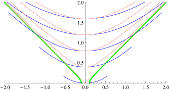
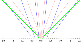
Figure 2: The top figure shows slices of constant FRW time, $\tau$ (red, light) and slices of constant geodesic time $t$ (blue, dark) in the vicinity of a bubble wall (green, thick) with initial size $r_{0}=0.1\,H_{\rm out}^{-1}$. Note that the constant $t$ slices are not defined for geodesics passing through the nucleation region of the bubble. The lower figure shows that geodesics of the congruence (blue, dark) eventually asymptote to comoving FRW worldlines (red, light).

Consider a region of the universe at late times, occupied by a “host” de Sitter vacuum with cosmological constant $3H_{\rm out}^{2}$. Let us suppose that $H_{\rm out}$ is very large, but far enough below the Planck scale to lend validity to our semiclassical treatment. Moreover, we suppose that a bubble of our own vacuum can form by a Coleman-DeLuccia (CDL) tunneling process inside the host vacuum.

Let us suppose, moreover, that the host vacuum has existed for many Hubble times $H_{\rm out}^{-1}$. Then, on the scale about to be occupied by a newly formed bubble, the geodesics emanating from the initial surface $\Sigma_{0}$ can be treated as comoving in the flat de Sitter metric

$$ds^{2}=-dt^{2}+H_{\rm out}^{-2}e^{2H_{\rm out}t}d{\mathbf{x}}^{2}$$ (4)

This follows, in a sense, from the de Sitter no-hair theorem; we will also find that it is consistent with our careful analysis in Sec. III.3.

Now suppose that a bubble of our vacuum forms at the time $t_{\rm nuc}$. It will appear at rest, with a proper radius $r_{0}\ll H_{\rm out}^{-1}$ determined by the CDL instanton. Then it will expand at constant acceleration $r_{0}^{-1}$, its world-volume asymptoting to a light-cone. Some of the above geodesics will eventually run into the bubble wall and enter our universe. Their behavior will determine the weight of any observations carried out inside the bubble, in the proper time measure.

We will not consider the small subset of geodesics that go through the nucleation region, $r\lesssim r_{0}$, where the classical geometry is not clearly defined. It is unclear how to treat these geodesics. This constitutes a challenge for the sharp formulation of congruence-based measures. The best we can say is that our results show that values of $r\sim O(r_{0})$ contribute negligibly to the measure as they are approached from above in a controlled regime. This could be viewed as evidence that the contribution of the uncontrolled regime can also be neglected.

The metric inside the bubble is given by an open FRW geometry; ignoring fluctuations, the metric is

$$ds^{2}=-d\tau^{2}+a(\tau)^{2}(d\xi^{2}+\sinh^{2}\xi\,d\Omega_{2}^{2})~{}.$$ (5)

where the scale factor $a(\tau)$ comprises, for anthropically relevant bubbles, a period of inflation followed by radiation, matter, and vacuum domination with very small cosmological constant. Note that $a(\tau)\approx\tau$ for sufficiently small $\tau$.

The maximally symmetric and negatively curved spatial slices defined by $\tau=const$ are physically preferred inside the bubble, since they correspond to hypersurfaces of (approximately) constant density. Only at very late times, well into the vacuum-dominated era, do we lose this preferred slicing, as the universe again becomes locally empty de Sitter.

The key point is that the preferred surfaces of constant FRW time $\tau$ are not the surfaces $\Sigma_{t}$ of constant geodesic time $t$. This is a complication, since $\tau$ is what we usually call the age of the universe, the time since the big bang—really, the metric distance from the bubble nucleation event. To the extent that any time variable is directly correlated with the outcome of an observation (such as CMB temperature or the amount of clustering), that variable will be the FRW time $\tau$, and not the global time $t$.

III.2 Square bubble approximation

The square bubble approximation, which is implicit in Ref. Lin06 , aims to circumvent this complication. It amounts to a deformation of the metric that allows us to calculate as if constant $\tau$ slices, inside the bubble, coincide with constant $t$ slices. For this we must arrange that the FRW time $\tau$ and the geodesic time $t$ differ only through a constant shift,

$$\tau=t-t_{\rm nuc}~{}.$$ (6)

This is possible only if the movement of the bubble wall is neglected.

Given this ad-hoc modification, the continuation of the geodesic congruence into the bubble cannot be directly computed. We will simply assume that the internal geometry of the new vacuum is a spatially finite piece of a flat FRW universe

$$ds^{2}=-d\tau^{2}+\tilde{a}(\tau)^{2}d{\mathbf{y}}^{2}~{}.$$ (7)

To match at $t=t_{\rm nuc}$ ($\tau=0$), we let ${\mathbf{y}}$ range over a finite physical volume $\tilde{a}(0)^{3}V_{y}$. We take the comoving volume to be independent of $\tau$, as if the bubble wall remained at fixed ${\mathbf{y}}$.

Note that both the scale factor and the initial size of the bubble initially differ significantly from their true values, and the matching to the outside fails at late times. However, in inflating vacua the exponential internal growth is more important than the expansion of the bubble forming their boundary. Moreover, inflation locally washes out the difference between a flat and an open universe. After a short time (say, a few e-foldings of inflation) we can take $\tilde{a}(\tau)\propto a(\tau)$.

Nevertheless, the square bubble approximation blatantly contradicts important known features, such as the fact that the constant-density slices inside are actually open and infinite. Indeed it is not even consistent geometrically, making it impossible to match the inside of the bubble to the outside. But one may hope that it gives a reasonable approximation for the purpose of computing probabilities. This will be the case if the approximation does not change the true count of observations of various types. We will find that the square bubble approximation is a good one for many questions.

III.3 Exact relation

The actual relation between the FRW coordinates $(\tau,\xi)$ and the geodesic proper time $t$ is more complicated. We set

$$H_{\rm out}=1\ \ {\rm in\ this\ subsection,}$$ (8)

so that the equations are not quite so ugly. In the outside flat deSitter slicing,

$$ds^{2}=-dt^{2}+e^{2t}\left(dr^{2}+r^{2}d\Omega_{2}^{2}\right)~{},$$ (9)

the domain wall follows the trajectory

$$r_{w}\exp(t_{w}-t_{\rm nuc}) = r_{0}\cosh\eta~{},$$ (10)

$$\exp(t_{w}-t_{\rm nuc}) = r_{0}\sinh\eta+\sqrt{1-r_{0}^{2}}~{}.$$ (11)

Here $r_{0}$ is the size of the bubble at nucleation; it is also the radius of curvature and the inverse proper acceleration of the domain wall. $r_{0}\eta$ is the proper time along the domain wall.

We need to compute the motion of geodesics as they cross the domain wall and live happily ever after in the interior. The natural coordinates inside the bubble are the open FRW coordinates $(\tau,\xi)$ of Eq. (5) because they respect the symmetry of the bubble nucleation. However, these coordinates do not cover the region containing the domain wall, so it is convenient to use a different coordinate system near the domain wall. Assuming that the Hubble constant in the interior of the bubble is much smaller than the Hubble constant in the exterior, we can find a scale $\tau^{*}$ such that $H_{\rm in}^{-1}\gg\tau^{*}\gg H_{\rm out}^{-1}$. The region from the domain wall to the $\tau^{*}$ surface is much smaller than the characteristic scales of the geometry inside the bubble. As a result, we can approximate it as a piece of Minkowski space. We will use coordinates in which the metric is

$$ds^{2}=-dT^{2}+dR^{2}+R^{2}d\Omega_{2}^{2}~{}.$$ (12)

Because the domain wall is a constant curvature surface with curvature radius $r_{0}$, its trajectory in the Minkowski coordinates is

$$R_{w} = r_{0}\cosh\eta~{},$$ (13)

$$T_{w} = r_{0}\sinh\eta~{},$$ (14)

where again $r_{0}\eta$ is the proper time along the domain wall. Computing the 4-velocity, we find that $\eta$ is the rapidity of the domain wall.

The trajectory of the geodesic after crossing the domain wall is

$$T = r_{0}\sinh\eta+(t-t_{w})\cosh\alpha~{},$$ (15)

$$R = r_{0}\cosh\eta+(t-t_{w})\sinh\alpha~{},$$ (16)

where $\alpha$ is the rapidity of the geodesic. We will determine $\alpha$ by demanding that the angle between the domain wall and the geodesic is continuous across the domain wall. If $u$ and $v$ are the 4-velocities of the geodesic and the domain wall, we demand

$$u\cdot v|_{\rm out}=u\cdot v|_{\rm in}~{}.$$ (17)

Since $\alpha$ is the rapidity of the geodesic and $\eta$ is the rapidity of the domain wall,

$$u\cdot v|_{\rm in}=\cosh(\eta-\alpha)~{}.$$ (18)

Geodesics outside the domain wall have a simple 4-velocity $u_{\rm out}=(1,0,0,0)$, and since we have identified $r_{0}\eta$ as the proper time along the domain wall, the 4-velocity of the domain wall is $v=({1\over r_{0}}~{}dt_{w}/d\eta,...)$. Using the equation (11) for the trajectory of the domain wall,

$$u\cdot v|_{\rm out}={1\over r_{0}}\frac{dt_{w}}{d\eta}=\frac{\cosh\eta}{r_{0}\sinh\eta+\sqrt{1-r_{0}^{2}}}~{}.$$ (19)

Thus the equation determining $\alpha$ is

$$\frac{\cosh\eta}{r_{0}\sinh\eta+\sqrt{1-r_{0}^{2}}}=\cosh(\eta-\alpha)~{}.$$ (20)

It is convenient to combine Eq. (20) and (11) to get

$$\cosh\eta\exp\left[-(t_{w}-t_{\rm nuc})\right]=\cosh(\eta-\alpha)~{}.$$ (21)

Simplifying we find

$$(t_{w}-t_{\rm nuc})=\alpha-\ln(1+\varepsilon)~{},$$ (22)

where

$$\varepsilon=\frac{e^{2\alpha}-1}{e^{2\eta}+1}~{}.$$ (23)

This is a convenient rewriting because one can show that $\varepsilon\ll 1$ for all geodesics as long as the critical bubble size is small in Hubble units, $r_{0}\ll 1$.

We want to rewrite the geodesics in terms of the open FRW coordinates which will be adapted to the cosmological evolution inside the bubble. For $\tau\ll H_{\rm in}^{-1}$, where the geometry is approximately Minkowski space, the relationship is

$$\tau = \sqrt{T^{2}-R^{2}}$$ (24)

$$\xi = \tanh^{-1}\frac{R}{T}~{}.$$ (25)

Using the trajectory in $(R,T)$ given by Eq. (15), (16), we find the trajectory in FRW coordinates

$$\xi = \alpha+{O}(\frac{1}{\tau})~{},$$ (26)

$$\tau = \sqrt{(t-t_{w})^{2}+2r_{0}(t-t_{w})\sinh(\eta-\xi)-r_{0}^{2}}~{}.$$ (27)

Our goal is to manipulate all of the above equations in order to find a single equation for the geodesic time since nucleation, $t-t_{\rm nuc}$, as a function of the natural coordinates $\tau,\xi$ inside the bubble.

We will be interested in events which occur a reasonable distance away from the domain wall, so that $\tau,t-t_{\rm nuc},t-t_{w}\gg 1$. So we can drop the subleading terms in (26) and just set the rapidity of the geodesic equal to the comoving coordinate, $\alpha=\xi$. Physically, the point is that the final comoving position of the geodesic is determined only by its velocity and not by its initial location. The nontrivial statement in (26) is that the geodesics become comoving in a time set by the Hubble scale outside the bubble, $H_{\rm out}^{-1}$.

In Eq. (27) we can now set $\alpha=\xi$ and expand for large $t-t_{w}$ to get

$$\tau=t-t_{w}+r_{0}\sinh(\eta-\xi)~{}.$$ (28)

Going back to (20) and solving for $\sinh(\eta-\xi)$ we find

$$\sinh(\eta-\xi)=\frac{\sqrt{1-r_{0}^{2}}\sinh\eta-r_{0}}{r_{0}\sinh\eta+\sqrt{1-r_{0}^{2}}}~{}.$$ (29)

Using the relation (11) between $\eta$ and $t_{w}$ this can be rewritten as

$$\sinh(\eta-\xi)={1\over r_{0}}\left[\sqrt{1-r_{0}^{2}}-\exp\left[-(t_{w}-t_{\rm nuc})\right]\right]~{}.$$ (30)

So we have an equation relating the geodesic time since nucleation to the FRW time $\tau$ and the time $t_{w}$ the geodesic crosses the domain wall:

$$\tau=t-t_{w}+\left[\sqrt{1-r_{0}^{2}}-\exp[-(t_{w}-t_{\rm nuc})]\right]~{}.$$ (31)

Now we can use the relation (22) between the rapidity $\alpha$ and $t_{w}$, together with $\alpha=\xi$, to get

$$\tau=t-t_{\rm nuc}-\bigg{[}\xi+e^{-\xi}-\sqrt{1-r_{0}^{2}}+\varepsilon e^{-\xi}-\ln(1+\varepsilon)\bigg{]}~{},$$ (32)

where $\varepsilon$ is given by (23). Expanding in $\varepsilon$ and restoring the factors of $H_{\rm out}$, we get the final formula relating the geodesic time to the natural coordinates inside the bubble:

$$t-t_{\rm nuc}=\tau+H_{\rm out}^{-1}\left[\xi+e^{-\xi}-1+...\right]~{}.$$ (33)

As expected, the difference between the geodesic proper time and the open FRW time depends non-trivially on the radial FRW coordinate $\xi$.

IV The spacetime location of a typical observer

The proper time measure makes nontrivial and interesting predictions for vacuum selection, which do not appear to contradict anything we know CliShe07 . However, as soon as we ask about the probabilities of different observations in the same vacuum, the measure wildly conflicts with observation. It has two properties that result in a squeeze. On the one hand, for an observation to be counted, it must occur before the cutoff $t$. On the other hand, the multiverse as a whole is expanding exponentially on a microscopic characteristic time scale. This makes it favorable to wait as long as possible until creating a low-energy, slowly expanding region like the one in which we are making our observations, and it strongly favors observations that happen soon after the fastest expanding vacuum has decayed. This is the general idea of the youngness paradox  LinLin96 ; Gut00a ; Gut00b ; Gut04 ; Teg05 ; Lin07 ; Gut07 .

We will present one explicit calculation to show the fact that, within bubbles identical to ours, the probability to live at $13.7$ Gyr is vanishingly small compared to the probability to live at $13$ Gyr. There is nothing new in this calculation, but it will be easier to see how the exact geometry we found goes into the paradox in Sec. IV.3, and how to analyze possible modifications in Sec. V.

Another manifestation of the youngness paradox is that if a number of tunneling events are necessary to get from the fastest inflating vacuum to our host vacuum, these successive tunneling events will tend to be separated by only the Planckian time interval $H_{\rm big}^{-1}$. Since the tunneling events are not well-separated, this renders it difficult to compute semiclassically. However, since such a quick succession of tunneling events does not obviously contradict observation, we sidestep this difficulty here by assuming that our vacuum is produced directly from the fastest inflating vacuum. Hence we set

$$H_{\rm out}=H_{\rm big}~{}.$$ (34)

This simplification makes the problem more well-defined; however, every indication is that the characteristic time scale appearing in the youngness paradox is $H_{\rm big}^{-1}$, regardless of this simplification.

IV.1 The youngness paradox in the square bubble approximation

We begin with an analysis in the square bubble approximation defined in Sec. III.2. By assumption, each bubble appears as a flat patch of the same physical size. Hence, the comoving volume $V_{x}$ taken up by a bubble in the outside metric goes like $\exp(-3H_{\rm big}t_{\rm nuc})$. Note, however, that we have rescaled the Euclidean spatial coordinates inside the bubble, $d{\mathbf{y}}=\exp(H_{\rm big}t_{\rm nuc})d{\mathbf{x}}$, so as to make the metric in each bubble explicitly the same (not just equivalent by diffeomorphism). In the sequel, “comoving volume” will usually refer to the inside metric and will accordingly be denoted $V_{y}$. It will be the same for each bubble, and so will drop out of probabilities.

Let $n(t)$ be the total number of bubbles of our type produced prior to the time $t$. This grows exponentially with time:

$$n(t)=C\exp(3H_{\rm big}t)~{}.$$ (35)

Here $C$ is a fixed constant, which depends on the size of $\Sigma_{0}$, the initial state, and the rate at which our vacuum is produced (directly or indirectly) by the fastest inflating vacuum. This constant will drop out in all ratios.

The nucleation of a bubble like ours will be followed by the formation of observers. Let $dN^{(1)}$ be the number of observations of some type, in a single bubble of our type, in a comoving volume of size $dV_{y}$ during the proper time interval $(\tau,\tau+d\tau)$ after the formation of the bubble. By the homogeneity of the FRW universe, $dN^{(1)}$ will depend only on the FRW time, $\tau$, so we can write

$$dN^{(1)}=f(\tau)\,d\tau\,dV_{y}~{}.$$ (36)

The function $f(\tau)$ can be thought of as an observer density.

As long as these observations involve looking out into the sky, they will usually be different at different times $\tau$. For simplicity, we begin by treating $\tau$ itself as an “observable”, and computing the probability density

$$\frac{dp}{d\tau}\propto\lim_{t\to\infty}\frac{dN}{d\tau}(t)~{}.$$ (37)

This is the probability for an observer to find themselves living a time $\tau$ after the big bang of their bubble.

Both the observer distribution, $f(\tau)$, and the volume per bubble, $V_{y}$, are the same for all bubbles of our type, by the above assumptions. Therefore, the total number of $\tau$-observations made by the time $t$ depends on $t$ only through the total number of bubbles $n(t-\tau)$ produced prior to the time $t-\tau$:

$$\frac{dN}{d\tau}(t) = n(t-\tau)\frac{dN^{(1)}}{d\tau}(\tau)=f(\tau)\,V_{y}\,n(t-\tau)$$ (38)

$$= f(\tau)\,V_{y}\,\exp\left[3H_{\rm big}(t-\tau)\right]~{}.$$

Since the $t$ dependence of the answer is just an overall normalization, it drops out of the probability distribution and we get the simple answer

$$\frac{dp}{d\tau}\propto f(\tau)\exp(-3H_{\rm big}\tau)~{}.$$ (39)

In our universe, it is reasonable to assume that $f(\tau)$ has a broad (at least Gyr-scale) peak at some $\tau_{\rm peak}\sim O(10$ Gyr$)$, since at early times, there was no structure, and at late times, there will be no free energy. In any case, there will be no features in $f(\tau)$ that can possibly compete with the exponential factor in Eq. (39), which suppresses the probability of late-time observations at a characteristic rate set by the microphysical scale $H_{\rm big}$.

For example, with Planckian $H_{\rm big}\sim O(1)$, there are at any time $t$

$$\frac{f(13\,{\rm Gyr})}{f(13.7\,{\rm Gyr})}\exp(10^{60})\approx\exp(10^{60})$$ (40)

observers who live 13 Gyr after their local big bang, for every observer like us. Thus, the probability of seeing a 13.7 Gyr old universe with a 2.7 K background temperature is vanishingly small compared to the observation of a warmer CMB and a somewhat younger universe.

This obviously contradicts experiment. Note that the probability for what we do see is so small that our observations so far are, by any standards applied in science, perfectly sufficient to rule out the theory—or in this case, the measure.

IV.2 Explicit conflict with observation

A possible objection to the above analysis is the fact that $\tau$, the time since the big bang in our bubble, is not a physical observable. Therefore, following Tegmark Teg05 , let us verify explicitly that the youngness paradox manifests itself in the probability distribution for physical observables.

Some observational consequences of the youngness pressure in this measure were described more than ten years ago by Linde, Linde, and Mezhlumian LinLin96 . There, the authors note that the proper time measure predicts that we are living at the center of an underdense region they refer to as an “infloid”. The effect they discuss arises because regions which spend less time in slow roll inflation (hence regions which reheat sooner and therefore are underdense) are rewarded. We focus here on a different effect which is more clearly in conflict with observation: the fact that typical observers see a different temperature than we do.

The probability distribution for the temperature is

$${dp\over dT}=\int d\tau{dp\over d\tau}g(T|\tau)~{},$$ (41)

where $g(T|\tau)$ is the probability distribution for temperatures at a fixed FRW time. For temperatures not too far from the average value,

$$g(T|\tau)\propto{1\over T_{\rm av}(\tau)}\exp\left[-10^{10}\left({T-T_{\rm av}(\tau)\over T_{\rm av}(\tau)}\right)^{2}\right]~{},$$ (42)

where $T_{\rm av}(\tau)$ is the average temperature at time $\tau$, and the factor of $10^{10}$ arises due to the magnitude of the density perturbations. The probability distribution becomes

$${dp\over dT}\propto\int d\tau{f(\tau)\over T_{\rm av}(\tau)}\exp\left[-3H_{\rm big}\tau-10^{10}\left({T-T_{\rm av}(\tau)\over T_{\rm av}(\tau)}\right)^{2}\right]~{}.$$ (43)

For the moment, let us ignore observations occurring before 10 Gyr, because for early enough times these formulas will break down. For the times under consideration, the average temperature satisfies

$${T_{\rm av}(\tau_{1})\over T_{\rm av}(\tau_{2})}=\left({\tau_{2}\over\tau_{1}}\right)^{2/3}~{}.$$ (44)

The probability distribution for temperature becomes

$${dp\over dT}\propto\int_{10~{}{\rm Gyr}}d\tau\,\tau^{2/3}f(\tau)\exp\left[-3H_{\rm big}\tau-10^{10}\left(\left(T\over 3.3K\right)\left(\tau\over 10~{}{\rm Gyr}\right)^{2/3}-1\right)^{2}\right]~{}.$$ (45)

The dominant factor in the integrand is $\exp(-3H_{\rm big}\tau)$, since this factor varies over the microphysical time scale $H_{\rm big}$, while the other factors vary on much larger time scales. Thus the integral is dominated by the lower limit. So the probability distribution for the temperature, once fluctuations are taken into account, is just equal to the distribution at the early time cutoff. Dropping a $T$-independent normalization factor, we find

$${dp\over dT}\propto g(T|\tau=10~{}{\rm Gyr})\propto\exp\left[-10^{10}\left({T-3.3K\over 3.3K}\right)^{2}\right]~{}.$$ (46)

It is easy to see that this prediction is ruled out at great confidence by our observation that $T=2.7$ K. The conflict only becomes worse as the early time cutoff is reduced.

IV.3 Exact treatment of the bubble geometry

In this subsection, we will improve on the above analysis by taking into account the actual dynamics and shape of bubble walls. Our treatment will clarify the extent to which the square-bubble approximation is justified, and confirm that the youngness paradox arises in the proper-time measure.

Inside a single bubble, as before we define a function $f(\tau)$ giving the number of observations per unit comoving volume per proper time,

$$dN^{(1)}=f(\tau)\,d\tau\,dV_{c}=f(\tau)\,4\pi\sinh^{2}\xi~{}d\xi\,d\tau~{}.$$ (47)

To get the total number of observations, $dN$, at given $(\tau,\xi)$, we must sum over all bubbles. We can organize this sum in terms of the time $t_{\rm nuc}<t$ when each bubble was nucleated. Note that given the coordinates $(\tau,\xi)$ inside the bubble, there is an upper limit $t_{\rm nuc}^{\rm max}(\tau,\xi)$ on the nucleation time so that the region of interest can be produced before the time $t$. This relationship was derived in Sec. (III.3). The sum becomes

$${dN\over d\tau d\xi}=\int_{0}^{t_{\rm nuc}^{\rm max}}dt_{\rm nuc}\left.\frac{dn}{dt}\right|_{t_{\rm nuc}}{dN^{(1)}\over d\tau d\xi}~{},$$ (48)

where the bubble production rate $dn/dt$ is still given by Eq. (35). Plugging in, we get

$${dN\over d\tau d\xi}=\int_{0}^{t_{\rm nuc}^{\rm max}}dt_{\rm nuc}\,C\exp\left(3H_{\rm big}t_{\rm nuc}\right)f(\tau)\,4\pi\sinh^{2}\xi$$ (49)

where, as derived in (33),

$$t_{\rm nuc}^{\rm max}=t-\tau-H_{\rm big}^{-1}\left(\xi+e^{-\xi}-1+...\right)~{}.$$ (50)

Performing the integral and dropping constant factors, we get

$${dN\over d\tau d\xi}=\left[e^{3H_{\rm big}t^{\rm max}_{\rm nuc}}-1\right]~{}f(\tau)\sinh^{2}\xi$$

$$= \left[e^{3H_{\rm big}\left[t-\tau-H_{\rm big}^{-1}(\xi+e^{-\xi}-1+...)\right]}-1\right]f(\tau)\,\sinh^{2}\xi$$

Taking the limit $t\to\infty$, we can ignore the “$-1$” coming from the lower limit of integration; in this limit the $t$ dependence is only an overall multiplicative factor which vanishes upon normalization. Thus we obtain a simple formula for the probability distribution

$${dN\over d\xi d\tau}=f(\tau)e^{-3H_{\rm big}\tau}~{}\sinh^{2}\xi e^{-3(\xi+e^{-\xi}-1+...)}$$ (52)

The striking feature of this probability distribution is that it factorizes into a function of the spatial coordinate $\xi$ times a function of the FRW time $\tau$. This is exactly true, because the “$\ldots$” appearing in the formula is a function of $\xi$ only.

The distribution as a function of $\tau$ is given by

$$\frac{dp}{d\tau}\propto f(\tau)e^{-3H_{\rm big}\tau}~{}.$$ (53)

This distribution is exactly the same as Eq. (39), which was derived in the square bubble approximation. So the youngness paradox appears in exactly the same way in the true geometry.

The spatial distribution of observers at a fixed FRW time $\tau$ is

$$\frac{dp}{d\xi}\propto\sinh^{2}\xi\exp\left[-3(\xi+e^{-\xi}-1+...)\right]$$ (54)

This distribution peaks at $\xi$ of order one, and falls exponentially for large $\xi$. So most observers live within a few curvature radii of the “center of the universe.” The center is defined by the geodesic piercing the bubble nucleation point.

IV.4 Why did the square bubble approximation work?

The main effect of the correctly computed probability distribution over $\xi$ is to allow only an effective comoving volume

$$V_{\xi,{\rm eff}}=4\pi\int_{0}^{\infty}d\xi\sinh^{2}\xi\exp\left[-3(\xi-1+e^{-\xi})\right]\approx 15.75$$ (55)

to contribute for every bubble.

The above result could not have been computed in the square bubble approximation, but it explains why that approximation worked for computing the temporal distribution of observers. The point is that in a large regime, it is possible to identify the finite spatial region containing typical observers with the finite flat patch of “new vacuum” inserted by hand in the square bubble approximation.

This identification is not a true match, because of the different spatial curvature. But during and after inflation, there is a long period where curvature is negligible and the scale factor would be the same function of time in a flat FRW universe. If the observations contributing to the measure occur in this regime, then the use of spatially flat time-slices in the square-bubble approximation will be legitimate.

The effective physical volume at large FRW time $\tau$ is $15.75\,a^{3}(\tau)$. During inflation, $a(\tau)=H_{\rm inf}^{-1}\sinh H_{\rm inf}\tau$. To match this to the square bubble physical volume, $V_{y}H_{\rm inf}^{-3}\exp\left(3H_{\rm inf}\tau\right)$, at $\tau\gg H_{\rm inf}^{-1}$, requires the choice

$$V_{y}=V_{\xi,{\rm eff}}/8\approx 2~{}.$$ (56)

Note that in a problem involving different types of bubbles, the physical volume of a new bubble will be of order $H_{\rm inf}^{-3}$. Generically $H_{\rm inf}$ will be smaller than the outside Hubble constant. If we took Eq. (56) literally, the square bubble approximation would involve replacing a large number of outside Hubble volumes with the new vacuum. This contradicts the geometric fact that asymptotically, the new bubble takes up the comoving volume occupied by only one outside Hubble volume at the time of nucleation. Of course, the choice of $V_{y}$ dropped out of ratios, so it could be reduced without affecting relative probabilities.

In any case, while the square bubble approximation turned out to be a useful shortcut under the above assumptions, it is just as simple, and much more reliable, to use the exact geometry, as encoded in Eq. (32), to compute probabilities.

V Modifications of the proper time measure

Obviously, the result that practically all observers live at a much earlier time, and see a very different universe, than we do, is fatal for the proper time measure. Perhaps the measure can be modified in some way, so as to avoid this problem?

V.1 Don’t ask, don’t tell

Linde advocates a simple resolution to the youngness paradox in Ref. Lin06 (see also references therein). One should simply not ask how long after reheating the typical observers form, but merely compute the rate at which reheating hypersurfaces of different inflating vacua are produced. This restriction has a number of problems. If we cannot ask about the temperature measured by a typical observer, the measure is not complete. Moreover, if we cannot ask about observers, then we cannot count them, and so we cannot condition on their number. This would eliminate the anthropic solution to the cosmological constant problem. And finally, as noted in Ref. Lin07 , this restriction does not fully solve the youngness problem in any case. It merely confines the problem to effects before reheating. In particular, it gives overwhelming weight to vacua with a shorter period of inflation, and thus predicts a wide open universe. Thus, a different modification is needed.

A general idea for such a fix was outlined in Ref. Lin07 : “One should compare apples to apples, instead of comparing apples to the trunks of the trees.” In other words, we should assign a correction factor $e^{3H_{\rm big}\Delta t_{i}}$ to the probability $p_{i}$ for the observation $O_{i}$, where $\Delta t_{i}$ is the amount of time it takes to produce such an observation, in some relative sense to be defined below. The corrected relative probabilities are thus:

$$\frac{P(O_{1})}{P(O_{2})} = \frac{p(O_{1})}{p(O_{2})}\exp[3H_{\rm big}(\Delta t_{1}-\Delta t_{2})]$$

$$= \lim_{t\to\infty}\frac{N_{1}(t)}{N_{2}(t)}\exp[3H_{\rm big}(\Delta t_{1}-\Delta t_{2})]~{}.$$

Compared to Eq. (1), this bolsters mature folk like ourselves, by compensating for the enormous volume growth that Boltzmann babies can take advantage of.

No general, sharp definition of $\Delta t_{i}$ was attempted in Ref. Lin07 , where explicit calculations were carried out only for a model containing two vacua with different lengths of inflation; $\Delta t_{i}$ was defined to be the duration of inflation in each vacuum. While Ref. Lin07 claimed that the procedure also resolves other aspects of the youngness paradox, such as the overwhelming probability for a hotter universe, it offered no definition of $\Delta t$ in that context, nor did it display an explicit computation of the corrected probability.

In fact, we have been unable to come up with a general definition of $\Delta t$ that succeeds in fixing the youngness problem. This does not mean that it cannot be done. But perhaps it will help sharpen the challenge if we discuss a few proposals that may come to mind.

V.2 Spatial averaging

The prediction that we should observe a warmer CMB temperature arose from the fact that it takes longer to produce observers who see low CMB temperatures. To get a more reasonable probability distribution for the CMB temperature, we want to eliminate the enormous cost of waiting for the universe to cool off. It seems reasonable to assign $\Delta t(T)$ as the amount of FRW time until the average background temperature is $T$. Since we will only be comparing observations within the same bubble and after reheating, an additive constant in $\Delta t$ is unimportant and so we can start our clock at any time we like.

We explore this proposal mostly because it seems like the most straightforward and naive fix. In fact, it is unclear how the above definition would generalize to observables that can take on the same value at very different times. Even for the temperature, small perturbations render the relation between its average value and a particular time slice ambiguous at the $10^{-5}$ level—much too large to define $\Delta t$ with the required Planckian precision. We will disregard all these issues, since the modification fails even in the idealized special case we consider.

For temperatures and times close to those we observe, the average temperature on $\tau=$ const slices satisfies

$${T(\tau_{1})\over T(\tau_{2})}=\left({\tau_{2}\over\tau_{1}}\right)^{2/3}~{}.$$ (58)

Thus, $\Delta t(T)$ is given by

$$\Delta t(T)=(13.7~{}{\rm Gyr})\left(2.7~{}{\rm K}\over T\right)^{3/2}~{}.$$ (59)

The modification fails because it is comparatively easy to find deviations from the average temperature. To see this, let us begin by considering a further idealization: Let us exclude fluctuations of $T$. In other words, we will assume that the CMB temperature, at fixed $\tau$, is given everywhere precisely by the same value.

With this additional idealization, the modification actually works! There is now a one-to-one correspondence between $\tau$ and $T$, so we can use Eq. (39) to obtain the (unmodified) probability distribution for $T$:

$${dp\over dT}={dp\over d\tau}{d\tau\over dT}\propto f(\tau(T)){d\tau\over dT}\exp\left[-3H_{\rm big}\tau(T)\right]$$ (60)

where $f(\tau)$, as before, is the rate of observations per comoving volume per unit time per bubble. The quantity $f(\tau(T)){d\tau\over dT}$ is naturally identified as $f(T)$, the rate of observations per comoving volume per unit background temperature per bubble. Using the previous formula relating time to temperature, we find

$${dp\over dT}\propto f(T)\exp\left[-3H_{\rm big}\cdot(13.7~{}{\rm Gyr})\left(2.7~{}{\rm K}\over T\right)^{3/2}\right]~{}.$$ (61)

Still working in the idealization of exactly homogeneous background temperature, let us now compute the modified probability distribution for temperature. It is

$${dP\over dT}\propto f(T)\exp\left[-3H_{\rm big}(\tau(T)-\Delta t(T))\right]$$ (62)

We have defined $\Delta t$ so that the exponent is zero, so the modified probability distribution for temperature is simply proportional to the number of observations at each temperature,

$${dP\over dT}\propto f(T)~{}.$$ (63)

This answer seems intuitive and has no youngness problem. (See, however, the discussion at the end of Sec. V.5.)

Once we allow for fluctuations of the temperature, $\Delta t(T)$ can still be defined in terms of the average temperature. But our recipe for repairing the probabilities no longer works.

Now the starting point is the (unmodified) probability distribution obtained in Sec. IV.2, Eq. (46). After applying Eq. (V.1), with $\Delta t(T)$ given by Eq. (59), we obtain the modified distribution

$${dP\over dT}=\exp\left[3H_{\rm big}\Delta t(T)\right]g(T|\tau=10~{}{\rm Gyr})$$ (64)

Using

$$\Delta t(T)=(10~{}{\rm Gyr})\left(3.3K\over T\right)^{3/2}~{},$$ (65)

and assuming Planckian $H_{\rm big}$, we get

$${dP\over dT}=\exp\left[10^{61}\left(3.3K\over T\right)^{3/2}-10^{10}\left({T-3.3K\over 3.3K}\right)^{2}\right]$$ (66)

The temperature is now driven to the lowest possible value. It is still favorable to live early, and because of the primordial density fluctuations, it is not all that hard to find an anomalously cool region even at early times. Our modification factor rewards us for this as if we had honestly waited until the average temperature becomes so low. Thus, it overcompensates.

This new distribution is also ruled out, at enormous confidence level, by our observation of 2.7 K.

V.3 Waiting for the first time

Another possibility is to define $\Delta t_{i}$ for the observation of type $O_{i}$ as the time it takes the universe, starting from the beginning of time (the slice $\Sigma_{0}$), to produce the first such observation.

Thus defined, $\Delta t_{i}$—and hence, the corrected probabilities—will depend on the initial conditions on $\Sigma_{0}$. This dependence may be mild, and in any case we can see no reason why probabilities (at least for some observables) should not depend on the initial conditions of the universe. However, if we define $\Delta t_{i}$ as the time when $N_{i}$ jumps from 0 to 1, then it will also depend on accidents of the semiclassical evolution at early times, such as the time when a particular tunneling event happens to take place, and we would not be able to compute it directly from the theory.

This problem can be resolved by defining $\Delta t_{i}$ to be the time when the expectation value $\langle N_{i}(\Delta t)\rangle$ becomes 1. This still depends on initial conditions but can be computed from the theory in the semiclassical regime.

However, this definition conflicts with an important property of probabilities. Consider the special case that $O_{1}$ and $O_{2}$ are mutually exclusive outcomes of an experiment. For example, outcome $O_{1}$ ($O_{2}$) may be up (down) when the spin of a single electron is measured by a man in a penguin suit. In general there may be additional possible outcomes $O_{3},\ldots$, but in any case, it must be true that

$$p_{1}+p_{2}=p_{12}~{},$$ (67)

where $p_{12}$ is the probability for the outcome “1 or 2”. Indeed, this property will be satisfied by the original probabilities defined in Eq. (1).

However, $\Delta t_{12}<\Delta t_{i}$, $i=1,2$, because the expected time when “1 or 2” is first observed is simply the time when the experiment is first likely to be performed. This is sooner than the expected time when, say, 1 is first observed, since the very first experiment can only have one outcome. Therefore, the corrected probabilities do not add up correctly:

$$P_{1}+P_{2} = p_{1}e^{3H_{\rm big}\Delta t_{1}}+p_{2}e^{3H_{\rm big}\Delta t_{2}}$$

$$> (p_{1}+p_{2})e^{3H_{\rm big}\Delta t_{12}}=P_{12}~{},$$

Another way of saying this is that we can change the total probability for a set of alternative outcomes by whether we view the alternatives separately and add probabilities, or group the alternatives together and directly compute the probability for this compound outcome. This is clearly absurd.

A particularly simple and striking result obtains if we assume initial conditions that are already in the stationary regime. Then

$$\langle N_{i}(t)\rangle=Vp_{i}(e^{3H_{\rm big}t}-1)~{}.$$ (69)

The uncorrected probabilities $p_{i}$ are dynamically determined by the attractor behavior; the overall scaling $V$ depends on the volume of $\Sigma_{0}$. We find for the correction factor

$$e^{3H_{\rm big}\Delta t_{i}}=\frac{Vp_{i}+1}{Vp_{i}}~{},$$ (70)

and hence

$$\frac{P_{i}}{P_{j}}=\frac{Vp_{i}+1}{Vp_{j}+1}.$$ (71)

In the large volume limit, there is no correction and the youngness paradox persists. For finite $V$, the corrected probabilities do not obey $P_{1}+P_{2}=P_{12}$. In the limit $V\to 0$, all alternatives become equally likely, $P_{i}/P_{j}=1$, no matter how they were defined!

V.4 Growing together

A different definition for $\Delta t_{i}$ may be motivated by another quote from Ref. Lin07 : $\Delta t_{i}$ is “the time when the stationary regime becomes established” for the observation $O_{i}$. Mathematically, we may attempt to capture this idea as follows. At late times, we know that the number of observations of any type will grow as $e^{3H_{\rm big}t}$, so $\dot{N}_{i}/N_{i}\to 3H_{\rm big}$. At any finite time, there will be a small correction to this time dependence, so we may define $\delta t_{i}$ as the earliest time when

$$\left|1-\frac{\dot{N}_{i}(t_{i})}{3H_{\rm big}N_{i}(t_{i})}\right|\leq\epsilon~{}.$$ (72)

It would seem arbitrary to specify an particular small deviation $\epsilon$ beyond which we consider the stationary regime established. Therefore, let us take the limit $\epsilon\to 0$. In this limit each $\delta t_{i}$ contains the same additive divergence, $-\log\epsilon$, which we discard and define

$$\Delta t_{i}=\lim_{\epsilon\to 0}\delta t_{i}+\log\epsilon~{}.$$ (73)

To see that this measure does not work, let us focus again on the CMB temperature in our own vacuum. For the sake of argument, suppose that no observers exist prior to some cutoff FRW time, say, $\tau_{\rm min}=10$ Gyr. By the results of Sec. IV.2, for any finite geodesic time $t$, practically all observations of any value of $T$ are made within a time of order $H_{\rm big}^{-1}$ after $\tau_{\rm min}$. Therefore, to accuracy $H_{\rm big}^{-1}$, $|1-{\dot{N}_{T}}/(3H_{\rm big}N_{T})|$ will drop below $\epsilon$ at the same time $t$, for any temperature $T$. Hence, $\Delta t_{T}$ is independent of $T$ to this accuracy. Therefore, our “modification” does not in fact change relative probabilities at all.

To complete this argument, we should now take the cutoff FRW time, $\tau_{\rm min}$, earlier and earlier, until it is removed altogether. However, this introduces only information about early universe physics into our modification of the proper time measure. It cannot possibly restore a reasonable probability distribution for the CMB temperature measured by observers in the present era.

It is interesting that like “spatial averaging”, the present modification would have worked for (fictitious) observables that are in one-to-one correspondence with the FRW time. In this case, it would not have been true that at any time $\tau$, there is a nonzero amplitude for any temperature $T$. Instead,

$$N_{T_{1}}(t)=\frac{f(T_{1})}{f(T_{2})}N_{T_{2}}(t+\tau(T_{2})-\tau(T_{1}))~{},$$ (74)

and hence,

$$\frac{\dot{N}_{T_{1}}}{N_{T_{1}}}(t)=\frac{\dot{N}_{T_{2}}}{N_{T_{2}}}(t+\tau(T_{2})-\tau(T_{1}))~{}.$$ (75)

Then we would have found

$$\Delta t_{1}-\Delta t_{2}=\Delta t(T_{1})-\Delta t(T_{2})~{},$$ (76)

and we would have recovered the intuitive result of Eq. (63).

Apparently, the problem with both of these modifications is that the value of an observable does not give us enough information about the FRW time when the observation is made—but this is precisely the time we would like to use for $\Delta t$. This motivates our final attempt at modifying the proper time measure, in which $\Delta t$ is defined not as a function of observables, but directly as a function of the time when the observation is made, regardless of its outcome.

V.5 Anticipation

Instead of tying $\Delta t$ to a specific observable, we can go back and fix the time shift directly for the geodesics. Effectively, it is like “anticipating” all observations that will happen in a given bubble. More precisely, let us project every observation $$

- (1) J. B. Hartle and M. Srednicki: Are we typical?. Phys. Rev. D 75, 123523 (2007), arXiv:0704.2630 [hep-th].
- (2) D. N. Page: Typicality defended (2007), arXiv:0707.4169 [hep-th].
- (3) J. Garriga and A. Vilenkin: Prediction and explanation in the multiverse (2007), arXiv:0711.2559 [hep-th].
- (4) R. Bousso and J. Polchinski: Quantization of four-form fluxes and dynamical neutralization of the cosmological constant. JHEP 06, 006 (2000), hep-th/0004134.
- (5) J. Polchinski: The cosmological constant and the string landscape (2006), hep-th/0603249.
- (6) R. Bousso: TASI lectures on the cosmological constant (2007), arXiv:0708.4231 [hep-th].
- (7) S. Coleman and F. D. Luccia: Gravitational effects on and of vacuum decay. Phys. Rev. D 21, 3305 (1980).
- (8) A. H. Guth and E. J. Weinberg: Could the universe have recovered from a slow first-order phase transition?. Nucl. Phys. B212, 321 (1983).
- (9) R. Bousso: Holographic probabilities in eternal inflation. Phys. Rev. Lett. 97, 191302 (2006), hep-th/0605263.
- (10) J. Garriga, A. H. Guth and A. Vilenkin: Eternal inflation, bubble collisions, and the persistence of memory (2006), hep-th/0612242.
- (11) B. Freivogel and L. Susskind: A framework for the landscape (2004), hep-th/0408133.
- (12) B. Freivogel, Y. Sekino, L. Susskind and C.-P. Yeh: A holographic framework for eternal inflation. Phys. Rev. D 74, 086003 (2006), hep-th/0606204.
- (13) L. Susskind: The census taker’s hat (2007), arXiv:0710.1129 [hep-th].
- (14) A. Maloney, S. Shenker and L. Susskind: unpublished ().
- (15) A. Vilenkin: Probabilities in the landscape (2006), hep-th/0602264.
- (16) A. Linde: Sinks in the landscape, Boltzmann Brains, and the cosmological constant problem. JCAP 0701, 022 (2007), hep-th/0611043.
- (17) V. Vanchurin: Geodesic measures of the landscape. Phys. Rev. D 75, 023524 (2007), hep-th/0612215.
- (18) J. Garriga, D. Schwartz-Perlov, A. Vilenkin and S. Winitzki: Probabilities in the inflationary multiverse. JCAP 0601, 017 (2006), hep-th/0509184.
- (19) D. N. Page: Is our universe likely to decay within 20 billion years? (2006), hep-th/0610079.
- (20) R. Bousso and B. Freivogel: A paradox in the global description of the multiverse. JHEP 06, 018 (2007), hep-th/0610132.
- (21) A. Vilenkin: Freak observers and the measure of the multiverse. JHEP 01, 092 (2007), hep-th/0611271.
- (22) D. N. Page: Return of the Boltzmann brains (2006), hep-th/0611158.
- (23) D. Schwartz-Perlov and A. Vilenkin: Probabilities in the Bousso-Polchinski multiverse. JCAP 0606, 010 (2006), hep-th/0601162.
- (24) K. D. Olum and D. Schwartz-Perlov: Anthropic prediction in a large toy landscape (2007), arXiv:0705.2562 [hep-th].
- (25) R. Bousso and I.-S. Yang: Landscape predictions from cosmological vacuum selection. Phys. Rev. D 75, 123520 (2007), hep-th/0703206.
- (26) R. Bousso, R. Harnik, G. D. Kribs and G. Perez: Predicting the cosmological constant from the causal entropic principle. Phys. Rev. D 76, 043513 (2007), hep-th/0702115.
- (27) J. M. Cline, A. R. Frey and G. Holder: Predictions of the causal entropic principle for environmental conditions of the universe (2007), arXiv:0709.4443 [hep-th].
- (28) A. Linde: Eternally existing selfreproducing chaotic inflationary universe. Phys. Lett. B175, 395 (1986).
- (29) A. Linde, D. Linde and A. Mezhlumian: From the big bang theory to the theory of a stationary universe. Phys. Rev. D 49, 1783 (1994), gr-qc/9306035.
- (30) J. García-Bellido, A. Linde and D. Linde: Fluctuations of the gravitational constant in the inflationary Brans-Dicke cosmology. Phys. Rev. D 50, 730 (1994), astro-ph/9312039.
- (31) J. Garcia-Bellido and A. D. Linde: Stationarity of inflation and predictions of quantum cosmology. Phys. Rev. D51, 429 (1995), hep-th/9408023.
- (32) J. García-Bellido and A. Linde: Stationary solutions in Brans-Dicke stochastic inflationary cosmology. Phys. Rev. D 52, 6730 (1995), gr-qc/9504022.
- (33) A. Linde, D. Linde and A. Mezhlumian: Nonperturbative amplifications of inhomogeneities in a self-reproducing universe. Phys. Rev. D 54, 2504 (1996), gr-qc/9601005.
- (34) A. H. Guth: Inflation and eternal inflation. Phys. Rep. 333, 555 (1983), astro-ph/0002156.
- (35) A. H. Guth: Inflationary models and connections to particle physics (2000), astro-ph/0002188.
- (36) A. H. Guth: Inflation (2004), astro-ph/0404546.
- (37) M. Tegmark: What does inflation really predict?. JCAP 0504, 001 (2005), astro-ph/0410281.
- (38) A. Linde: Towards a gauge invariant volume-weighted probability measure for eternal inflation. JCAP 0706, 017 (2007), arXiv:0705.1160 [hep-th].
- (39) A. H. Guth: Eternal inflation and its implications. J. Phys. A40, 6811 (2007), hep-th/0702178.
- (40) R. M. Wald: General Relativity. The University of Chicago Press, Chicago (1984).
- (41) A. D. Linde: Particle physics and inflationary cosmology. Harwood, Chur, Switzerland (1990).
- (42) R. Bousso, B. Freivogel and I.-S. Yang: Eternal inflation: The inside story. Phys. Rev. D 74, 103516 (2006), hep-th/0606114.
- (43) T. Clifton, S. Shenker and N. Sivanandam: Volume weighted measures of eternal inflation in the Bousso-Polchinski landscape (2007), arXiv:0706.3201 [hep-th].
- (44) L. Dyson, M. Kleban and L. Susskind: Disturbing implications of a cosmological constant. JHEP 10, 011 (2002), hep-th/0208013.