Electronic properties of bilayer and multilayer graphene

Abstract

We study the effects of site dilution disorder on the electronic properties in graphene multilayers, in particular the bilayer and the infinite stack. The simplicity of the model allows for an easy implementation of the coherent potential approximation and some analytical results. Within the model we compute the self-energies, the density of states and the spectral functions. Moreover, we obtain the frequency and temperature dependence of the conductivity as well as the DC conductivity. The c-axis response is unconventional in the sense that impurities increase the response for low enough doping. We also study the problem of impurities in the biased graphene bilayer.

I Introduction

The isolation of single layer graphene by Novoselov et al. Novoselov et al. (2004) has generated enormous interest in the physics community. On the one hand, the electronic excitations of graphene can be described by the two-dimensional (2D) Dirac equation, creating connections with certain theories in particle physics.Castro Neto et al. (2006) Moreover, the “relativistic” nature of the quasiparticles, albeit with a speed of propagation, $v_{F}$, 300 times smaller than the speed of light, leads to unusual spectroscopic, transport, and thermodynamic properties that are at odds with the standard Landau-Fermi liquid theory of metals.Castro Neto et al. (2007) On the other hand, graphene opens the doors for an all-carbon based micro-electronics.Geim and Novoselov (2007)

Due to the strong nature of the $\sigma$ bonds in graphene, and strong mechanical stability of the graphene lattice, miniaturization can be obtained at sizes of order of a few nanometers, beyond what can obtained with the current silicon technology (the smallest size being of the order of the benzene molecule). Furthermore, the same stability allows for creation of entire devices (transistors, wires, and contacts) carved out of the same graphene sheet, reducing tremendously the energy loss, and hence heating, created by contacts between different materials.Berger et al. (2004) Early proposals for the control of the electronic properties in graphene, such as the opening of gaps, were based on controlling its geometry, either by reducing it to nanoribbons,Nakada et al. (1996) or producing graphene quantum dots.Silvestrov and Efetov (2007) Nevertheless, current lithographic techniques that can produce such nanostructures do not have enough accuracy to cut graphene to Ångstrom precision. As a result, graphene nanostructures unavoidably have rough edges which have strong effects in the transport properties of nanoribbons.Han et al. (2007) In addition, the small size of these structures can lead to strong enhancement of the Coulomb interaction between electrons which, allied to the disorder at the edge of the nanostructures, can lead to Coulomb blockade effects easily observable in transport and spectroscopy.Sols et al. (2007)

Hence, the control of electronic gaps by finite geometry is still very unreliable at this point in time and one should look for control in bulk systems which are insensitive to edge disorder. Fortunately, graphene is an extremely flexible material from the electronic point of view and electronic gaps can be controlled. This can be accomplished in a graphene bilayer with an electric field applied perpendicular to the plane. It was shown theoretically McCann and Fal’ko (2006); McCann (2006) and demonstrated experimentally Castro et al. (2007a); Oostinga et al. (2007) that a graphene bilayer is the only material with semiconducting properties that can be controlled by electric field effect. The size of the gap between conduction and valence bands is proportional to the voltage drop between the two graphene planes and can be as large as $0.1-0.3$ eV, allowing for novel terahertz devicesCastro et al. (2007a) and carbon-based quantum dotsJ. Milton Pereira et al. (2007) and transistors.Nilsson et al. (2007)

Nevertheless, just as single layer graphene,Peres et al. (2006) bilayer graphene is also sensitive to the unavoidable disorder generated by the environment of the SiO₂ substrate: adatoms, ionized impurities, etc. Disorder generates a scattering rate $\tau$ and hence a characteristic energy scale $\hbar/\tau$ which is the order of the Fermi energy $E_{F}=\hbar v_{F}k_{F}$ ($k_{F}\propto\sqrt{n}$ is the Fermi momentum and $n$ is the planar density of electrons) when the chemical potential is close to the Dirac point ($n\to 0$). Thus, one expects disorder to have a strong effect in the physical properties of graphene. Indeed, theoretical studies of the effect of disorder in unbiased Nilsson et al. (2006a) and biased Nilsson and Castro Neto (2007) graphene bilayer (and multilayer) show that disorder leads to strong modifications of its transport and spectroscopic properties. The understanding of the effects of disorder in this new class of materials is fundamental for any future technological applications. In this context it is worth to mention the transport theories based on the Boltzmann equation,Katsnelson (2007); Adam and Sarma a study of weak localization in bilayer graphene,Kechedzhi et al. (2007) and also corresponding further experimental characterization.Morozov et al. ; Gorbachev et al. (2007) DC transport in few-layer graphene systems have been studied in Ref. Nakamura and Hirasawa, , both without and in the presence of a magnetic field.

In this paper, we study the effects of site dilution (or unitary scattering) on the electronic properties of graphene multilayers within the well-known coherent potential approximation (CPA). While the CPA does not take into account electron localization,not ; Ziegler (2006) it does provide quantitative and qualitative information on the effect of disorder in the electronic excitations. Furthermore, this approximation allows for analytical results of electronic self-energies, allowing us to compute physical quantities such as spectral functions (measurable by angle resolved photoemission, ARPES Zhou et al. (2006a, b); Bostwick et al. (2007); Ohta et al. (2006); Zhou et al. (2007)) and density of states (measurable by scanning tunneling microscopy, STMStolyarova et al. (2007); Mallet et al. (2007); Li and Andrei (2007); Brar et al. (2007)), besides standard transport properties such as the DC and AC conductivities.Nilsson et al. (2006a) Furthermore, in the case of the semi-infinite stack of graphene planes we can compute the c-axis response of the system which is rather unusual since it increases with disorder at low electronic densities, in agreement with early transport measurements in graphite.Brandt et al. (1988)

The paper is organized as follows. In Sec. II we discuss the band model of the graphene bilayer within the tight-binding approximation. We also connect our notation with the one established for graphite, namely the Slonsczewki-Weiss-McClure (SWM) parameterization. In Sec. III we introduce several simplified band models and compare the electronic bands in different approximations. The Green’s functions that we use later on in the paper are given in Sec. IV.

We employ a simplified model for the disordered graphene bilayer in Sec. V and work out the consequences on the single particle properties encoded in the self-energies, the density of states (DOS) and the spectral function. Sec. VI contains results for the graphene multilayer. In Sec. VII we introduce the linear response formulas that we use to calculate the electronic and optical response. The results for the conductivities in the bilayer are presented in Sec. VIII, while those for the multilayer can be found in Sec. IX.

The rest of the paper concerns the problem of impurities in the biased graphene bilayer. The model of the system and some of its basic properties are discussed in Sec. X. In Sec. XI we solve the problem of a Dirac delta impurity exactly within the effective mass approximation. A simple estimate of when the interactions among impurities becomes important is presented in Sec. XII. We treat more general impurity potentials with variational methods in Sec. XIII, and the special case of a potential well with finite range is studied in Sec. XIV. In Sec. XV we study the problem of a finite density of impurities in the coherent potential approximation (CPA). The effects of trigonal distortions on our results for the biased graphene bilayer are discussed briefly in Sec. XVI. Finally, the conclusions of the paper are to be found in Sec. XVII. We have also included four appendices with technical details of the calculations of the minimal conductivity in bilayer graphene (App. A), the DOS in multilayer graphene (App. B), the conductivity kernels (App. C), and the Green’s function in the biased graphene bilayer (App. D).

II Electronic bands of the graphene bilayer

Many of the special properties of the graphene bilayer have their origin in its lattice structure that leads to the peculiar band structure that we discuss in detail in this section. A simple way of arriving at the band structure of the graphene bilayer is to use a tight-binding approximation. The positions of the different atoms in the graphene bilayer are shown in Fig. 1 together with our labeling convention.

The advantage of this notation is that one can discuss collectively about the A (B) atoms that are equivalent in their physical properties such as the weight of the wave functions and the distribution of the density of states etc. This notation was used in early work on graphite.McClure (1957); Slonczewski and Weiss (1958) Many authors use instead a notation similar to $\text{A}1\rightarrow\text{A}$, $\text{B}1\rightarrow\text{B}$, $\text{A}2\rightarrow\widetilde{\text{B}}$, and $\text{B}2\rightarrow\widetilde{\text{A}}$. In this notation the relative orientation within the planes of the A ($\widetilde{\text{A}}$) and B ($\widetilde{\text{B}}$) atoms are the same; but for the other physical properties the equivalent atoms are instead A (B) and $\widetilde{\text{B}}$ ($\widetilde{\text{A}}$). Because the other physical properties are often more relevant for the physics than the relative orientation of the atoms within the planes we choose to use the, in our view, most “natural” labeling convention.

II.1 Monolayer graphene

Let us briefly review the tight-binding model of monolayer graphene.Wallace (1947) The band structure can be described in terms of a triangular lattice with two atoms per unit cell. The real-space lattice vectors can be taken to be ${\bf a}_{1}=\frac{a}{2}(3,\sqrt{3})$ and ${\bf a}_{2}=\frac{a}{2}(3,-\sqrt{3})$. Here $a$ ($\approx 1.4\,\text{\AA}$) denotes the nearest neighbor carbon distance. Three vectors that connect atoms that are nearest neighbors are ${\bm{\delta}}_{1}=\frac{a}{2}(1,\sqrt{3})$, ${\bm{\delta}}_{2}=\frac{a}{2}(1,-\sqrt{3})$, and ${\bm{\delta}}_{3}=a(-1,0)$; we take these to connect the $\text{A}1$ atoms to the $\text{B}1$ atoms. In terms of the operators that creates (annihilates) an electron on the lattice site at position ${\bf R}_{i}$ and lattice site $\alpha j$ [ $\alpha=(\text{A},\,\text{B})$ denotes the atom sublattice and $j$ ($j=1$) denotes the plane ]: $c_{\alpha j,{\bf R}_{i}}^{{\dagger}}$ ($c_{\alpha j,{\bf R}_{i}}^{\ }$), the tight-binding Hamiltonian reads:

$$H_{\text{t.b.}}=t\sum_{{\bf R}_{i}}\sum_{j=1,2,3}\bigl{(}c_{\text{A}1,{\bf R}_{i}}^{{\dagger}}c_{\text{B}1,{\bf R}_{i}+\bm{\delta}_{j}}^{\ }+\text{h.c.}\bigr{)}.$$ (1)

Here $t$ ($\approx 3\,\text{eV}$) is the energy associated with the hopping of electrons between neighboring $\pi$ orbitals. We define the Fourier-transformed operators,

$$c^{\ }_{\alpha j,{\bf R}_{i}}=\frac{1}{\sqrt{N}}\sum_{{\bf k}}e^{i{\bf k}\cdot{\bf R}_{i}}c^{\ }_{\alpha j,{\bf k}},$$ (2)

where $N$ is the number of unit cells in the system. Throughout this paper we use units such that $\hbar=k_{\text{B}}=1$ unless specified otherwise.

Because of the sublattice structure it is often convenient to describe the system in terms of a spinor: $\Psi^{{\dagger}}_{{\bf k}}=\bigl{(}c_{\text{A}1,{\bf k}}^{{\dagger}},\,c_{\text{B}1,{\bf k}}^{{\dagger}}\bigr{)}$, in which case the Hamiltonian can be written as:

$$H_{\text{t.b.}}=\sum_{{\bf k}}\Psi^{{\dagger}}_{{\bf k}}\begin{pmatrix}0&\zeta({\bf k})\\ \zeta^{*}({\bf k})&0\end{pmatrix}\Psi^{\,}_{{\bf k}}.$$ (3)

where

$$\zeta({\bf k})=t\sum_{i}e^{i{\bf k}\cdot\bm{\delta}_{i}}\\ =te^{ik_{x}a/2}\bigl{[}2\cos(\frac{k_{y}a\sqrt{3}}{2})+e^{-i3k_{x}a/2}\bigr{]}.$$ (4)

The reciprocal lattice vectors can be taken to be ${\bf b}_{1}=\frac{2\pi}{3a}(1,\sqrt{3})$ and ${\bf b}_{2}=\frac{2\pi}{3a}(1,-\sqrt{3})$ as is readily verified. The center of the Brillouin zone (BZ) is denoted by $\Gamma$, but for the low-energy properties one can expand close to the K point of the BZ, which has coordinates ${\bf K}=\frac{4\pi}{3\sqrt{3}a}(0,-1)$. One then finds $\zeta({\bf K}+{\bf p})\equiv\sigma=v_{\rm F}pe^{i\alpha}$, where $v_{\rm F}=3ta/2$ and $\alpha=-\arctan(p_{x}/p_{y})$. Note that $\alpha=0$ along the $\text{K}-\Gamma$ line of the BZ and that it increases anti-clockwise. With these approximation one finds that the spectrum of Eq. (3) is that of massless 2D Dirac fermions: $E_{\pm}=\pm v_{\rm F}p$.

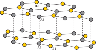
Figure 1: [color online] Lattice structure of the graphene bilayer. The A (B) sublattices are indicated by the darker (lighter) spheres and the planes are labeled by 1 and 2.

II.2 Bilayer graphene

Since the system is 2D only the relative position of the atoms projected on to the $x$-$y$-plane enters into the model. The projected position of the different atoms are shown in Fig. 2 together with the BZ.

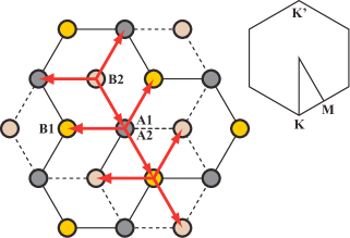
Figure 2: [color online] The real space lattice structure of the graphene bilayer projected onto the $x$-$y$ plane showing the relative positions of the different sublattices. The upper right corner shows the BZ of the graphene bilayer including the labeling of the high symmetry points.

Since the A atoms are sitting right on top of each other in the lattice, the hopping term between the $\text{A}1$ and $\text{A}2$ atoms are local in real space and hence a constant that we denote by $t_{\perp}$ in momentum space. Referring back to Section II.1 we note that the hopping $\text{B}1\rightarrow\text{A}1$ [$\text{A}1\rightarrow\text{B}1$] gives rise to the factor $\zeta({\bf k})$ [$\zeta^{*}({\bf k})$], with $\zeta({\bf k})$ defined in Eq. (4). Since the geometrical role of the A and B atoms are interchanged between plane 1 and plane 2 we immediately find that in Fourier space the hopping $\text{A}2\rightarrow\text{B}2$ [$\text{B}2\rightarrow\text{A}2$] gives rise to the factor $\zeta({\bf k})$ [$\zeta^{*}({\bf k})$]. Furthermore, the direction in the hopping $\text{B}1\rightarrow\text{B}2$ (projected on to the $x$-$y$ plane) is opposite to that of hopping $\text{B}1\rightarrow\text{A}1$. Thus we associate a factor $v_{3}\zeta^{*}({\bf k})$ to the hopping $\text{B}1\rightarrow\text{B}2$, where the factor $v_{3}=\gamma_{3}/\gamma_{0}$ is needed because the hopping energy is $\gamma_{3}$ instead of $\gamma_{0}=t$. Similarly, the direction of hopping $\text{B}1\rightarrow\text{A}2$ (projected on to the $x$-$y$ plane) is the same as $\text{B}1\rightarrow\text{A}1$ and therefore the term $-v_{4}\zeta({\bf k})$ goes with the hopping $\text{B}1\rightarrow\text{A}2$. The minus sign in front of $v_{4}$ follows from the conventional definition of $\gamma_{4}$ in graphite, as are discussed below. Continuing to fill in all the entries of the matrix the full tight-binding Hamiltonian in the graphene bilayer becomes:

$$\mathcal{H}_{\text{t.b.}}({\bf k})=\begin{pmatrix}V/2+\Delta&\zeta&t_{\perp}&-v_{4}\zeta^{*}\\ \zeta^{*}&V/2&-v_{4}\zeta^{*}&v_{3}\zeta\\ t_{\perp}&-v_{4}\zeta&-V/2+\Delta&\zeta^{*}\\ -v_{4}\zeta&v_{3}\zeta^{*}&\zeta&-V/2\end{pmatrix},$$ (5)

where the spinor is $\Psi^{{\dagger}}_{{\bf k}}=\bigl{(}c_{\text{A}1,{\bf k}}^{{\dagger}},\,c_{\text{B}1,{\bf k}}^{{\dagger}},\,c_{\text{A}2,{\bf k}}^{{\dagger}},\,c_{\text{B}2,{\bf k}}^{{\dagger}}\bigr{)}$. Here we have also introduced the conventional (from graphite) $\Delta$ that parametrizes the difference in energy between A and B atoms. In addition we included the parameter $V$ which gives different values of the potential energy in the two planes, such a term is generally allowed by symmetry and is generated by an electric field that is perpendicular to the two layers. The system with $V\neq 0$ is called the biased graphene bilayer and has a gap in the spectrum, in contrast the spectrum is gapless if $V=0$.

It is also possible to include further hoppings into the tight-binding picture, this was done for graphite by Johnson and Dresselhaus.Johnson and Dresselhaus (1973) The inclusion of such terms is necessary if one wants an accurate description of the bands throughout the whole BZ. If we expand the expression in Eq. (5) close to the K point in the BZ we obtain the matrix:

$$\mathcal{H}_{0}({\bf p})=\begin{pmatrix}V/2+\Delta&\sigma&t_{\perp}&-v_{4}\,\sigma^{*}\\ \sigma^{*}&V/2&-v_{4}\sigma^{*}&v_{3}\sigma\\ t_{\perp}&-v_{4}\sigma&-V/2+\Delta&\sigma^{*}\\ -v_{4}\sigma&v_{3}\sigma^{*}&\sigma&-V/2\end{pmatrix},$$ (6)

where $\sigma$ was introduced after Eq. (4).

The typical behavior of the bands obtained from Eq. (6) is shown in Fig. 3. Two of the bands are moved away from the Dirac point by an energy that is approximately given by the interplane hopping term $t_{\perp}$ for $V\ll t_{\perp}$. In the figure we have taken $V\neq 0$; but for $V=0$ there is no gap for the two bands closest to zero energy (i.e. the Dirac point).

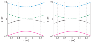
Figure 3: [color online] Band dispersions near the K points in the bilayer along the direction $\alpha=0$, with $V=50\,\text{meV}$ and $v_{\rm F}=1$. Left: bands obtained from the full model in Eq. (6) with $t_{\perp}=0.35\,\text{eV}$, $v_{3}=0.1$ and $v_{4}=0.05$; Right: bands obtained from the simplified model in Eq. (10).

II.3 The Slonsczewki-Weiss-McClure (SWM) model

First we make the observation that the graphene bilayer in the A-B stacking is just the unit cell of graphite that we depict in Fig. 1. Therefore, if the two planes are equivalent much of the symmetry analysis of graphite is also valid for the graphene bilayer. Thus we could alternatively use the SWM for graphite with the proper identification of the parameters. The SWM model for graphite,McClure (1957); Slonczewski and Weiss (1958) is usually written as

$$\mathcal{H}_{\text{SWMC}}=\begin{pmatrix}E_{1}&0&H_{13}&H_{13}^{*}\\ 0&E_{2}&H_{23}&-H_{23}^{*}\\ H_{13}^{*}&H_{23}^{*}&E_{3}&H_{33}\\ H_{13}&-H_{23}&H_{33}^{*}&E_{3}\end{pmatrix},$$ (7)

where

$$E_{1} = \Delta+\gamma_{1}\Gamma+\frac{1}{2}\gamma_{5}\Gamma^{2},$$ (8a)

$$E_{2} = \Delta-\gamma_{1}\Gamma+\frac{1}{2}\gamma_{5}\Gamma^{2},$$ (8b)

$$E_{3} = \frac{1}{2}\gamma_{2}\Gamma^{2},$$ (8c)

$$H_{13} = \frac{1}{\sqrt{2}}(-\gamma_{0}+\gamma_{4}\Gamma)e^{i\alpha}\zeta,$$ (8d)

$$H_{23} = \frac{1}{\sqrt{2}}(\gamma_{0}+\gamma_{4}\Gamma)e^{i\alpha}\zeta,$$ (8e)

$$H_{33} = \gamma_{3}\Gamma e^{i\alpha}\zeta.$$ (8f)

Here $\zeta=3ak/2$, and $\Gamma=2\cos(k_{\perp}d)$, with $d\approx 3.7\,\text{\AA}$ being the interplane distance. Typical values of the parameters from the graphite literature are shown in Table 1.

$\gamma_{0}$	$\gamma_{1}$	$\gamma_{2}$	$\gamma_{3}$	$\gamma_{4}$	$\gamma_{5}$	$\gamma_{6}=\Delta$	$\epsilon_{\text{F}}$
3.16	0.39	-0.02	0.315	0.044	0.038	0.008	-.024
3.12	0.377	-0.020	0.29	0.120	0.0125	0.004	-.0206

Table 1: Values of the SWM parameters for the band structure of graphite. Upper row from Ref. [Brandt et al., 1988] and lower row from Ref. [Chung, 2002].

It is straightforward to show that by identifying $\gamma_{1}=t_{\perp}$ and taking $\gamma_{2}=\gamma_{5}=0$, $\Gamma=1$ and $V=0$ the matrices in Eq. (6) and Eq. (7) are equivalent up to a unitary transformation. Hence they give rise to identical eigenvalues and band structures. This completes the correspondence between the tight-binding model and the SWM model (see also Refs. [Johnson and Dresselhaus, 1973; Partoens and Peeters, 2006] for a discussion on the connection between the tight-binding parameters and those of SWM.)

The accepted parameters from the graphite literature results in electrons near the K point [$k_{\perp}=0$] and holes near the H point [$k_{\perp}=\pi/(2d)$] in the BZ as sketched in Fig. 4. These electron and hole pockets are mainly generated by the coupling $\gamma_{2}$ that in the tight-binding model corresponds to a hopping between the B-atoms of next-nearest planes. Note that this process involves a hopping of a distance as large as $\sim 7\,\text{\AA}$.

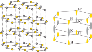
Figure 4: [color online] Left: graphite lattice; Right: three-dimensional BZ with the symmetry points K and H indicated. The accepted parameters for graphite results in electron pockets near the K points and hole pockets near the H points as sketched in the figure.

Finally, it is interesting to note that at the H-point in the BZ, $\Gamma=0$, and therefore the two planes “decouple” at this point. Furthermore, if one neglects $\Delta$ the spectrum is that of massless Dirac fermions just like in the case of graphene. Note that in graphite A and B atoms are different however, and that the term parametrized by $\Delta$, that breaks sublattice symmetry in each plane, opens a gap in the spectrum leading to massive Dirac fermions at the H-point. Since the value of $\Delta$ in the literature is quite small, the almost linear massless behavior should be observed by experimental probes that are not sensitive to this small energy scale.

The values of the parameters used in the graphite literature are consistent with a large number of experiments. The most accurate ones are various magneto-transport measurements discussed in Ref. [Brandt et al., 1988]. More recently, angle-resolved photo-emission spectroscopy (ARPES) was used to directly visualize the dispersion of massless Dirac quasi-particles near the H point and massive quasi-particles near the K point in the BZ.Zhou et al. (2006a, b); Ohta et al. (2006)

The band structure of graphite has been calculated and recalculated many times over the years, a recent reference is Ref. [Charlier et al., 1991]. It is also worth to mention that because of the (relatively) large contribution of the non-local van der Waals interaction to the interaction between the layers in graphite, the usual local density approximation or semilocal density approximation schemes are off by an order of magnitude when the binding energy of the planes are calculated and compared with experiments. For a discussion of this topic and a possible remedy, see Ref. [Rydberg et al., 2003].

III Simplified electronic band models

In this section we introduce three simplified models that we employ for most of the calculations in this paper. We also show how to obtain an effective two-band model that is sometimes useful.

III.1 Unbiased bilayer

For the unbiased bilayer, a minimal model includes only the nearest neighbor hopping energies within the planes and the interplane hopping term between A atoms; this leads to a Hamiltonian matrix of the form:

$$\mathcal{H}_{B}({\bf k})=\begin{pmatrix}0&ke^{i\phi({\bf k})}&t_{\perp}&0\\ ke^{-i\phi({\bf k})}&0&0&0\\ t_{\perp}&0&0&ke^{-i\phi({\bf k})}\\ 0&0&ke^{i\phi({\bf k})}&0\end{pmatrix},$$ (9)

near the K point in the BZ. Here we write $k_{x}+ik_{y}=ke^{i\phi({\bf k})}$, where $k=\sqrt{k_{x}^{2}+k_{y}^{2}}$ and $\phi({\bf k})$ is the appropriate angle. Note that the absolute value of the angle can be changed by a gauge transformation into a phase of the wave functions on the B sublattices. This reflects the rotational symmetry of the model. If one includes the “trigonal distortion” term parametrized by $\gamma_{3}$ the rotational symmetry is broken and it is necessary to keep track of the absolute value of the angle. From now on in this paper, we most often use units such that $v_{\rm F}=1$ for simplicity.

This Hamiltonian has the advantage that it allows for relatively simple calculations. Some of the fine details of the physics might not be accurate but it works as a minimal model and capture most of the important physics. It is important to know the qualitative nature of the terms that are neglected in this approximation, this is discussed later in this section. It is also an interesting toy model as it allows for (approximately) “chiral” particles with mass (i.e., a parabolic spectrum) at low energies.McCann and Fal’ko (2006)

III.2 Biased graphene bilayer

For the biased bilayer, a minimal model employs Eq. (9) augmented with the bias potential $V$:

$$\mathcal{H}_{BB}({\bf k})=\begin{pmatrix}V/2&ke^{i\phi({\bf k})}&t_{\perp}&0\\ ke^{-i\phi({\bf k})}&V/2&0&0\\ t_{\perp}&0&-V/2&ke^{-i\phi({\bf k})}\\ 0&0&ke^{i\phi({\bf k})}&-V/2\end{pmatrix}.$$ (10)

This model was introduced in Refs.  [Guinea et al., 2006; McCann, 2006]. It correctly captures the formation of an electronic gap of size $\sim V$ at the K point and the overall features of the bands as can be seen in Fig. 3. Nevertheless, the fine details of the bands close to the band edge are not captured correctly in this simple model; this fact is illustrated in Figs. 5-6. In particular the simple model is cylindrically symmetric; whereas the ”trigonal distortion” breaks this symmetry. Thus the inclusion of $v_{3}$ results in a ”trihorn” structure for small values of $V$ and a weaker modulation of the band edge for larger values of $V$ as illustrated in Fig. 5.

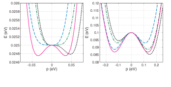
Figure 5: [color online] Band dispersions near the band edge (note the energy scale) in the biased graphene bilayer. Left: $V=50\,\text{meV}$, Right: $V=200\,\text{meV}$. The solid line is the simplified model in Eq. (10) that is cylindrically symmetric. The other lines are along different directions in the BZ for the full model in Eq. (6): $\alpha=0$ (dotted), $\alpha=\pi/9$ (dash-dotted), and $\alpha=2\pi/9$ (dashed). The parameters are the same as in Fig. 3

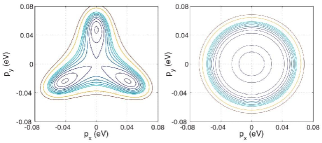
Figure 6: [color online] Contour plots of the band dispersions near the band edge in the biased graphene bilayer for $V=50\,\text{meV}$. Left: full model in Eq. (6), Right: simplified model in Eq. (10). The parameters are the same as in Fig. 3

III.3 Multilayer graphene

In the graphene multilayer, a minimal model for the bands is again given by Eq. (9) with the understanding that the momentum label also includes the perpendicular direction: ${\bf k}\rightarrow({\bf k}_{\parallel},k_{\perp})$. The only change is that we must make the substitution $t_{\perp}\rightarrow 2t_{\perp}\cos(k_{\perp}d)$ everywhere. Note that this is exactly the $\Gamma$-factor appearing in the SWM model discussed in Section II.3. In the following we often use units such that the interplane distance $d$ is set to $1$, then – since the unit cell holds two layers – the allowed values of $k_{\perp}$ lies in the interval $[-\pi/2,\pi/2]$. We note that this band model was used already in the seminal paper by Wallace as a simple model for graphite.Wallace (1947) More recent works on the band structure of few-layer graphene systems include Refs. Latil and Henrard, 2006; Partoens and Peeters, 2006; Guinea et al., 2006; Koshino and Ando, 2007; Nakamura and Hirasawa, .

III.4 Approximate effective two-band models

There are two main reasons for constructing approximate two-band models. Firstly, on physical grounds the high-energy bands (far away from the Dirac point) should not be very important for the low-energy properties of the system. Secondly, it is sometimes easier to work with $2\times 2$ instead of $4\times 4$ matrices. Nonetheless, it is not always a simplification to use the 2-band model when one is studying inhomogeneous systems as it generally leads to two coupled second order differential equations whereas the 4-band model involves four coupled linear differential equations. The matching of the wave functions in the 2-band case then involves both the continuity of the wave function and its derivative whereas in the 4-band model only continuity of the wave function is necessary. We note that the two-band description of the problem is only valid as long the electronic density is low enough, that is, when the Fermi energy is much smaller than $t_{\perp}$. At intermediate to high densities a 4-band model is required in order to obtain the correct physical properties.Kusminskiy et al. (2007)

In this section, we derive the low-energy effective model by doing degenerate second order perturbation theory. The quality of the expansion is good as long as $v_{\rm F}p\ll t_{\perp}\approx 0.35\,\text{eV}$. We first present the general expression for the second-order $2\times 2$ effective Hamiltonian, thereafter various simplified forms are introduced. Analyses similar to the one here were previously described in Refs. [McCann and Fal’ko, 2006; Nilsson et al., 2006b].

First we introduce the projector matrices $\mathcal{P}_{0}=\text{Diag}[0,\,1,\,0,\,1]$ ($\mathcal{P}_{1}=\text{Diag}[1,\,0,\,1,\,0]$) that projects onto (out of) the low-energy subspace of the B atoms. Then we split the Hamiltonian in Eq. (6) according to: $\mathcal{H}_{0}=\mathcal{K}_{0}+\mathcal{K}_{1}+\mathcal{K}_{2}$, with

$$\mathcal{K}_{0}=\begin{pmatrix}\Delta+V/2&0&t_{\perp}&0\\ 0&V/2&0&0\\ t_{\perp}&0&\Delta-V/2&0\\ 0&0&0&-V/2\end{pmatrix},$$ (11)

$$\mathcal{K}_{1}=v_{\rm F}\begin{pmatrix}0&pe^{i\phi}&0&-v_{4}pe^{-i\phi}\\ pe^{-i\phi}&0&-v_{4}pe^{-i\phi}&0\\ 0&-v_{4}pe^{i\phi}&0&pe^{-i\phi}\\ -v_{4}pe^{i\phi}&0&pe^{i\phi}&0\end{pmatrix},$$ (12)

$$\mathcal{K}_{2}=v_{\rm F}\begin{pmatrix}0&0&0&0\\ 0&0&0&v_{3}pe^{i\phi}\\ 0&0&0&0\\ 0&v_{3}pe^{-i\phi}&0&0\end{pmatrix}.$$ (13)

Introducing the vectors $\bigl{\{}|l\rangle\bigr{\}}$ that to zeroth order only have components in the low energy subspace (i.e., $\mathcal{P}_{1}|l^{(0)}\rangle=0$) and following the standard procedure (see e.g., Ref. [Sakurai, 1994]) for degenerate perturbation theory we arrive at:

$$\langle l|\mathcal{P}_{0}\,\mathcal{H}_{0}\,\mathcal{P}_{0}|l^{\prime}\rangle\approx\langle l|\mathcal{P}_{0}\bigl{[}\mathcal{K}_{0}+\lambda^{2}\mathcal{K}_{2}\bigr{]}\mathcal{P}_{0}|l^{\prime}\rangle\\ +\lambda^{2}\langle l|\mathcal{P}_{0}\mathcal{K}_{1}\mathcal{P}_{1}\frac{1}{\hat{E}-\mathcal{K}_{0}}\mathcal{P}_{1}\mathcal{K}_{1}\mathcal{P}_{0}|l^{\prime}\rangle,$$ (14)

where we explicitly assume that $\mathcal{K}_{2}$ is of the same order as $\mathcal{K}_{1}^{2}/\mathcal{K}_{0}$. This expression is correct to second order in $\lambda$. Note that we are doing second order perturbation theory for all of the components of the $2\times 2$-matrix in the low-energy subspace. Working to first order in $\lambda^{2}$ (and then setting $\lambda=1$) one obtains for this matrix (taking $v_{\rm F}=1$ for brevity):

$$\mathcal{K}_{\text{low}}=\begin{pmatrix}V/2&v_{3}pe^{i\phi}\\ v_{3}pe^{-i\phi}&-V/2\end{pmatrix}\\ +\begin{pmatrix}\frac{-V+2t_{\perp}v_{4}+\Delta(1+v_{4}^{2})}{t_{\perp}^{2}-\Delta(\Delta-V)}&-\frac{t_{\perp}(1+v_{4}^{2})+2v_{4}\Delta}{t_{\perp}^{2}+V^{2}/4-\Delta^{2}}e^{-2i\phi}\\ -\frac{t_{\perp}(1+v_{4}^{2})+2v_{4}\Delta}{t_{\perp}^{2}+V^{2}/4-\Delta^{2}}e^{2i\phi}&\frac{V+2t_{\perp}v_{4}+\Delta(1+v_{4}^{2})}{t_{\perp}^{2}-\Delta(\Delta+V)}\end{pmatrix}p^{2}.$$ (15)

Taking $\Delta=0$ leads to an even simpler expression, in particular the effective spectrum becomes:

$$E_{\text{low},\pm}\approx\frac{2v_{4}p^{2}}{t_{\perp}}\pm\sqrt{\Bigl{[}1-\frac{2p^{2}}{t_{\perp}^{2}}\Bigr{]}^{2}\frac{V^{2}}{4}+(v_{3}p)^{2}+\Bigl{\{}\frac{p^{2}\bigl{[}t_{\perp}(1+v_{4}^{2})\bigr{]}}{t_{\perp}^{2}+V^{2}/4}\Bigr{\}}^{2}-\frac{2v_{3}p^{3}\bigl{[}t_{\perp}(1+v_{4}^{2})\bigr{]}}{t_{\perp}^{2}+V^{2}/4}\cos(3\phi)}.$$ (16)

That this approximation to the bands is excellent near the band edge for small values of the bias $V$ is illustrated in Fig. 7. For larger values of the bias the agreement is less accurate because the assumption of smallness of certain terms in the perturbation expansion is no longer valid.

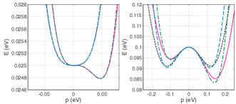
Figure 7: [color online] Band dispersions near the band edge in the biased graphene bilayer along two directions in the BZ. Left: $V=50\,\text{meV}$, Right: $V=200\,\text{meV}$. The solid (dash-dotted) line is the effective model in Eq. (16) along $\alpha=0$ ($\alpha=\pi/6$). The dotted (dashed) line is the full model in Eq. (6) along $\alpha=0$ ($\alpha=\pi/6$). The parameters are the same as in Fig. 3. For $V=50\,\text{meV}$ the different curves are almost not discernible.

IV Green’s function in the graphene bilayer

As discussed in Section III we use the minimal model Hamiltonian in Eq. (9). We note that the phases $\phi\equiv\phi({\bf k})$ can be gauged away by an application of a unitary transformation defined by the matrix

$$\mathcal{M}_{1}({\bf k})=\begin{pmatrix}1&0&0&0\\ 0&e^{-i\phi({\bf k})}&0&0\\ 0&0&1&0\\ 0&0&0&e^{i\phi({\bf k})}\end{pmatrix}.$$ (17)

It is also easy to compute the energy eigenvalues that are given by $t_{\perp}/2\pm\sqrt{t_{\perp}^{2}/4+k^{2}}$ and $-t_{\perp}/2\pm\sqrt{t_{\perp}^{2}/4+k^{2}}$. Before we solve for the Green’s functions it is convenient to allow for a local frequency dependent self-energy in the problem. In the general case the self-energies on all of the inequivalent sites in the problem are allowed to be different, and we explicitly introduce the matrix

$$\mathcal{H}_{\Sigma}(\omega)=\begin{pmatrix}\Sigma_{\text{A}1}(\omega)&0&0&0\\ 0&\Sigma_{\text{B}1}(\omega)&0&0\\ 0&0&\Sigma_{\text{A}2}(\omega)&0\\ 0&0&0&\Sigma_{\text{B}2}(\omega)\end{pmatrix},$$ (18)

to describe this. The Green’s function matrix is then given by the equation

$${\rm G}^{-1}(\omega,{\bf k})=\omega-\mathcal{H}_{0}({\bf k})-\mathcal{H}_{\Sigma}(\omega).$$ (19)

In the case of the unbiased bilayer the A (B) sites in both of the layers are equivalent and we only need two self-energies: $\Sigma_{\text{A}}(\omega)$ and $\Sigma_{\text{B}}(\omega)$ which are local but we allow for a frequency ($\omega$) dependence. In this case the matrix inversion is simple since it factorizes into two $2\times 2$ matrices. An explicit form is given by

$${\rm G}(\omega,{\bf k})=\mathcal{M}_{1}({\bf k})\begin{pmatrix}{\rm g^{D}}(\omega,k)&{\rm g^{ND}}(\omega,k)\\ {\rm g^{ND}}(\omega,k)&{\rm g^{D}}(\omega,k)\end{pmatrix}\mathcal{M}_{1}^{{\dagger}}({\bf k}),$$ (20)

where $k=|{\bf k}|$. Here D (ND) stands for diagonal (non-diagonal) in the layer index. The components of the g-matrices are given by

$${\rm g_{AA}^{D,ND}} = \frac{\omega-\Sigma_{\text{B}}}{2D_{-}}\pm\frac{\omega-\Sigma_{\text{B}}}{2D_{+}},$$ (21a)

$${\rm g_{BB}^{D,ND}} = \frac{\omega-t_{\perp}-\Sigma_{\text{A}}}{2D_{-}}\pm\frac{\omega+t_{\perp}-\Sigma_{\text{A}}}{2D_{+}},$$ (21b)

$${\rm g_{AB}^{D,ND}} = \frac{k}{2D_{-}}\pm\frac{k}{2D_{+}},$$ (21c)

where

$$D_{\pm}(\omega,p)=\bigl{[}\omega\pm t_{\perp}-\Sigma_{\text{A}}(\omega)\bigl{]}\bigl{[}\omega-\Sigma_{\text{B}}(\omega)\bigr{]}-k^{2}.$$ (22)

Note that we often suppress the momentum and frequency dependence in the following when no confusion arises. We will come back to the biased case in Section XV.

V Impurity scattering: t-matrix and coherent potential approximation

We are interested in the influence of disorder in the bilayer. To model the impurities we use the standard t-matrix approach and the Coherent Potential Approximation (CPA). The effect of repeated scattering from a single impurity can be encoded in a self-energy which can be computed from:Jones and March (1985)

$$\Sigma_{j}=V_{j}+V_{j}N\overline{{\rm G}}V_{j}+V_{j}N\overline{{\rm G}}V_{j}N\overline{{\rm G}}V_{j}+\ldots\\ =V_{j}\bigl{[}1-N\overline{{\rm G}}V_{j}]^{-1}.$$ (23)

Here $V_{j}$ is a matrix that encodes both the strength and the lattice site of the impurity in question. For example, an impurity on an A1 lattice site of strength $U$ at the origin is encoded in Fourier space by the matrix

$$V_{1}=\frac{U}{N}\begin{pmatrix}1&0&0&0\\ 0&0&0&0\\ 0&0&0&0\\ 0&0&0&0\end{pmatrix},$$ (24)

implying that the potential is located only on a single site. We have also introduced the quantity:

$$\overline{{\rm G}}_{\alpha j}(\omega)=\frac{1}{N}\sum_{{\bf k}}{\rm G}_{\alpha j\alpha j}(\omega,{\bf k})\\ \approx\frac{1}{\Lambda^{2}}\int_{0}^{\Lambda^{2}}d(k^{2})\int\frac{d\phi}{2\pi}\,{\rm G}_{\alpha j\alpha j}(\omega,{\bf k}),$$ (25)

which is the local propagator at the impurity site; and in the second step the ${\bf k}$-sum is to be taken over the whole BZ. The last line is an approximate expression that is obtained by expanding the propagator close to the K points and taking the continuum limit with the introducing of the cutoff $\Lambda$. We estimate the cutoff by a Debye approximation that conserves the number of states in the BZ. Then $\Lambda\approx 7\text{eV}$ and in units of the cutoff we have $t_{\perp}\approx 0.05$ (taking $t_{\perp}\approx 0.35\,\text{eV}$). Due to the special form of the propagator and the impurity potential the self-energy we get from this is diagonal. The result for site dilution (or vacancies) is obtained by taking the limit $U\rightarrow\infty$, so that the electrons are not allowed to enter the site in question. We also introduce a finite density $n_{\rm i}$ of impurities in the system. To leading order in the impurity concentration the equations for the self-energies then become:

$$\frac{n_{i}}{\Sigma_{\text{A}}} = -\overline{{\rm G}}_{\text{A}},$$ (26a)

$$\frac{n_{i}}{\Sigma_{\text{B}}} = -\overline{{\rm G}}_{\text{B}}.$$ (26b)

The explicit form of the propagators in Eq. (21) makes it easy to compute the $\overline{\text{G}}$’s. The t-matrix result for the self-energies is obtained by using the bare propagators on the right hand side of Eq. (26). In the CPA one assumes that the electrons are moving in an effective medium with recovered translational invariance which in this case is characterized by the local self-energies. To determine what the medium is, one must solve the equations self-consistently with the full propagators on the right hand side of Eq. (26). Because of the simple form of the propagators this is a simple numerical task in the model we are using. To simplify the equations further we assume that $\Lambda\gg\omega,t_{\perp},\Sigma_{\text{A}},\Sigma_{\text{B}}$. This is a physical assumption since when the self-energies becomes of the order of the cutoff the effective theory breaks down. The self-consistent equations then reads:

$$\bigl{[}\frac{\Sigma_{\text{A}}}{n_{i}}\bigr{]}^{-1}=-\overline{{\rm G}}_{\text{A}}=\\ \frac{\omega-\Sigma_{\text{B}}}{2\Lambda^{2}}\sum_{\alpha=\pm}\log\Bigl{[}\frac{\Lambda^{2}}{-(\omega+\alpha t_{\perp}-\Sigma_{\text{A}})(\omega-\Sigma_{\text{B}})}\Bigr{]},$$ (27a)

$$\bigl{[}\frac{\Sigma_{\text{B}}}{n_{i}}\bigr{]}^{-1}=-\overline{{\rm G}}_{\text{B}}\\ =\frac{\omega-\Sigma_{\text{A}}}{2\Lambda^{2}}\sum_{\alpha=\pm}\log\Bigl{[}\frac{\Lambda^{2}}{-(\omega-\alpha t_{\perp}-\Sigma_{\text{A}})(\omega-\Sigma_{\text{B}})}\Bigr{]}\\ +\frac{t_{\perp}}{2\Lambda^{2}}\log\Bigl{[}\frac{-(\omega-t_{\perp}-\Sigma_{\text{A}})(\omega-\Sigma_{\text{B}})}{-(\omega+t_{\perp}-\Sigma_{\text{A}})(\omega-\Sigma_{\text{B}})}\Bigr{]}.$$ (27b)

This includes inter-valley scattering in the intermediate states. It is easy to obtain the non-disordered density of states from these equations by taking $\Sigma_{\text{A}}=\Sigma_{\text{B}}=0$ and $\omega\rightarrow\omega+i\delta$ (here $\delta$ is a positive infinitesimal) resulting in:

$$\rho_{\text{A}}^{0}(\omega)=-\frac{1}{\pi}\operatorname{Im}\overline{{\rm G}}_{\text{A}}=\frac{|\omega|}{2\Lambda^{2}}\bigl{[}1+\Theta(|\omega|-t_{\perp})\bigr{]},$$ (28a)

$$\rho_{\text{B}}^{0}(\omega)=-\frac{1}{\pi}\operatorname{Im}\overline{{\rm G}}_{\text{B}}\\ =\frac{|\omega|}{2\Lambda^{2}}\bigl{[}1+\Theta(|\omega|-t_{\perp})\bigr{]}+\frac{t_{\perp}}{2\Lambda^{2}}\bigl{[}1-\Theta(|\omega|-t_{\perp})\bigr{]}.$$ (28b)

Observe in particular that the density of states on the A sublattice goes to zero in the limit of zero frequency, this fact is responsible for much of the unconventional physics in the graphene bilayer. In contrast the density of states on the B sublattice is finite at $\omega=0$. We discuss how this result is changed with disorder and the solution of Eq. (27) in the following.

V.1 Zero frequency limit

One interesting feature of the CPA equations in Eq. (27) is that it is easy to see that they do not allow for a finite $\Sigma_{\text{A}}$ in the limit of $\omega\rightarrow 0$. Since by setting $\omega=0$ the last term in Eq. (27b) must vanish, and this is not possible for finite values of $\Sigma_{\text{A}}$. Then one also must have that $\Sigma_{\text{B}}\rightarrow 0$ there. This implies that the density of states on sublattice A is still zero even within the CPA in the limit $\omega\rightarrow 0$. More explicitly, by defining $\Sigma_{\text{A}}\Sigma_{\text{B}}=-\xi\Lambda^{2}$ one can show (assuming $\Sigma_{\text{A}}\gg t_{\perp}$ and $\Sigma_{\text{B}}\gg\omega$) that $\Sigma_{\text{A}}$ and $\Sigma_{\text{B}}$ are given asymptotically by:

$$\Sigma_{\text{A}} = \Bigl{(}\frac{t_{\perp}^{2}\xi^{2}\Lambda^{2}}{n_{i}\omega}\Bigr{)}^{1/3}e^{-i\pi/3},$$ (29a)

$$\Sigma_{\text{B}} = \Bigl{(}\frac{n_{i}\Lambda^{4}\xi\omega}{t_{\perp}^{2}}\Bigr{)}^{1/3}e^{-i2\pi/3},$$ (29b)

and $\xi$ satisfies

$$n_{i}=\xi\log(1/\xi).$$ (30)

Notice that $\sqrt{\xi}\Lambda\sim\sqrt{n_{i}}\Lambda$ is exactly the energy scale that is generated by disorder of the same kind in the single layer case.Peres et al. (2006) We have checked that the expressions in Eq. (29) seem to agree with the numerical calculations in the small frequency limit, and the frequency range in which they holds grows with increasing $n_{i}$.

V.2 Uncompensated impurity densities

The divergence of the self-energy $\Sigma_{\text{A}}$ on the A sublattice in the CPA in the above is due to the fact that there is a perfect compensation between the number of impurities on the two sublattices: $n_{{\rm i},\text{A}}=n_{{\rm i},\text{B}}$. For the more general case where $n_{{\rm i},\text{A}}\neq n_{{\rm i},\text{B}}$ the divergence is not present so that $\Sigma_{\text{A}}$ may become finite at $\omega=0$. To make comparison with other work on the graphene bilayer it is fruitful to consider another extreme limit where only the B sites are affected by the disorder. Explicitly this means that we take $n_{{\rm i},\text{A}}=0$ and $n_{{\rm i},\text{B}}\neq 0$. The generalization of the CPA equations in Eq. (27) for this case then immediately imply that $\Sigma_{\text{A}}(\omega)\equiv 0$. In the limit of $\omega\rightarrow 0$, $\Sigma_{\text{B}}$ is finite, purely imaginary, and given by:

$$\Sigma_{\text{B}}(\omega=0)=-i\frac{2\Lambda^{2}}{\pi t_{\perp}}n_{{\rm i},\text{B}}\equiv-i\Gamma.$$ (31)

V.3 Born scattering

Another often studied limit is the one of weak impurities, in particular Koshino and Ando have studied electron transport in the graphene bilayer in this approximation.Koshino and Ando (2006) This is the Born limit and it can be studied using perturbation theory in the strength of the impurities $U$. The leading non-trivial contribution to the self-energies is given by the contribution to second order:

$$\Sigma_{\text{A}} = n_{\rm i}U\overline{{\rm G}}_{\text{A}}U,$$ (32a)

$$\Sigma_{\text{B}} = n_{\rm i}U\overline{{\rm G}}_{\text{B}}U.$$ (32b)

If one substitutes the bare propagators on the right hand side one finds $\Sigma_{\text{A}}=0$ and $\Sigma_{\text{B}}=-i\pi n_{\rm i}t_{\perp}(U/\Lambda)^{2}/2$ at the Dirac point. Thus, to leading order Born scattering is formally equivalent to the previous case with vacancies on only sublattice B exactly at $\omega=0$. The frequency range for which the $\omega=0$ result is valid is different however.

V.4 Self-energy comparisons and the density of states

We compare the self-energies obtained from the t-matrix and the CPA. Within the t-matrix the self-energies are given by

$$\Sigma_{\text{A}} = \frac{n_{i}}{F_{\text{A}}^{0}+i\pi\rho_{\text{A}}^{0}(\omega)},$$ (33a)

$$\Sigma_{\text{B}} = \frac{n_{i}}{F_{\text{B}}^{0}+i\pi\rho_{\text{B}}^{0}(\omega)},$$ (33b)

where the $\rho^{0}$’s are given in Eq. (28) and

$$F_{\text{A}}^{0}\equiv-\operatorname{Re}\bigl{[}\,\overline{{\rm G}}^{0}_{\text{AA}}\,\bigr{]} = \frac{\omega}{2\Lambda^{2}}\log\Bigl{(}\frac{\Lambda^{4}}{\omega^{2}|\omega^{2}-t_{\perp}^{2}|}\Bigr{)},$$ (34a)

$$F_{\text{B}}^{0}\equiv-\operatorname{Re}\bigl{[}\,\overline{{\rm G}}^{0}_{\text{BB}}\,\bigr{]} = F_{\text{A}}^{0}+\frac{t_{\perp}}{2\Lambda^{2}}\log\Bigl{|}\frac{\omega-t_{\perp}}{\omega+t_{\perp}}\Bigr{|}.$$ (34b)

The results for the self-energies in the two different approximations are shown in Figs. 8 and 9. Note that at least on the scale of the figures the $\Sigma_{A}$ diverges as $\omega\rightarrow 0$ in the CPA, as discussed above. The solution to the self-consistent equations also does not converge very well when they are pushed close to the limit of $\omega\rightarrow 0$. The total DOS on the A-sublattice and B-sublattice is pictured in Fig. 10. Note in particular that the case of $n_{i}=.0001$ closely resemble the non-interacting case except for the new low-energy feature. A possible interpretation of the enhancement of the DOS on the B sublattice near $\omega=0$ is in terms of the “half-localized” states (meaning they do not decay fast enough to be normalizable at infinity) that have been studied for monolayer graphene.Pereira et al. (2006) Because these states have weight on only one sublattice (the opposite one of the vacancy) the construction in Ref. [Pereira et al., 2006] is valid also in the graphene bilayer when there is a vacancy on one of the A sublattices. For a discussion of the related problem of edge states in bilayer graphene see Ref. [Castro et al., ].

Figure 8: [color online] Self-energies within the t-matrix approximation in the bilayer as a function of the frequency $\omega$. Left: sublattice A; Right: sublattice B.

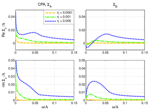
Figure 9: [color online] Self-energies within the CPA in the bilayer as a function of the frequency $\omega$. Left: sublattice A; Right: sublattice B.

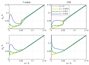
Figure 10: [color online] Local density of states $\rho$ on the different sublattices in the bilayer. Left: t-matrix; Right: CPA. Top: sublattice A; Bottom: sublattice B.

V.5 Spectral function

The electron spectral function $A({\bf k},\omega)$, which is observable in ARPES experiments, is defined by $A({\bf k},\omega)\equiv-\text{Trace}[\operatorname{Im}\,{\rm G}({\bf k},\omega)]/\pi$, so that in our case:

$$A({\bf k},\omega)=-\frac{2}{\pi}\Bigl{\{}\operatorname{Im}\bigl{[}{\rm G}_{\rm AA}^{\rm D}({\bf k},\omega)\bigl{]}+\operatorname{Im}\bigl{[}{\rm G}_{\rm BB}^{\rm D}({\bf k},\omega)\bigl{]}\Bigr{\}}.$$ (35)

The spectral function in the $k\times\omega$ plane, calculated within the CPA, is pictured in Fig. 11. As can be seen in the figures the low-energy branch becomes significantly blurred, especially for the higher impurity concentrations. Note also that the gap to the high-energy branch becomes slightly larger as the disorder value increases due to the fact that $\Sigma_{\text{A}}$ is not negligible there.

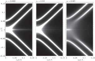
Figure 11: Intensity plot of the spectral function in the $k\times\omega$ plane (normalized by the cutoff) in the bilayer for different impurity concentrations in the CPA approximation. From left to right: $n_{i}=10^{-4}$, $10^{-3}$, $5\times 10^{-3}$.

Examples of the momentum distribution curves (MDC’s) and the energy distribution curves (EDC’s) in the disordered graphene bilayer are shown in Figs. 12 and 13. The evolution of the peaks from delta functions to broader peaks with increasing disorder is clear in the figure.

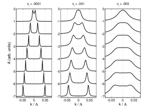
Figure 12: MDC’s in the graphene bilayer. The three panels are for different impurity concentrations and are calculated in the CPA. From the top the energy cuts are at the energies: .0005, .0055, .0105, .0155, .0205, .0255, and .0305 in units of the cutoff $\Lambda$. The curves are uniformly displaced for clarity.

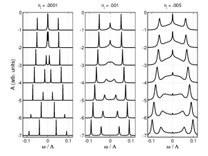
Figure 13: EDC’s in the graphene bilayer. The three panels are for different impurity concentrations and are calculated in the CPA. From the top the cuts are at fixed values of the in-plane momentum $k$: .0001, .01, .02, .03, .04, .05, and .06 in units of the cutoff $\Lambda$. The curves are uniformly displaced for clarity.

VI Green’s function and one-particle properties in multilayer graphene

We will use the extension of the bilayer model to the multilayer that we introduced in Section III.3. As discussed there we can immediately use the Hamiltonian in Eq. (9) with the understanding that the momentum label also includes the perpendicular direction: ${\bf k}\rightarrow({\bf k}_{\parallel},k_{\perp})$ and by substituting $t_{\perp}\rightarrow 2t_{\perp}\cos(k_{\perp}d)$ everywhere. In particular the Green’s function including the self-energies are again given by the expressions in Eq. (21) and Eq. (22) with the substitution $t_{\perp}\rightarrow 2t_{\perp}\cos(k_{\perp}d)$.

VI.1 Self-energies and the density of states

To get the CPA equations we must evaluate the local propagator $\overline{{\rm G}}$ that is given by the straightforward generalization of Eq. (25) to include an extra sum over $k_{\perp}$:

$$\overline{{\rm G}}(\omega)=\frac{1}{N}\sum_{{\bf k}_{\parallel}}\frac{1}{N_{c}}\sum_{k_{\perp}}{\rm G}(\omega).$$ (36)

Here $N_{c}$ is the number of unit cells in the perpendicular direction. This extra sum can be transformed into an integral using the relation $\frac{1}{N_{c}}\sum_{k_{\perp}}\rightarrow\int_{-\pi/2}^{\pi/2}\frac{dk_{\perp}}{\pi}$. It is possible to perform the integrals analytically as we explain in App. B. Using the integrals defined there ($I_{1}$ and $I_{2}$) we obtain for $\omega,\Sigma_{\text{A}},\Sigma_{\text{B}},t_{\perp}\ll\Lambda$

$$\frac{n_{i}}{\Sigma_{\text{A}}} = -\overline{\rm G}_{\rm AA}^{\rm D}=-\frac{\omega-\Sigma_{\text{B}}}{\Lambda^{2}}I_{1},$$ (37a)

$$\frac{n_{i}}{\Sigma_{\text{B}}} = -\overline{\rm G}_{\rm BB}^{\rm D}=-\frac{\omega-\Sigma_{\text{A}}}{\Lambda^{2}}I_{1}-\frac{1}{\Lambda^{2}}I_{2}.$$ (37b)

From these equations one can easily obtain the non-interacting density of states by considering the clean retarded case and take $\Sigma_{A}=\Sigma_{B}=0$ and $\omega\rightarrow\omega+i\delta$, from which we get:

$$\rho_{\text{A}}^{0}=\frac{|\omega|}{\pi\Lambda^{2}}\Bigl{[}\frac{\pi}{2}+\tan^{-1}(\frac{|\omega|}{\sqrt{4t_{\perp}^{2}-\omega^{2}}})\Bigr{]}\Theta(2t_{\perp}-|\omega|)\\ +\frac{|\omega|}{\Lambda^{2}}\Theta(|\omega|-2t_{\perp}),$$ (38a)

$$\rho_{\text{B}}^{0}=\rho_{\text{A}}^{0}+\frac{\sqrt{4t_{\perp}^{2}-\omega^{2}}}{\pi\Lambda^{2}}\Theta(2t_{\perp}-|\omega|).$$ (38b)

The equivalent expression were previously obtained in Ref. [Guinea et al., 2006] using a different method. The self-energy within the t-matrix is again given by the expression in Eq. (33), with the $\rho$’s given by the non-interacting density of states in Eq. (38). The F’s are obtained from the real parts of the non-interacting local propagators:

$$F_{\text{A}}^{0}=\frac{\omega}{\Lambda^{2}}\log\Bigl{(}\frac{\Lambda^{2}}{t_{\perp}|\omega|}\Bigr{)}\Theta(2t_{\perp}-|\omega|)\\ +\frac{\omega}{\Lambda^{2}}\log\Bigl{(}\frac{2\Lambda^{2}}{|\omega|(|\omega|+\sqrt{\omega^{2}-4t_{\perp}^{2}})}\Bigr{)}\Theta(|\omega|-2t_{\perp}),$$ (39a)

$$F_{\text{B}}^{0}=F_{\text{A}}^{0}-\frac{\omega}{\Lambda^{2}}+\operatorname{sign}(\omega)\frac{\sqrt{\omega^{2}-4t_{\perp}^{2}}}{\Lambda^{2}}\Theta(|\omega|-2t_{\perp}).$$ (39b)

The self-energies obtained within the t-matrix are shown in Fig. 14 while those obtained from the CPA are shown in Fig. 15. A comparison between the density of states in the different approximations is shown in Fig. 16. In general the curves are similar to the ones in the bilayer but somewhat smoother.

The behavior of the self-energies at the Dirac point in the multilayer are similar to the case of the bilayer treated in Section V.1, V.2 and V.3. We have more to say about this when we discuss the perpendicular transport in the multilayer in Section IX.1.

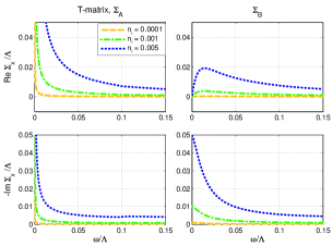
Figure 14: [color online] Self-energies within the t-matrix in the multilayer as a function of the frequency $\omega$. Left: sublattice A; Right: sublattice B.

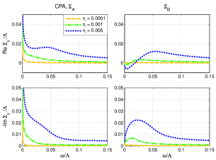
Figure 15: [color online] Self-energies within the CPA in the multilayer as a function of the frequency $\omega$. Left: sublattice A; Right: sublattice B.

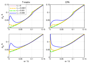
Figure 16: [color online] Local density of states $\rho$ on the different sublattices as a function of the frequency $\omega$ in the multilayer. Top: sublattice A; Bottom: sublattice B.

VI.2 Spectral function

The spectral function for the graphene multilayer is given by a generalization of Eq. (35):

$$A({\bf k}_{\parallel},k_{\perp},\omega)=-\frac{2}{\pi}\Bigl{\{}\operatorname{Im}\bigl{[}{\rm G}_{\rm AA}^{\rm D}(k_{\parallel},k_{\perp},\omega)\bigl{]}\\ +\operatorname{Im}\bigl{[}{\rm G}_{\rm BB}^{\rm D}(k_{\parallel},k_{\perp},\omega)\bigl{]}\Bigr{\}}.$$ (40)

Given the form of the Green’s function and the CPA self-energies it is straightforward to obtain this quantity. The spectral function is depicted in Fig. 17 for three values of the perpendicular momentum, since the model we use is electron-hole symmetric we only show the results for negative frequencies. We would like to stress that for a large part of the BZ the spectra are reminiscent of the bilayer spectra. At the edges of the BZ however, where $2t_{\perp}\cos(k_{\perp}d)=0$, the spectrum is that of massless Dirac fermions.

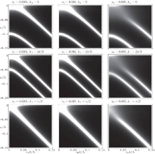
Figure 17: Intensity plot of the electron spectral function in the $k\times\omega$ plane for the multilayer for different disorder values and different values of $k_{\perp}$ in the CPA. From left to right: $n_{i}=10^{-4}$, $10^{-3}$, $5\times 10^{-3}$. From top to bottom: $k_{\perp}=0$, $\pi/(3d)$, $\pi/(2d)$.

Examples of the momentum distribution curves (MDC’s) and the energy distribution curves (EDC’s) in the disordered graphene multilayer are shown in Figs. 18 and 19 for two different values of $k_{\perp}$. The evolution of the peaks from delta functions to broader peaks with increasing disorder is clearly seen. One can also note that the influence of the impurities is more severe close to the H point of the BZ since the overlap of the peaks is larger there. The reason for this is that the particles there are dispersing linearly leading to peaks that are closer together than for particles with a parabolic dispersion.

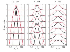
Figure 18: [color online] MDC’s in the graphene multilayer for two values of the perpendicular momentum: $k_{\perp}=0$ (i.e. at the K point, parabolic dispersion, dashed line) and $k_{\perp}=\pi/2$ (i.e. at the H point, linear dispersion, solid line). The three panels are for different values of the density of impurities in the CPA. From the top the energy cuts are at the energies: .0005, .0055, .0105, .0155, .0205, .0255, and .0305 in units of the cutoff $\Lambda$. The curves are uniformly displaced for clarity.

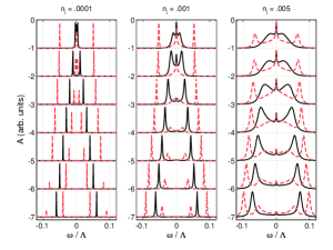
Figure 19: [color online] EDC’s in the graphene multilayer for two values of the perpendicular momentum: $k_{\perp}=\pi/3$ (i.e. between the K and H point, parabolic dispersion, dashed line) and $k_{\perp}=\pi/2$ (i.e. at the H point, linear dispersion, solid line). The three panels are for different values of the density of impurities in the CPA. From the top the cuts are at fixed values of the in-plane momentum $k_{||}$: .0001, .01, .02, .03, .04, .05, and .06 in units of the cutoff $\Lambda$. The curves are uniformly displaced for clarity.

VII Electron transport in bilayer and multilayer graphene

Having worked out the self-energies in the previous sections we now turn to linear response (Kubo formula) to study electron transport. We saw in Sections V and VI that the low-energy states are mainly residing on the B sublattice. Nevertheless, electron transport coming from nearest neighbor hopping must go over the A sublattice. This is particularly important for the case of perpendicular transport, since in the simple model that we are using, hopping comes exclusively from states with weight on the A sublattice.

This feature implies that although the total density of states at half-filling is finite, because the density of states on the A sublattice goes to zero as the Dirac point is approached, the in-plane and out-of-plane transport properties are unconventional. The main purpose of this section and the two following sections is to show how this comes about in detail through concrete calculations. We calculate conductivities (or optical response) parallel and perpendicular to the planes in both bilayer graphene and multilayer graphene. The resulting conductivities are very anisotropic and we find a universal nonzero minimum value for the in-plane DC conductivity as a function of the chemical potential.

VII.1 Conductivity formulas

To calculate the conductivity we use the Kubo formula.Mahan (2000) We only consider the homogeneous (${\bf q}=0$) response, but we investigate both the temperature dependence and the frequency dependence of the various conductivities.

The conductivity is computed from the Kubo formula:

$$\sigma(\omega)=\frac{1}{S\omega}\int_{0}^{\infty}dte^{i\omega t}\langle[J^{{\dagger}}(t),J(0)]\rangle=\frac{i}{\omega+i\delta}\Pi(\omega).$$ (41)

Here $S$ is the area of the system, $J$ is the current operator of interest, and $\Pi$ the appropriate current-current correlation function. A contribution to $\Pi$ from a term of the form $\langle[A(t),B(0)]\rangle$ where $A=\sum_{{\bf k}}\alpha({\bf k})a_{1{\bf k}}^{{\dagger}}a_{2{\bf k}}$ and $B=\sum_{{\bf k}}\beta({\bf k})b_{1{\bf k}}^{{\dagger}}b_{2{\bf k}}$ can be shown by the usual methods to give a contribution to the real part of the conductivity of the form:

$$\operatorname{Re}\bigl{[}\sigma(\omega)\bigr{]}=\frac{1}{S}\sum_{{\bf k}}\int\frac{d\epsilon}{\pi}\Bigl{[}-\frac{n_{\rm F}(\epsilon+\omega)-n_{\rm F}(\epsilon)}{\omega}\Bigr{]}\\ \times\operatorname{Im}\bigl{[}{\rm G}_{b2,a1}(\epsilon,{\bf k})\bigr{]}\operatorname{Im}\bigl{[}{\rm G}_{a2,b1}(\epsilon+\omega,{\bf k})\bigr{]}\alpha({\bf k})\beta({\bf k}).$$ (42)

Here the imaginary parts only involve the frequency part and not the angular (spatial) parts of the propagators. In terms of the expression in Eq. (20) this imply that the imaginary parts involves ${\rm g^{D}}$ and ${\rm g^{ND}}$ but not the spatial information encoded in $\mathcal{M}_{1}^{\ }({\bf k})$ and $\mathcal{M}_{1}^{{\dagger}}({\bf k})$. With the inclusion of the two spin projections and two valleys we get (putting back $h=2\pi\hbar$ and extracting the electric charge from the current operators):

$$\operatorname{Re}\bigl{[}\sigma(\omega)\bigr{]}=\frac{2e^{2}}{\pi h}\int d\epsilon\Bigl{[}-\frac{n_{\rm F}(\epsilon+\omega)-n_{\rm F}(\epsilon)}{\omega}\Bigr{]}\Xi(\epsilon,\epsilon+\omega).$$ (43)

Here $n_{\rm F}$ is the Fermi distribution function. We have also introduced the kernel $\Xi$ that for the case of the operators above becomes:

$$\Xi(\epsilon,\epsilon+\omega)=\int_{0}^{\Lambda}d(k^{2})\int\frac{d\phi({\bf k})}{2\pi}\\ \times\operatorname{Im}\bigl{[}{\rm G}_{b2,a1}(\epsilon,{\bf k})\bigr{]}\operatorname{Im}\bigl{[}{\rm G}_{a2,b1}(\epsilon+\omega,{\bf k})\bigr{]}\alpha({\bf k})\beta({\bf k}).$$ (44)

Thus the contribution to the in-plane DC conductivity at zero temperature is

$$\sigma_{\text{DC},\parallel}=\frac{2e^{2}}{\pi h}\Xi(0,0)\equiv\sigma_{0\parallel}\Xi(0,0).$$ (45)

Finally we also note that – since we are using the approximation of purely local impurities – there are no vertex corrections appearing in the model.

VII.2 Bilayer graphene

The current operators can be obtained from the Peierls’ substitution,Paul and Kotliar (2003); Peres et al. (2006) and an expansion close to the K (or K’) point in the BZ. Alternatively the current operators can be obtained directly from the Hamiltonian in Eq. (9) using ${\bf J}=en{\bf v}$ with the velocity being given by ${\bf v}=\partial\mathcal{H}_{0}({\bf k})/\partial{\bf k}$. In any case, the current operators needed for the calculation of the conductivities are given by:

$$J_{x1}=v_{\rm F}e\sum_{{\bf k}}\bigl{[}c_{\text{A}1,{\bf k}}^{{\dagger}}c_{\text{B}1,{\bf k}}^{\,}+c_{\text{B}1,{\bf k}}^{{\dagger}}c_{\text{A}1,{\bf k}}^{\,}\bigr{]},$$ (46a)

$$J_{x2}=v_{\rm F}e\sum_{{\bf k}}\bigl{[}c_{\text{A}2,{\bf k}}^{{\dagger}}c_{\text{B}2,{\bf k}}^{\,}+c_{\text{B}2,{\bf k}}^{{\dagger}}c_{\text{A}2,{\bf k}}^{\,}\bigr{]},$$ (46b)

$$J_{\perp}=iedt_{\perp}\sum_{{\bf k}}\bigl{[}c_{\text{A}1,{\bf k}}^{{\dagger}}c_{\text{A}2,{\bf k}}^{\,}-c_{\text{A}2,{\bf k}}^{{\dagger}}c_{\text{A}1,{\bf k}}^{\,}\bigr{]}.$$ (46c)

From the contributions of the form $\langle[J_{x1},J_{x1}]\rangle$ to the current correlator we get a contribution to the kernel which is:

$$\Xi_{x1,x1}=\int_{0}^{\Lambda^{2}}d(v_{\rm F}^{2}k^{2})\Bigl{\{}\operatorname{Im}\bigl{[}{\rm g}_{\text{AA}}^{\text{D}}(\epsilon,{\bf k})\bigr{]}\operatorname{Im}\bigl{[}{\rm g}_{\text{BB}}^{\text{D}}(\epsilon+\omega,{\bf k})\bigr{]}\\ +\operatorname{Im}\bigl{[}{\rm g}_{\text{BB}}^{\text{D}}(\epsilon,{\bf k})\bigr{]}\operatorname{Im}\bigl{[}{\rm g}_{\text{AA}}^{\text{D}}(\epsilon+\omega,{\bf k})\bigr{]}\Bigr{\}}.$$ (47)

Similarly from the cross term $\langle[J_{x1},J_{x2}]\rangle$ we get:

$$\Xi_{x1,x2}=2\int_{0}^{\Lambda^{2}}d(v_{\rm F}^{2}k^{2})\operatorname{Im}\bigl{[}{\rm g}_{\text{AB}}^{\text{ND}}(\epsilon,{\bf k})\bigr{]}\operatorname{Im}\bigl{[}{\rm g}_{\text{AB}}^{\text{ND}}(\epsilon+\omega,{\bf k})\bigr{]},$$ (48)

while for the interplane optical response the contribution from $\langle[J_{\perp},J_{\perp}]\rangle$ is:

$$\Xi_{\perp}=2\Bigl{(}\frac{2dt_{\perp}}{3at}\Bigr{)}^{2}\int_{0}^{\Lambda^{2}}d(v_{\rm F}^{2}k^{2})\\ \times\Bigl{\{}\operatorname{Im}\bigl{[}{\rm g}_{\text{AA}}^{\text{D}}(\epsilon,{\bf k})\bigr{]}\operatorname{Im}\bigl{[}{\rm g}_{\text{AA}}^{\text{D}}(\epsilon+\omega,{\bf k})\bigr{]}\\ -\operatorname{Im}\bigl{[}{\rm g}_{\text{AA}}^{\text{ND}}(\epsilon,{\bf k})\bigr{]}\operatorname{Im}\bigl{[}{\rm g}_{\text{AA}}^{\text{ND}}(\epsilon+\omega,{\bf k})\bigr{]}\Bigr{\}}.$$ (49)

Due to the phases in the Green’s functions the other terms such as those involving ${\rm G}_{\text{AB}}^{\text{D}}{\rm G}_{\text{AB}}^{\text{D}}$ vanish upon performing the angle average. To get the total $\sigma_{\parallel}$ per plane in the bilayer one should add the contributions from $\Xi_{x1,x1}$ and $\Xi_{x1,x2}$.

VII.3 Multilayer graphene

The expressions for the current operators in the multilayer are obtained in a similar way. $J_{\parallel}$ is given by the same expression as in Eq. (46) except that the momentum variable is now three-dimensional. The current operator in the perpendicular direction is

$$J_{\perp}=-2et_{\perp}d\sum_{{\bf k}_{\parallel},\,k_{\perp}}\sin(k_{\perp})\bigl{[}c_{\text{A}1,{\bf k}}^{{\dagger}}c_{\text{A}2,{\bf k}}+c_{\text{A}2,{\bf k}}^{{\dagger}}c_{\text{A}1,{\bf k}}\bigr{]}.$$ (50)

To get the conductivities in the multilayer, we should divide by the volume $V=S\times 2dN_{c}$ instead of the area $S$. Here $N_{c}$ is the number of unit cells in the perpendicular direction. We then turn the sums into integrals using $\frac{1}{N_{c}}\sum_{k_{\perp}}\rightarrow\int_{-\pi/2}^{\pi/2}\frac{dk}{\pi}$. Thus to get $\sigma_{\parallel}$ we use the expressions in Eq. (43) and Eq. (47-48) and add the perpendicular integral according to:

$$\Xi_{\parallel,\text{multi}}=\frac{1}{d}\int_{-\pi/2}^{\pi/2}\frac{dk_{\perp}}{\pi}\bigl{[}\Xi_{x1,x1}+\Xi_{x1,x2}\bigr{]}.$$ (51)

Similarly for the perpendicular conductivity we use Eq. (43) with:

$$\Xi_{\perp,\text{multi}}=\frac{1}{d}\Bigl{(}\frac{4dt_{\perp}}{3at}\Bigr{)}^{2}\int_{-\pi/2}^{\pi/2}\frac{dk_{\perp}}{\pi}\int_{0}^{\Lambda^{2}}d(v_{\rm F}^{2}k^{2})\\ \times\sin^{2}(k_{\perp})\Bigl{\{}\operatorname{Im}\bigl{[}{\rm g}_{\text{AA}}^{\text{D}}(\epsilon,{\bf k})\bigr{]}\operatorname{Im}\bigl{[}{\rm g}_{\text{AA}}^{\text{D}}(\epsilon+\omega,{\bf k})\bigr{]}\\ +\operatorname{Im}\bigl{[}{\rm g}_{\text{AA}}^{\text{ND}}(\epsilon,{\bf k})\bigr{]}\operatorname{Im}\bigl{[}{\rm g}_{\text{AA}}^{\text{ND}}(\epsilon+\omega,{\bf k})\bigr{]}\Bigr{\}}.$$ (52)

The numerical value of the dimensionless prefactor in $\Xi_{\perp}$ is approximately $0.15$ (using $d\approx 2.5\,a$). When we present the results in the following sections it is convenient to use a unit that combines the prefactor in this kernel with the factor from Eq. (45) according to $\sigma_{\perp 0}=[2e^{2}/(\pi h)](1/d)[4dt_{\perp}/(3at)]^{2}$.

VIII Results for the conductivities in the graphene bilayer

Using the formulas for the kernels (i.e., the $\Xi$’s) from the previous section and the explicit forms of the propagators from Section IV [in particular Eqs. (20)-(22)] we have calculated the kernels for arbitrary values of the self-energies. Details of this calculation are provided in App. C. In this section we present results for the conductivities [via Eq. (43) and Eq. (45)] using the kernels obtained with the t-matrix and CPA self-energies discussed in Sec. V.

VIII.1 Chemical potential dependence

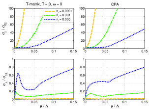
Figure 20: [color online] DC conductivities in the bilayer as a function of the chemical potential (in units of the cutoff) at zero temperature. Left: t-matrix; Right: CPA. Top: in plane; Bottom: c-axis.

The results for the DC conductivities at $T=0$ in the t-matrix and CPA approximations for different values of the chemical potential are shown in Figs. 20 and 21. The only difference between these figures are in the scales of the axes. It looks as if the minimum value for $\sigma_{\parallel}$ per plane in the bilayer is approximately $2\sigma_{\parallel 0}=4e^{2}/(\pi h)$, which is identical to the result one obtains using the same methods in single layer graphene.Peres et al. (2006) We discuss the minimum conductivity later in this section.

The low-energy feature in the t-matrix curves comes about at the energy scale at which the two planes start to decouple. The scale at which this takes place ($\Sigma_{\text{A}}\approx t_{\perp}$) is easily found numerically with the results shown in Table 2. The local maximum in the conductivities is readily identified with this energy scale.

$n_{\rm i}$	0.01	0.005	0.001	0.0001
$\omega/\Lambda$	$1.4\times 10^{-2}$	$6.5\times 10^{-3}$	$1.1\times 10^{-3}$	$8.4\times 10^{-5}$

Table 2: Energy scale $\omega$ at which the planes start to decouple within the t-matrix approximation [this happens when $\Sigma_{\text{A}}(\omega)\approx t_{\perp}$].

In the CPA this scale is suppressed and the curves show no peak. Quite generally it is seen that the CPA curves are smoother than the ones for the t-matrix.

Another interesting feature of $\sigma_{\perp}$ is that it is increased by disorder. This is due to the fact that disorder enhance the DOS on sublattice A where all the contribution to $\sigma_{\perp}$ is coming from. At the lowest values of the chemical potential the perpendicular conductivity still goes to zero however.

VIII.2 Minimal DC conductivity

By studying the curves more closely, it looks as if the CPA curves actually gives a value that is smaller than 2 in the limit $\omega\rightarrow 0$. In fact, we find that the minimum in the in-plane DC conductivity is again (as in the single layer case of massless Dirac fermions Peres et al. (2006)) universal in the sense of being independent of the particular impurity concentration. In the bilayer the minimum value per plane obtained from the CPA is

$$\sigma_{\parallel\text{min,CPA}}=\frac{3}{\pi}\frac{e^{2}}{h}.$$ (53)

This value is obtained by using the form of the self-energies in the low frequency limit that are given in Eq. (29). Explicitly one finds for the propagators via Eq. (21):

$${\rm g}_{\text{AA}}^{\text{D}}(\omega\rightarrow 0,{\bf k}) \sim \frac{\Sigma_{\text{B}}}{\xi\Lambda^{2}+k^{2}},$$ (54a)

$${\rm g}_{\text{BB}}^{\text{D}}(\omega\rightarrow 0,{\bf k}) \sim \frac{\Sigma_{\text{A}}}{\xi\Lambda^{2}+k^{2}},$$ (54b)

$${\rm g}_{\text{AB}}^{\text{ND}}(\omega\rightarrow 0,{\bf k}) \sim 0.$$ (54c)

Using these asymptotic forms in Eq. (47) and Eq. (48) the contribution from the latter equation drops out. The value in Eq. (53) is obtained from the first term after employing the relation: $\operatorname{Im}[\Sigma_{\text{A}}]\operatorname{Im}[\Sigma_{\text{B}}]\sim(\sqrt{3}/2)^{2}|\Sigma_{\text{A}}\Sigma_{\text{B}}|\sim 3\xi\Lambda^{2}/4$.

We note that our value for the minimal conductivity is different from the values obtained in works by other groups. In particular both Koshino and Ando (using a 2-band model in conjunction with a second-order self-consistent Boltzmann approximation) and Snyman and Beenakker (using the conductance formula for coherent transport) both finds the value $4e^{2}/(\pi h)$ per plane.Koshino and Ando (2006); Snyman and Beenakker (2007) (The minimal conductivity problem in bilayer graphene has also been discussed in Ref. [Katsnelson, 2006a; Cserti, 2007]). We can reproduce their result in our formalism by considering the case that the impurities only affect the B sublattice, as discussed in Sec. V.2 (or the case of Born scattering discussed in Sec. V.3). In particular, taking $\Sigma_{\text{A}}=0$ and $\Sigma_{\text{B}}(\omega=0)=-i\Gamma$ [from Eq. (31)] one finds

$${\rm g}_{\text{AA}}^{\text{D}}(\omega=0,{\bf k}) = \frac{-i\Gamma k^{2}}{(t_{\perp}\Gamma)^{2}+k^{4}},$$ (55a)

$${\rm g}_{\text{BB}}^{\text{D}}(\omega=0,{\bf k}) = \frac{-i\Gamma t_{\perp}^{2}}{(t_{\perp}\Gamma)^{2}+k^{4}},$$ (55b)

$${\rm g}_{\text{AB}}^{\text{ND}}(\omega=0,{\bf k}) = \frac{i\Gamma t_{\perp}k}{(t_{\perp}\Gamma)^{2}+k^{4}}.$$ (55c)

Using these expressions in Eq. (47) and Eq. (48), $\Xi_{x1,x1}$ and $\Xi_{x1,x2}$ are found to contribute equally to the conductivity with the total value being $4e^{2}/(\pi h)$. This result shows that the minimal conductivity is not really “universal” in the graphene bilayer since it actually depends on how the impurities are distributed among the inequivalent sites of the problem. Furthermore, the ballistic results corresponds to the case where the disorder is only affecting the B sublattice. Nevertheless, the general conclusion is that there is a non-zero minimum in the in-plane conductivity of the order of $e^{2}/h$. Further evidence for this conclusion is hinted by the related issue of how other hopping terms, such as $\gamma_{3}$ and $\gamma_{4}$, affect the value of the minimal conductivity. The case of trigonal warping (i.e. $\gamma_{3}\neq 0$) have been discussed in detail by Cserti and collaborators,Cserti et al. (2007) and they find that the minimal value of the conductivity per plane is $(12/\pi)(e^{2}/h)$ in this case (See App. A for an alternative derivation of this result). The introduction of $\gamma_{4}$ (or $\Delta$, or a next-nearest neighbor hopping within the planes) – which breaks the symmetry in energy between the central Dirac point and the three elliptical cones away from ${\bf k}=0$ will likely further influence the minimal value.

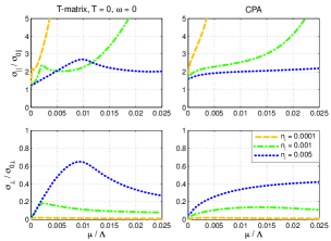
Figure 21: [color online] DC conductivities in the bilayer as a function of the chemical potential (in units of the cutoff) at zero temperature. Left: t-matrix; Right: CPA. Top: in plane; Bottom: c-axis.

VIII.3 Frequency dependence

The frequency dependence of the conductivities are pictured in Fig. 22-25. The figures reveals some interesting features of the band structure and the semimetallic behavior. For the case of a finite chemical potential the temperature does not make a big difference since it (at $300\,\text{K}$) is still much smaller than the Fermi energy, this is manifested in the small difference between Fig. 24 and Fig. 25. Near zero chemical potential the effect of the temperature is more dramatic. The temperature increase the number of carriers and is responsible for the Drude-like peaks that appear in the plots for low impurity concentrations. A well-known feature of semimetals is that the temperature is an important factor in determining the number of carriers in the system. The peak at $\omega\sim t_{\perp}=.05\Lambda$ is due to the onset of interband transitions. The frequency-dependence of the absorption of electromagnetic radiation has also been studied by Abergel and Falko with similar results,Abergel and Fal’ko (2007) they also study transitions between Landau levels in a magnetic field.

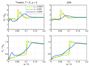
Figure 22: [color online] Conductivity as a function of frequency (in units of the cut-off) for the bilayer at the Dirac point $\mu=0$ for $T=0$. Left: t-matrix; Right: CPA. Top: in plane; Bottom: c-axis.

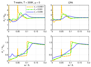
Figure 23: [color online] Conductivity as a function of frequency (in units of the cut-off) for the bilayer at finite temperature $T=300K$ near the Dirac point $\mu=0$. Left: t-matrix; Right: CPA. Top: in plane; Bottom: c-axis.

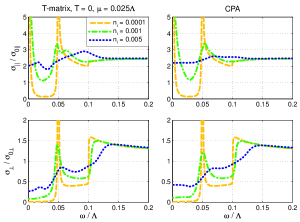
Figure 24: [color online] Conductivity as a function of frequency (in units of the cut-off) for the bilayer at finite chemical potential $\mu=0.025\Lambda$ at $T=0$. Left: t-matrix; Right: CPA. Top: in plane; Bottom: c-axis.

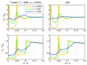
Figure 25: [color online] Conductivity as a function of frequency (in units of the cut-off) for the bilayer at finite temperature $T=300K$ at finite chemical potential $\mu=0.025\Lambda$. Left: t-matrix; Right: CPA. Top: in plane; Bottom: c-axis.

VIII.4 Temperature dependence

The temperature dependence of the DC conductivity can be found in Fig. 26 and Fig. 27. For the case of a finite chemical potential the in-plane conductivity curves are flat and proportional to $1/n_{i}$, as is expected in a normal Fermi liquid metal.Mahan (2000) The contribution to the scattering from impurities is very weakly temperature dependent. Nevertheless, there is a small temperature dependence for the lowest impurity concentration which is due to the fact that $T/E_{\text{F}}$ is still not negligible. Near the Dirac point the characteristics of a semimetal appear again as the conductivities become temperature dependent. Note however that we are not considering scattering by phonons which is important at finite temperatures.

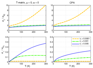
Figure 26: [color online] Temperature dependence of the DC conductivities in the bilayer at the Dirac point $\mu=0$. Left: t-matrix; Right: CPA. Top: in plane; Bottom: c-axis.

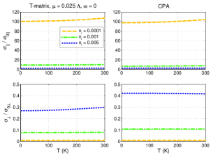
Figure 27: [color online] Temperature dependence of the DC conductivities in the bilayer at finite chemical potential $\mu=0.025\Lambda$.

IX Results for the conductivities in multilayer graphene

Using the same procedure as for the bilayer in the previous section we have calculated the kernels for arbitrary values of the self-energies. Details of this rather lengthy calculation are provided in App. C. In this section we present results for the conductivities using the kernels obtained with t-matrix and CPA self-energies discussed in Sec. VI.

The DC conductivities in the multilayer as a function of the chemical potential $\mu$ are pictured in Figs. 28-29, the only difference between the figures are in the scales of the axes. The property of disorder-enhanced transport in the perpendicular direction seems to survive in this model for the multilayer, but only for very low values of the chemical potential. For larger values of the chemical potential the influence of disorder becomes more conventional. In this case, because of the finite Fermi surface, the transport properties are more like in a normal metal.

IX.1 Perpendicular transport near the Dirac point

Generalizing Section V.3 to the multilayer we find again that $\Sigma_{\text{A}}\sim 0$ and $\Sigma_{\text{B}}\sim-i\Gamma_{\text{B}}$ is purely imaginary in the Born limit at the Dirac point. Nevertheless, as we shall see it is necessary for the computation of $\sigma_{\perp}$ that $\Sigma_{\text{A}}$ remain finite. Therefore we take $\Sigma_{\text{A}}\sim-i\Gamma_{\text{A}}$ and assume that $\Gamma_{\text{A}}\ll\Gamma_{\text{B}}$. We note that this is also consistent with a self-consistent version of the Born approximation for weak potentials. Thus, for $\omega\rightarrow 0$ we have

$$\operatorname{Im}[{\rm g}_{\text{AA}}^{\text{D}}] \sim \frac{-\Gamma_{\text{B}}(k^{2}+\Gamma_{\text{A}}\Gamma_{\text{B}})}{[2t_{\perp}\Gamma_{\text{B}}\cos(k_{\perp})]^{2}+(k^{2}+\Gamma_{\text{A}}\Gamma_{\text{B}})^{2}},$$ (56a)

$$\operatorname{Im}[{\rm g}_{\text{AA}}^{\text{ND}}] \sim 0.$$ (56b)

Inserting these expressions into Eq. (52) it is possible to perform the integrals exactly with the result

$$\Xi_{\perp,\text{multi}}\sim\frac{1}{d}\Bigl{(}\frac{4dt_{\perp}}{3at}\Bigr{)}^{2}\\ \times\Bigl{(}\frac{\Gamma_{\text{B}}}{8t_{\perp}}\Bigr{)}\log\Bigl{[}\frac{\sqrt{1+(\Gamma_{\text{A}}/2t_{\perp})^{2}}+1)}{\sqrt{1+(\Gamma_{\text{A}}/2t_{\perp})^{2}}-1)}\Bigr{]}.$$ (57)

Thus there is a logarithmic singularity in the limit $\Gamma_{\text{A}}\rightarrow 0$ as mentioned above. Intuitively this singularity comes from “clean” chains of atoms along the A sublattice where transport is unhindered once some weight has been pushed onto the A sublattice by the impurities on the B sublattice. It is plausible that $\Xi_{\perp,\text{multi}}$ increases with increasing disorder. It is so because the first factor grows linearly whereas the second factor decays only logarithmically with the $\Gamma$ in question.

For the case of vacancies in the CPA a result analogous to the one in Eq. (29) can be obtained. In fact the result is the same up to a factor: $\Sigma_{\text{A}}\rightarrow 2^{1/3}\Sigma_{\text{A}}$ and $\Sigma_{\text{B}}\rightarrow 2^{-1/3}\Sigma_{\text{B}}$. Therefore the asymptotic expressions in Eq. (54) are valid also in the multilayer. In addition one finds that ${\rm g}_{\text{AA}}^{\text{ND}}(\omega\rightarrow 0,{\bf k})\sim 0$. Thus, asymptotically one finds that $\Xi_{\perp,\text{multi}}\sim\omega^{2/3}$, which leads to a temperature dependence of $\sigma_{\perp}$ at the Dirac point that is of the form $T^{2/3}$. We also note that $\sigma_{\parallel,\text{min}}$ is independent of $t_{\perp}$ in the bilayer, thus we conclude that it takes on the same value in both the bilayer and the multilayer. Using the fact that $\Xi_{\parallel,\text{multi}}\sim$ constant at the Dirac point we find that $\sigma_{\parallel}/\sigma_{\perp}$ diverges as $T^{-2/3}$ as $T\rightarrow 0$ as reported previously.Nilsson et al. (2006a)

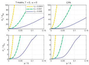
Figure 28: [color online] DC conductivities in the multilayer as a function of the chemical potential (in units of the cutoff) at T=0. Left: t-matrix; Right: CPA. Top: in plane; Bottom: c-axis.

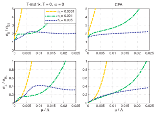
Figure 29: [color online] DC conductivities in the multilayer as a function of the chemical potential (in units of the cutoff) at T=0. Left: t-matrix; Right: CPA. Top: in plane; Bottom: c-axis.

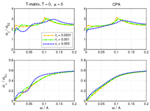
Figure 30: [color online] Conductivity as a function of frequency (in units of the cutoff) at the Dirac point $\mu=0$ for $T=0$ in the multilayer. Left: t-matrix; Right: CPA. Top: in plane; Bottom: c-axis.

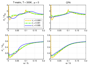
Figure 31: [color online] Conductivity as a function of frequency (in units of the cutoff) at finite temperature $T=300K$ near the Dirac point $\mu=0$ in the multilayer. Left: t-matrix; Right: CPA. Top: in plane; Bottom: c-axis.

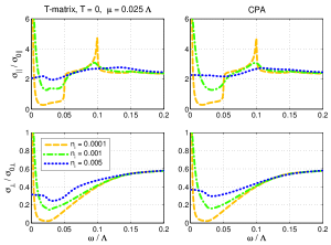
Figure 32: [color online] Conductivity as a function of frequency (in units of the cutoff) at finite chemical potential $\mu=0.025\Lambda$ at $T=0$ in the multilayer. Left: t-matrix; Right: CPA. Top: in plane; Bottom: c-axis.

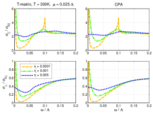
Figure 33: [color online] Conductivity as a function of frequency (in units of the cutoff) at finite temperature $T=300K$ at finite chemical potential $\mu=0.025\Lambda$ in the multilayer. Left: t-matrix; Right: CPA. Top: in plane; Bottom: c-axis.

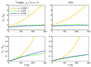
Figure 34: [color online] Temperature dependence of the DC conductivities at the Dirac point $\mu=0$ in the multilayer. Left: t-matrix; Right: CPA. Top: in plane; Bottom: c-axis.

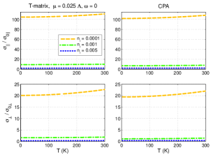
Figure 35: [color online] Temperature dependence of the DC conductivities at finite chemical potential $\mu=0.025\Lambda$ in the multilayer. Left: t-matrix; Right: CPA. Top: in plane; Bottom: c-axis.

IX.2 Frequency and temperature dependence

The frequency dependence of the conductivities in the multilayer is shown in Figs. 30-33 for two different temperatures and both at the Dirac point and for a finite chemical potential. For the cleaner systems a Drude-like peak appears at finite temperatures for both in-plane and perpendicular transport at the Dirac point. For a finite chemical potential – because the system is metallic in both directions – the system has a Drude peak in the conductivity also at zero temperature. Moreover, it can be seen how the suppression of the conductivity in the frequency range before interband contributions sets in (i.e. at $\omega=2\mu$) is affected by both disorder and temperature.

We note that our curves for the frequency-dependent in-plane conductivity is very similar to the recent results of Ref. Kuzmenko et al., , which include both measurements and calculations based on the full SWM model.

Our results for the temperature dependence of the conductivities in the multilayer are shown in Figs. 34-35. At the Dirac point, the in-plane conductivity goes to a finite constant while the perpendicular conductivity goes to zero as $T\rightarrow 0$. The disorder-enhanced transport at low temperatures can also be seen in the figure. For a finite chemical potential, the system behaves like a metal with only a weak temperature dependence of the conductivities.

X Impurities in the biased graphene bilayer

In the following sections we study the problem of impurities and mid-gap states in a biased graphene bilayer. We show that the properties of the bound states, such as localization lengths and binding energies, can be controlled externally by an electric field effect. Moreover, the band gap is renormalized and impurity bands are created at finite impurity concentrations. Using the CPA we calculate the electronic density of states and its dependence on the applied bias voltage. Many of the results we present here were previously reported in a brief form in Ref. [Nilsson and Castro Neto, 2007]. A recent detailed study of the impurity states in the unitary limit in both biased and unbiased bilayer graphene can be found in Ref. [Dahal et al., a].

X.1 Band model

In this section, we review the properties of the minimal model introduced in Eq. (10). Throughout this section we use units such that $v_{\rm F}=\hbar=1$ unless otherwise specified. For numerical estimates we use $t_{\perp}=.35\,\text{eV}$ and insert the appropriate factors of $v_{\rm F}=3ta/2$ with $t=3\,\text{eV}$ and $a=1.42\,\text{\AA}$. From Eq. (10) one finds two pairs of electron-hole symmetric eigenvalues:

$$E_{\pm,s}=\\ \pm\sqrt{k^{2}+\frac{V^{2}}{4}+\frac{t_{\perp}^{2}}{2}+s\frac{1}{2}\sqrt{4(V^{2}+t_{\perp}^{2})k^{2}+t_{\perp}^{4}}},$$ (58)

where $s=\pm$. The lowest energy bands (with respect to the “Dirac point” at zero energy) representing the valence and conduction bands are the $E_{\pm,-}$ bands. The smallest gap takes place at a finite wave vector given by

$$k_{\text{g}}=\frac{V}{2}\sqrt{\frac{V^{2}+2t_{\perp}^{2}}{V^{2}+t_{\perp}^{2}}},$$ (59)

so that the size of the band gap becomes

$$E_{\text{g}}=\frac{Vt_{\perp}}{\sqrt{V^{2}+t_{\perp}^{2}}}.$$ (60)

At $k=0$ the distance between the valence and the conduction band is given by the applied voltage difference $V$. Note that V should in reality be taken to be not the bare applied voltage difference but instead the self-consistently determined value $V_{\text{MF}}$ as discussed in Refs. [McCann, 2006; Min et al., 2007; Nilsson et al., 2007; Castro et al., 2007a]. Near $k_{\text{g}}$ the energy of the quasi-particles in the conduction band can be expanded as

$$E_{+,-}\approx\frac{Vt_{\perp}}{2\sqrt{V^{2}+t_{\perp}^{2}}}+\frac{V(V^{2}+2t_{\perp}^{2})}{t_{\perp}(V^{2}+t_{\perp}^{2})^{3/2}}(k-k_{\text{g}})^{2}\\ \equiv\frac{E_{\text{g}}}{2}+\frac{(k-k_{\text{g}})^{2}}{2m^{*}},$$ (61)

and as long as this approximation is valid the density of states per unit area is

$$N(\omega)=\frac{k_{0}}{\pi}\sqrt{\frac{2m^{*}}{|\omega|-E_{\text{g}}/2}},$$ (62)

for $|\omega|\geq E_{\text{g}}/2$. This includes both the valley and the spin degeneracy. Notice that the divergence of the density of states (DOS) at the band edge is similar to what one would get in a truly 1D system. The fact that a large DOS is accumulated near the band edge has important consequences for the properties of the bound states as we shall see in the following.

X.2 Bare Green’s function

An explicit expression for the bare Green’s function, which is given by ${\rm G}^{0}=\bigl{[}\omega-\mathcal{H}_{BB}\bigr{]}^{-1}$, is:

$${\rm G}^{0}=\frac{1}{D}\left(\begin{array}[]{ll}(\omega-V/2)\bigl{[}(\omega+V/2)^{2}-k^{2}\bigr{]}&\bigl{[}(\omega+V/2)^{2}-k^{2}\bigr{]}ke^{i\phi}\\ \bigl{[}(\omega+V/2)^{2}-k^{2}\bigr{]}ke^{-i\phi}&(\omega-V/2)\bigl{[}(\omega+V/2)^{2}-k^{2}\bigr{]}-(\omega+V/2)t_{\perp}^{2}\\ t_{\perp}(\omega^{2}-V^{2}/4)&t_{\perp}(\omega+V/2)ke^{i\phi}\\ t_{\perp}(\omega-V/2)ke^{i\phi}&t_{\perp}k^{2}e^{2i\phi}\end{array}\right.\\ \left.\begin{array}[]{ll}t_{\perp}\left(\omega^{2}-V^{2}/4\right)&t_{\perp}(\omega-V/2)ke^{-i\phi}\\ t_{\perp}(\omega+V/2)ke^{-i\phi}&t_{\perp}k^{2}e^{-2i\phi}\\ (\omega+V/2)\bigl{[}(\omega-V/2)^{2}-k^{2}\bigr{]}&\bigl{[}(\omega-V/2)^{2}-k^{2}\bigr{]}ke^{-i\phi}\\ \bigl{[}(\omega-V/2)^{2}-k^{2}\bigr{]}ke^{i\phi}&(\omega+V/2)\bigl{[}(\omega-V/2)^{2}-k^{2}\bigr{]}-(\omega-V/2)t_{\perp}^{2}\end{array}\right),$$ (63)

where

$$D = \bigl{[}k^{2}-V^{2}/4-\omega^{2}\bigr{]}^{2}+M^{4},$$ (64)

$$M^{4} = \frac{V^{2}t_{\perp}^{2}}{4}-\omega^{2}(V^{2}+t_{\perp}^{2}).$$ (65)

So that, for example, the important diagonal components are given by

$${\rm G}^{0}_{\text{A}1\text{A}1} = \frac{(\omega-V/2)\bigl{[}(\omega+V/2)^{2}-k^{2}\bigr{]}}{D},$$ (66a)

$${\rm G}^{0}_{\text{B}1\text{B}1} = {\rm G}^{0}_{\text{A}1\text{A}1}-\frac{(\omega+V/2)t_{\perp}^{2}}{D}.$$ (66b)

The corresponding components for plane 2 are obtained by the substitution $V\rightarrow-V$. Note that $M>0$ inside of the gap.

XI Bound states for Dirac delta potentials

Bound states must be located inside of the gap so that their energies fulfill $|\epsilon|<E_{\text{g}}/2$, otherwise the asymptotic states at infinity are not exponentially localized. If we decode a number (say $N_{i}$) of local impurities in a matrix of the form

$$\hat{V}=\text{Diag}[U_{1},\,U_{2}\,,\ldots,\,U_{N_{i}}],$$ (67)

where we let $U_{i}$ denote the strength of the impurity potential that is located at site ${\bf x}_{i}$. The total Green’s function is then given by

$${\rm G}={\rm G}^{0}+{\rm G}^{0}\hat{V}{\rm G}={\rm G}^{0}+{\rm G}^{0}\hat{V}{\rm G}^{0}+{\rm G}^{0}\hat{V}{\rm G}^{0}\hat{V}{\rm G}^{0}+\ldots\\ ={\rm G}^{0}+{\rm G}^{0}\bigl{[}\hat{V}+\hat{V}{\rm G}^{0}\hat{V}+\hat{V}{\rm G}^{0}\hat{V}{\rm G}^{0}\hat{V}+\ldots\bigr{]}{\rm G}^{0}\\ \equiv{\rm G}^{0}+{\rm G}^{0}T{\rm G}^{0}.$$ (68)

Here $T$ is the t-matrix of the system (see e.g. Ref. [Jones and March, 1985]). The interpretation of this expression is most transparent in the real space picture, where it includes the repeated scattering off of all of the impurities in every possible way. Another way of expressing $T$ is (decomposing $\hat{V}$ as $\hat{V}=\sqrt{\hat{V}}\sqrt{\hat{V}}$):

$$T=\sqrt{\hat{V}}(1+\sqrt{\hat{V}}{\rm G}^{0}\sqrt{\hat{V}}+(\sqrt{\hat{V}}{\rm G}^{0}\sqrt{\hat{V}})^{2}+\ldots)\sqrt{\hat{V}}\\ =\sqrt{\hat{V}}\frac{1}{1-\sqrt{\hat{V}}{\rm G}^{0}\sqrt{\hat{V}}}\sqrt{\hat{V}}.$$ (69)

Bound states generated by the impurities can readily be identified by the possibly new poles in the full propagator of the system. Therefore an equation that can be solved to find the energies of the bound states of the system is given by

$$\text{Det}\Bigl{[}\delta_{i,j}-\sqrt{U_{i}}{\rm G}^{0}_{ij}(\epsilon)\sqrt{U_{j}}\,\Bigr{]}=0.$$ (70)

Here ${\rm G}^{0}_{ij}(\epsilon)$ denotes the (real space) propagator from site $j$ to site $i$. In principle one can put in an arbitrary number of impurities in this expression. However, if two impurities are located too close to each other the continuum approximation to the propagators is not expected to be accurate and one must instead work with the full tight-binding description (see Ref. [Wehling et al., 2007] for an illustration of this approach in monolayer graphene). If we specialize to one local impurity affecting only one site the calculations simplify considerably. The Fourier transform of the local potential is $U/N$ (where $N$ is the number of unit cells in the system) so that we can write

$$T=\frac{1}{N}\frac{U}{1-U\overline{{\rm G}}^{0}}.$$ (71)

As mentioned previously, to locate the bound states we must find possible new poles due to the potential. Explicitly we need $U\overline{{\rm G}}^{0}(\epsilon)=1$. Like in Section V, $\overline{{\rm G}}^{0}$ is the local propagator at the impurity site that is given by the expression in Eq. (25) with ${{\rm G}}^{0}$ taken from Eq. (63). Using Eq. (66) we can perform the integrals exactly in the continuum approximation with the result

$$\overline{{\rm G}}_{\text{A}1}^{0}=\frac{V/2-\omega}{2\Lambda^{2}}\Bigl{\{}\log\Bigl{(}\frac{\Lambda^{4}}{M^{4}+(V^{2}/4+\omega^{2})^{2}}\Bigr{)}\\ -\frac{2\omega V}{M^{2}}\Bigl{[}\tan^{-1}\Bigl{(}\frac{V^{2}/4+\omega^{2}}{M^{2}}\Bigr{)}+\tan^{-1}\Bigl{(}\frac{\Lambda^{2}}{M^{2}}\Bigr{)}\Bigr{]}\Bigr{\}},$$ (72a)

$$\overline{{\rm G}}_{\text{B}1}^{0}=\overline{{\rm G}}_{\text{A}1}^{0}-\frac{({V/2}+\omega)t_{\perp}^{2}}{M^{2}\Lambda^{2}}\Bigl{[}\tan^{-1}\Bigl{(}\frac{\Lambda^{2}}{M^{2}}\Bigr{)}\\ +\tan^{-1}\Bigl{(}\frac{V^{2}/4+\omega^{2}}{M^{2}}\Bigr{)}\Bigr{]},$$ (72b)

where $M^{2}=\sqrt{V^{2}t_{\perp}^{2}/4-\omega^{2}(V^{2}+t_{\perp}^{2})}$, and $\Lambda$ ($\approx 7$ eV) is the high energy cutoff. The corresponding expressions in plane 2 are obtained by the substitution $V\rightarrow-V$. The typical behavior of $\overline{{\rm G}}^{0}(\omega)$ as a function of the frequency $\omega$ is shown in Fig. 36.

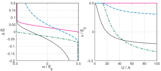
Figure 36: [color online] Left: typical behavior of the $\overline{{\rm G}}^{0}$’s: $\overline{{\rm G}}_{\text{B}1}^{0}(\omega)$ (dotted), $\overline{{\rm G}}_{\text{B}2}^{0}(\omega)$ (dashed), $\overline{{\rm G}}_{\text{A}1}^{0}(\omega)$ (solid), $\overline{{\rm G}}_{\text{A}2}^{0}(\omega)$ (dash-dotted). Here $V=50\,\text{meV}$. The divergences close to the band edges are clearly visible. Right: bound state energies $\epsilon$ for a local potential of strength $-U$, the labeling of the sublattices is the same as to the left.

From this we conclude that a Dirac delta potential always generates a bound state (no matter how weak the potential is) since $\overline{{\rm G}}^{0}$ diverges as the band edge is approached (where $M\rightarrow 0$). The dependence on the cutoff (except for the overall scale) is rather weak so that the linear in-plane approximation to the spectrum should be a good approximation as in the case of graphene.Wehling et al. (2007) For a given strength of the potential $U$, there are four different bound state energies depending on which lattice site it is sitting on. In Fig. 36 we show the energies of these bound states for strong impurities. Even at these scales the bound state coming from $\overline{{\rm G}}_{\text{A}1}^{0}$ is so weakly bound that it is barely visible in the figure. In Fig. 37 we show the binding energy as a function of $U$ and $V$ for the deepest bound state (coming from $\overline{{\rm G}}_{\text{B}1}^{0}$). In the limit of $U\rightarrow\infty$ the electron-hole symmetry of the bound state energies is restored.

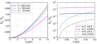
Figure 37: [color online] Left: Bound state binding energies $E_{\text{b}}$ (in units of the gap $E_{\text{g}}$) for a Dirac delta potential of strength $-U$ for different bias $V$. Right: Binding energies of a potential well of range $R=10\,a$ and strength $\gamma=\gamma_{1}=\gamma_{2}$ (see the text in Sec. XIV) for different angular momentum $m$ channels and external bias potential $V$.

For illustrative purposes we consider only attractive potentials in this work, analogous results hold for repulsive potentials because of the electron-hole symmetry of the model that we are using. For smaller values of the potential ($|U|\ll\Lambda$) the binding energy measured from the band edge $E_{\text{b}}=E_{\text{g}}/2-\epsilon$ grows as $U^{2}$ and the states are weakly bound. For example, for $V=40\,\text{meV}$ and $U\lesssim 1\text{eV}$ one finds $E_{\text{b}}\lesssim 4\times 10^{-4}E_{\text{g}}$.

XI.1 Angular momentum states

For any potential with cylindrical symmetry it is useful to classify the eigenstates according to their angular momentum $m$. In the presence of the “trigonal distortion” parametrized by $\gamma_{3}$ the calculations become more involved because of the broken cylindrical symmetry. We discuss this issue briefly in Sec. XVI. The real space continuum version of the Hamiltonian matrix in Eq. (10) that includes a potential, which in general is allowed to take on different values in the two planes, is

$$\mathcal{H}_{0}=\begin{pmatrix}V/2+g_{1}(r)-i\sigma^{*}\cdot\partial&t_{\perp}(1+\sigma_{z})/2\\ t_{\perp}(1+\sigma_{z})/2&-V/2+g_{2}(r)-i\sigma\cdot\partial\end{pmatrix}.$$ (73)

Here $\sigma_{i}$ ($i=x,y,z$) are the usual Pauli matrices. For example, a symmetric Coulomb problem could then be approximated by taking $g_{1}(r)=g_{2}(r)=g/r$. Going to cylindrical coordinates the derivatives transforms according to

$$\partial_{x}\pm i\partial_{y}=e^{\pm i\varphi}(\partial_{r}\pm\frac{i}{r}\partial_{\varphi}),$$ (74)

where we use the coordinate convention $x\pm iy=re^{\pm i\varphi}$. For the Hamiltonian in Eq. (73) one can now – in analogy with the usual Dirac equation DiVincenzo and Mele (1984) – construct an angular momentum operator that commutes with the Hamiltonian. The angular ($\varphi$) dependence of the angular momentum $m$ eigenstates are those of the vector:

$$u_{\alpha,m}(\varphi)=e^{im\varphi}\begin{pmatrix}1\\ e^{-i\varphi}e^{-i\alpha\pi/2}\\ 1\\ e^{i\varphi}e^{i\alpha\pi/2}\end{pmatrix},$$ (75)

where parameter $\alpha$ is introduced for later convenience, it is used later to obtain more compact expressions. It is convenient to define the following “star” product of two vectors that results in another vector with components given by

$$[\,a\star b\,]_{\alpha j}=a_{\alpha j}\,b_{\alpha j}.$$ (76)

By writing $\Psi=u_{0,m}\star\psi(r)/\sqrt{r}$ the eigenvalue problem $\mathcal{H}_{0}\Psi=E\Psi$ is transformed into a set of coupled ordinary linear differential equations for the radial wave-function $\psi(r)$:

$$\begin{pmatrix}g_{1}(r)+V/2&-i\partial_{r}+i\,j/r&t_{\perp}&0\\ -i\partial_{r}-i\,j/r&g_{1}(r)+V/2&0&0\\ t_{\perp}&0&g_{2}(r)-V/2&-i\partial_{r}-i\,(j+1)/r\\ 0&0&-i\partial_{r}+i\,(j+1)/r&g_{2}(r)-V/2\end{pmatrix}\psi(r)=E\psi(r).$$ (77)

Here we have introduced $j=m-1/2$ to render the equations more symmetric. If the potential generates bound states inside of the gap these states decay exponentially $\sim r^{\gamma}e^{-\kappa r}$ as $r\rightarrow\infty$. Assuming that the potential decays fast enough the asymptotic behavior of Eq. (77) imply that the allowed values for $\kappa$ are $\kappa_{\pm}$ satisfying

$$\kappa_{\pm} = \sqrt{-(\epsilon^{2}+V^{2}/4)\pm iM^{2}},$$ (78a)

$$|\kappa|^{4} = (V^{2}/4-\epsilon^{2})(V^{2}/4-\epsilon^{2}+t_{\perp}^{2}),$$ (78b)

$$\kappa_{\pm} = |\kappa|\exp\Bigl{\{}\pm i\bigl{[}\frac{\pi}{2}-\frac{1}{2}\tan^{-1}\Bigl{(}\frac{M^{2}}{\epsilon^{2}+V^{2}/4}\Bigr{)}\bigr{]}\Bigr{\}}.$$ (78c)

So that, for weakly bound states we have

$$\kappa_{\pm}\approx\frac{M^{2}}{\sqrt{V^{2}+E_{\text{g}}^{2}}}\pm i\frac{1}{2}\sqrt{V^{2}+E_{\text{g}}^{2}},$$ (79)

leading to a localization length

$$l\sim\frac{2k_{\text{g}}}{Vt_{\perp}}\sqrt{\frac{E_{\text{g}}}{E_{\text{b}}}},$$ (80)

that diverges as the band edge is approached and decreases as the bias voltage increases.

XI.2 Free particle wave functions in the angular momentum basis

The free particle wave functions in the angular momentum basis can be conveniently expressed in terms of the following vectors:

$$v_{Z,m}(z)=\begin{pmatrix}Z_{m}(z)\\ Z_{m-1}(z)\\ Z_{m}(z)\\ Z_{m+1}(z)\end{pmatrix},$$ (81)

$$w(p)=\begin{pmatrix}\bigl{[}(\omega+{V/2})^{2}-p^{2}\bigr{]}(\omega-{V/2})\\ \bigl{[}(\omega+{V/2})^{2}-p^{2}\bigr{]}p\\ t_{\perp}(\omega^{2}-V^{2}/4)\\ t_{\perp}(\omega-{V/2})p\end{pmatrix}.$$ (82)

The last vector is useful as long as $\omega\neq{V/2}$ (cf. the discussion of the two eigenvectors in Ref. [Nilsson et al., 2007].) The denominator (actually a determinant) that determines the eigenstates is:

$$D(p,\omega)=\bigl{[}p^{2}-V^{2}/4-\omega^{2}\bigr{]}^{2}+V^{2}t_{\perp}^{2}/4-\omega^{2}(V^{2}+t_{\perp}^{2}).$$ (83)

Then, provided that $D(k,\omega)=0$, ($k>0$) which corresponds to propagating modes, the eigenfunctions are proportional to:

$$\Psi_{Z,m}(\omega,k,r)=u_{1,m}\star v_{Z,m}(kr)\star w(k),$$ (84)

where $Z_{m}(x)=J_{m}(x)$ or $Y_{m}(x)$ are Bessel functions and the star product is defined in Eq. (76). If on the other hand $D(i\kappa,\omega)=0$, ($\text{Re}[\kappa]>0$) the eigenfunctions are instead:

$$\Psi_{K,m}(\omega,\kappa,r) = u_{0,m}\star v_{K,m}(\kappa r)\star w(i\kappa),$$ (85)

$$\Psi_{I,m}(\omega,\kappa,r) = u_{0,m}\star v_{I,m}(\kappa r)\star w(-i\kappa),$$ (86)

with $I_{m}(x)$ and $K_{m}(x)$ being modified Bessel functions. That these vectors are indeed free-particle eigenstates can be verified straightforwardly by applying the Hamiltonian in Eq. (73) with $g_{1}=g_{2}=0$ to them.

XI.3 Local impurity wave functions

The general expression for the retarded Green’s function is

$${\rm G}_{\alpha j,\alpha^{\prime}j^{\prime}}({\bf x},{\bf x}^{\prime})=\sum_{n}\frac{\langle\alpha j,{\bf x}|n\rangle\langle n|\alpha^{\prime}j^{\prime},{\bf x}^{\prime}\rangle}{\omega+i\delta-E_{n}},$$ (87)

where the sum is over the eigenstates $|n\rangle$ (with eigenenergy $E_{n}$) of the system. Comparing the coefficient of the poles in this expression with those in Eq. (68) one can read of the wave functions of the bound states directly. The result is that the wave functions are Fourier transforms of the columns of the bare Green’s evaluated with the frequency set to be equal to the energy of the bound state.

XI.3.1 Impurity on an A1 site

When the impurity is on an A1 site the expression becomes [using Eq. (63)]

$$\begin{pmatrix}{\rm G}_{\text{A}1\text{A}1}\\ {\rm G}_{\text{B}1\text{A}1}\\ {\rm G}_{\text{A}2\text{A}1}\\ {\rm G}_{\text{B}2\text{A}1}\end{pmatrix}=\frac{1}{N}\sum_{{\bf k}}\frac{e^{i{\bf k}\cdot{\bf x}}}{D}\begin{pmatrix}(\omega-V/2)\bigl{[}(\omega+V/2)^{2}-k^{2}\bigr{]}\\ \bigl{[}(\omega+V/2)^{2}-k^{2}\bigr{]}ke^{\mp i\phi}\\ t_{\perp}(\omega^{2}-V^{2}/4)\\ t_{\perp}(\omega-V/2)ke^{\pm i\phi}.\end{pmatrix}.$$ (88)

Performing the angular average one ends up with Bessel functions:

$$\begin{pmatrix}{\rm G}_{\text{A}1\text{A}1}\\ {\rm G}_{\text{B}1\text{A}1}\\ {\rm G}_{\text{A}2\text{A}1}\\ {\rm G}_{\text{B}2\text{A}1}\end{pmatrix}=\int_{0}^{\Lambda}\frac{kdk}{\Lambda^{2}D}\begin{pmatrix}(\omega-V/2)\bigl{[}(\omega+V/2)^{2}-k^{2}\bigr{]}J_{0}(kr)\\ i\bigl{[}(\omega+V/2)^{2}-k^{2}\bigr{]}kJ_{1}(kr)e^{-i\varphi}\\ t_{\perp}(\omega^{2}-V^{2}/4)J_{0}(kr)\\ it_{\perp}(\omega-V/2)kJ_{1}(kr)e^{i\varphi}\end{pmatrix}.$$ (89)

There are really two such terms, one for each K-point, which corresponds to the different signs of the phases in Eq. (88). Note that this state has angular momentum $m=0$ in the language of the Section XI.1. The $k$-integral can be performed analytically (taking $\Lambda\rightarrow\infty$ in the integration limit). Using $\kappa_{\pm}$ defined in Eq. (78) we obtain

$${\rm G}_{\text{A}1\text{A}1} = \frac{V/2-\omega}{2}\sum_{\alpha=\pm}\Bigr{\{}1-i\alpha\frac{V\omega}{M^{2}}\Bigr{\}}K_{0}(\kappa_{\alpha}r),$$ (90a)

$${\rm G}_{\text{B}1\text{A}1} = \frac{-i}{2}\sum_{\alpha=\pm}\Bigr{\{}1-i\alpha\frac{V\omega}{M^{2}}\Bigr{\}}\bigl{[}\kappa_{\alpha}K_{1}(\kappa_{\alpha}r)\bigr{]}e^{-i\varphi},$$ (90b)

$${\rm G}_{\text{A}2\text{A}1} = \frac{-it_{\perp}(V^{2}/4-\omega^{2})}{2M^{2}}\sum_{\alpha=\pm}\bigl{[}\alpha K_{0}(\kappa_{\alpha}r)\bigr{]},$$ (90c)

$${\rm G}_{\text{B}2\text{A}1} = \frac{t_{\perp}(V/2-\omega)}{2M^{2}}\sum_{\alpha=\pm}\bigl{[}\alpha\kappa_{\alpha}K_{1}(\kappa_{\alpha}r)\bigr{]}e^{i\varphi}.$$ (90d)

These propagators can also be easily expressed in terms of the free-particle wave functions:

$${\rm G}_{\alpha j,\text{A}1}=\Bigr{[}\frac{\Psi_{K,0}(\epsilon,\kappa_{+},r)-\Psi_{K,0}(\epsilon,\kappa_{-},r)}{-i2M^{2}\Lambda^{2}}\Bigr{]}_{\alpha j}.$$ (91)

This property is not a coincidence since the particles are essentially free, except for the potential that acts on the single impurity site at the origin.

XI.3.2 Impurity on a B1 site

When there is an impurity on a B1 site one can perform the same calculation with the result that the wave function becomes

$${\rm G}_{\alpha j,\text{B}1}=\Bigl{[}\frac{\kappa_{+}\Psi_{K,1}(\epsilon,\kappa_{+},r)-\kappa_{-}\Psi_{K,1}(\epsilon,\kappa_{-},r)}{2M^{2}\Lambda^{2}({V/2}-\epsilon)}\Bigr{]}_{\alpha j}.$$ (92)

This state has angular momentum $m=1$ in the language of Sec. XI.1. A similar expression can be obtained when there is an impurity on an $\text{A}2$ ($\text{B}2$) site, where in this case the corresponding state has angular momentum $m=0$ ($m=-1$).

XI.4 Asymptotic behavior

The asymptotic behavior of the modified Bessel functions is $K_{n}(z)\sim\exp(-z)/\sqrt{z}$ as $z\rightarrow\infty$. Therefore the bound states are exponentially localized within a length scale given by [See Eq. (78)]

$$l=\bigl{\{}\operatorname{Re}(\kappa_{\pm})\bigr{\}}^{-1}\\ =\biggl{(}\sqrt[4]{(\epsilon^{2}+V^{2}/4)^{2}+M^{4}}\sin\Bigr{\{}\frac{1}{2}\tan^{-1}\Bigl{[}\frac{M^{2}}{(\epsilon^{2}+V^{2}/4)^{2}}\Bigr{]}\Bigl{\}}\biggr{)}^{-1}\\ \approx\frac{2k_{\text{g}}}{Vt_{\perp}}\sqrt{\frac{2}{1-2|\epsilon|/E_{\text{g}}}},$$ (93)

where the last line is applicable for weakly bound states close to the band edge. This is in agreement with the general results above in Eq. (80). At short distances one may use that $K_{n}(z)\sim 1/z^{n}$ for $n\geq 0$ and $K_{0}(z)\sim-\ln z$ to conclude that the wave functions are not normalizable in the continuum. In particular, for an impurity on the $\text{A}1$ ($\text{B}1$) site the wave function on the $\text{B}1$ ($\text{A}1$) site diverges as $1/r$. This divergence is however rather weak (i.e., logarithmic) and not real since in a proper treatment of the short-distance physics, the divergence is cutoff by the lattice spacing $a$ (this is equivalent to cutting of the $k$-integral in Eq. (89) at $k=\Lambda$ instead of taking $\Lambda\rightarrow\infty$).

XII Simple criterion

Using the asymptotic form of the wave functions one can approximate the wave function as:

$$\psi\sim\frac{A}{\sqrt{2r}}e^{-\kappa r},$$ (94)

in each plane. Normalization then requires that $A=\sqrt{\kappa^{\prime}/\pi}$, where $\kappa^{\prime}$ is the real part of $\kappa_{\pm}$. Thus one impurity is interacting with approximately

$$N_{l}=\langle\pi r^{2}\rangle/\frac{3\sqrt{3}a^{2}}{4}$$ (95)

atoms per plane. For an impurity density of $n_{i}$, the number of impurities interacting with a given impurity is given by

$$N_{i}=\frac{\pi\sqrt{3}}{2}\Bigl{(}\frac{t}{\kappa^{\prime}}\Bigr{)}^{2}n_{\rm i}.$$ (96)

A simple estimate of the critical density $n_{c}$ above which the interaction between different impurities are important is then given by $N_{i}\sim 1$. Writing $\epsilon=E_{\text{g}}/2-E_{\text{b}}$ one then finds the following criterion for overlap of impurity wave functions (assuming weakly binding impurities):

$$n_{\rm i}\gtrsim n_{c}=\frac{1}{2\pi\sqrt{3}}\Bigl{(}\frac{Vt_{\perp}}{k_{\text{g}}t}\Bigr{)}^{2}\frac{E_{\text{b}}}{E_{\text{g}}}\approx 2.5\times 10^{-3}\frac{E_{\text{b}}}{E_{\text{g}}},$$ (97)

indicating that the critical density increases with the applied gate voltage. The last step is valid for $V\ll t_{\perp}$. Taking $U\lesssim 1\,\text{eV}$ we found in Section XI that $E_{\text{b}}\lesssim 4\times 10^{-4}E_{\text{g}}$, leading to $n_{c}\sim 10^{-6}$. Hence, even tiny concentrations of impurities lead to wave function overlap. This result shows that even a small amount of impurities can have strong effects in the electronic properties of the BGB.

XIII Variational calculations

For general potentials it is not possible to solve for the bound states in closed form. Nevertheless, for estimates and to gain intuition about the problem it is fruitful to study the problem with variational techniques. In this section we consider two different variational approaches.

XIII.1 Variational calculation I

Using Eq. (77) one can show the existence of bound states variationally. For simplicity we consider only the case $m=0$ ($j=-1/2$) and a symmetric potential $g_{1}=g_{2}=g(r)$. We use the simple trial wave function $\psi_{2}=A\exp(-kr/2)$. The following integrals are useful in the process:

$$\int_{0}^{\infty}|\psi_{2}|^{2}dr = 1,$$ (98a)

$$\int_{a}^{\infty}\frac{|\psi_{2}|^{2}}{r}dr = kE_{1}(ka),$$ (98b)

$$\int_{0}^{\infty}\Theta(R-r)|\psi_{2}|^{2}dr = 1-\exp(-kR).$$ (98c)

Here $a$ is a cutoff on the order of the lattice spacing needed to regularize the integral. $E_{1}(x)=\int_{x}^{\infty}dr\exp(-r)/r$ is an exponential integral (see e.g. Ref. [Gradshteyn and Ryzhik, 2000]). The eigenvalues ($\epsilon_{k}$) of the kinetic term is given by the equation

$$0=\Bigl{\{}{\epsilon}^{2}+\frac{V^{2}}{4}-\frac{k^{2}}{4}\bigl{[}E_{1}(ka)^{2}-1\bigr{]}\Bigr{\}}^{2}+\frac{V^{2}t_{\perp}^{2}}{4}-{\epsilon}^{2}(V^{2}+t_{\perp}^{2}),$$ (99)

which is the same as the equation for the bare bands [cf. Eq. (64)] with the substitution $k^{2}\rightarrow k^{2}[E_{1}(ka)^{2}-1]/4$. Provided that $ka\lesssim 0.26$ ($k\lesssim 1.2\,\text{eV}$) the new “momentum” is real. For an attractive potential we may then construct a wave packet corresponding to the $E_{+,-}$ band leading to a positive contribution from the kinetic term.

We consider two types of potentials: one of the Coulomb type, $g_{C}=-\alpha/r$, characterized by the dimensionless strength $\alpha$; and a local potential, $g_{L}=-U\Theta(R-r)$, characterized by the strength $U$ and the range $R$. The total variational energies for the two types of potentials are:

$$E_{\text{var},C} = E_{+,-}\Bigl{(}\frac{k}{2}\sqrt{E_{1}(ka)^{2}-1}\Bigr{)}-\alpha kE_{1}(ka),$$ (100a)

$$E_{\text{var},L} = E_{+,-}\Bigl{(}\frac{k}{2}\sqrt{E_{1}(ka)^{2}-1}\Bigr{)}-U[1-e^{-kR}].$$ (100b)

Some typical results obtained from these expression are shown in Figs. 38 and 39. For a sufficiently strong potential it is favorable for the state to become very localized close to the impurity, and the assumed “bound state” is located inside of the continuum of the valence band. This is problematic as it leads to a breakdown of the picture of a bound state coming only from the states in the $E_{+,-}$ band. The state can no longer be considered a true bound state since it is allowed to hybridize with the states in the valence band and hence leak away into infinity. This state can therefore only be regarded as a resonance. Nevertheless, for weak Coulomb potentials there are indeed bound states inside of the gap, and for short-range potentials the variational treatment give results that are consistent with the more rigorous study coming up in Section XIV.

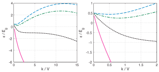
Figure 38: [color online] Variational energy for a Coulomb potential as a function of the variational parameter $k$ for $V=50\,\text{meV}$. From top to bottom: $\alpha=.033$, $.1$, $.33$, and $1$. Left: large view; Right: zoom in for small $k$.

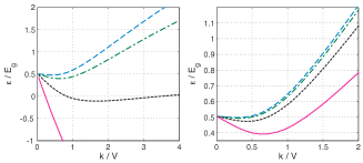
Figure 39: [color online] Variational energy for a short-range potential of range $R$ as a function of the variational parameter $k$ for $V=50\,\text{meV}$. From top to bottom: $U=.033$, $.1$, $.33$, and $1$ eV. Left: $R=10\,a$; Right: $R=1\,a$.

XIII.2 Variational calculation II

Another simple variational approach is to construct a wave packet with angular momentum $m$ and a momentum close to $k_{g}$ from the $E_{+-}$ band using the free particle solutions in Eq. (84) according to:

$$\Psi_{\text{var}}(\xi)=\int_{k_{g}-\xi}^{k_{g}+\xi}dp\,\Psi_{J,m}(E_{+-}(p),p,r)\,\sqrt{\frac{p}{4\pi\xi}},$$ (101)

where we assume that $\xi\ll k_{\text{g}}$. The factor $\sqrt{p/\xi}$ is included to generate a properly normalized variational state. Since this state is built up of eigenstates of the kinetic term the contribution from the kinetic energy to the variational energy becomes:

$$E_{\text{var,kin}}\approx\frac{1}{\xi}\int_{k_{g}-\xi}^{k_{g}+\xi}dp\frac{p^{2}}{2m^{*}}=\frac{\xi^{2}}{3m^{*}},$$ (102)

using Eq. (61). The leading contribution to the interaction energy for small $\xi$ becomes:

$$E_{\text{var,int}}=\int d^{2}{\bf x}\int_{k_{g}-\xi}^{k_{g}+\xi}dp\int_{k_{g}-\xi}^{k_{g}+\xi}dp^{\prime}\\ \times\frac{\sqrt{p\,p^{\prime}}}{{4\pi\xi}}\Psi^{{\dagger}}_{J,m}(E_{+-}(p),p,r)g(r)\Psi_{J,m}(E_{+-}(p^{\prime}),p^{\prime},r)\\ \approx 2\xi k_{\text{g}}\int drr\Psi^{{\dagger}}_{J,m}(E,k_{\text{g}},r)g(r)\Psi_{J,m}(E,k_{\text{g}},r)\Bigr{|}_{E=E_{+-}(k_{\text{g}})}\\ \equiv-2\xi k_{\text{g}}\frac{U}{\widetilde{R}^{2}}.$$ (103)

Therefore, the variational calculation shows that for any $m$, a weak attractive potential of strength $\propto U$ leads to a weakly bound state with binding energy $E_{\text{b}}\propto U^{2}$. This can be understood by noting that for each value of $m$, due to $k_{\text{g}}$ being nonzero, the problem maps into a 1D system with an effective local potential. It is well known (see e.g. Ref. [Landau and Lifshitz, 1977]) that in 1D a weak attractive potential ($\propto U$) always leads to a bound state with binding energy $E_{\text{b}}\propto U^{2}$. Thus the result is a direct consequence of the peculiar topology of the BGB band edge – see however Sec. XVI.

XIV Potential well

For the case of the simple local “potential well” defined by the potentials $g_{Lj}=-U_{j}\Theta(R-r)\equiv-\gamma_{j}\Theta(R-r)/R$ it is possible to make analytic progress with the continuum problem. In Sec. XI.2 we gave the explicit form of the eigenstates for a constant potential in the angular momentum basis. Bound states are possible when the two solutions for $r<R$ and the two solutions for $r>R$ are not linearly independent at $r=R$. This can be tested by evaluating the $4\times 4$ determinant of the matrix built up by the four eigenstate spinors. Given $U_{1}$, $U_{2}$ and $R$ the resulting determinant is a function of the energy $\omega$. Zeros of the determinant inside of the band gap corresponds to the bound states that we are searching for. Inside of the potential region the effective frequency and bias are given by:

$$\widetilde{\omega} = \omega+(U_{1}+U_{2})/2,$$ (104a)

$$\widetilde{V} = V+(U_{2}-U_{1}).$$ (104b)

The determinant is given by one of the following expressions:

$$D_{0}(\omega) = \text{Det}\bigl{[}\Psi_{K,m}(\omega,\kappa_{+},R),\,\Psi_{K,m}(\omega,\kappa_{-},R),\,\Psi_{I,m}(\widetilde{\omega},\widetilde{\kappa}_{+},R),\,\Psi_{I,m}(\widetilde{\omega},\widetilde{\kappa}_{-},R)\bigr{]},$$

$$D_{1}(\omega) = \text{Det}\bigl{[}\Psi_{K,m}(\omega,\kappa_{+},R),\,\Psi_{K,m}(\omega,\kappa_{-},R),\,\Psi_{J,m}(\widetilde{\omega},p_{+},R),\,\Psi_{I,m}(\widetilde{\omega},\widetilde{p}_{-},R)\bigr{]},$$

$$D_{2}(\omega) = \text{Det}\bigl{[}\Psi_{K,m}(\omega,\kappa_{+},R),\,\Psi_{K,m}(\omega,\kappa_{-},R),\,\Psi_{J,m}(\widetilde{\omega},p_{+},R),\,\Psi_{J,m}(\widetilde{\omega},p_{-},R)\bigr{]},$$

depending on whether there are zero, one or two propagating modes at the chosen energy inside of the potential region. Here,

$$\kappa_{\pm} = \sqrt{-(\omega^{2}+V^{2}/4)\pm iM^{2}},$$ (105)

$$p_{\pm} = \sqrt{(\widetilde{\omega}^{2}+\widetilde{V}^{2}/4)\pm\sqrt{-\widetilde{M}^{4}}},$$ (106)

$$\tilde{p}_{-} = \sqrt{\sqrt{-\widetilde{M}^{4}}-(\widetilde{\omega}^{2}+\widetilde{V}^{2}/4)},$$ (107)

where $\widetilde{M}$ is given by Eq. (65) with the substitutions $V\rightarrow\widetilde{V}$ and $\omega\rightarrow\widetilde{\omega}$.

By monitoring the zeros of $D_{n}$ as a function of the radius $R$ and the strengths $\gamma_{j}$ we have studied the binding energies and find that the deepest bound states are in one of the angular momentum channels $m=0,\pm 1$ for a substantial parameter range. Since these types of states are also present for the Dirac delta potential we argue that the physics of short-range potentials can be approximated (except for the short-distance physics) by Dirac delta potentials with a strength tuned to give the correct binding energy. A typical result for the binding energies is shown in Fig. 37.

A feature of potentials with a finite range is that upon increasing the potential strength the binding energies can be made to increase until the state merges with the continuum of the lower band and becomes a resonance. This is illustrated in Fig. 40 where we have plotted $D_{2}(\omega)$ for different values of the strength of the potential; and it can be seen how the zeros of $D_{2}$ moves across the gap and ultimately disappears into the valence band. Notice that this is consistent with the interpretation of the variational calculation of Sec. XIII.1. We expect a similar behavior to occur for a strong Coulomb potential, but this interesting case is beyond the scope of this study. Another related example of this phenomenon (without a hard gap) is the problem of a strong Coulomb impurity in monolayer graphene that has acquired much interest recently.Shytov et al. (2007); Pereira et al. (2007); Shytov et al. ; Fogler et al. (2007)

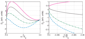
Figure 40: [color online] Plot of $\operatorname{Im}[D_{2}(\omega)]$ as a function of the frequency $\omega$ inside of the band gap for $m=0$, $r=10\,a$, $V=50\,\text{meV}$ and $\gamma_{1}=\gamma_{2}=\gamma$. Left: from top to bottom $\gamma=1.9,\,2.0,\,2.1,\,2.2$; Right: zoom in near the lower band edge, from top to bottom $\gamma=2.1,\,2.3,\,2.5,\,2.7$.

The important case of a screened Coulomb potential generally requires a different approach. Nevertheless, we do not anticipate any qualitative discrepancies between a potential well and a screened Coulomb potential. We expect the screening wave vector to be roughly proportional to the density of states at the Fermi energy; and once the range and the strength of the potential have been estimated a potential well can be used to approximate the binding energies. We also note that the asymptotic behavior in Eq. (78) is quite general for a decaying potential.

XIV.1 Polarization function

Since we were just discussing the issue of screening it fits well to briefly discuss the issue of the dielectric function in the biased bilayer (see also Ref. Stauber et al., 2007). With the introducing of the symmetric ($+$) and antisymmetric ($-$) densities (see e.g. Ref. [Nilsson et al., 2006b])

$$\rho_{\pm}({\bf q})=\sum_{{\bf k}}\psi^{{\dagger}}({\bf k}+{\bf q})\begin{pmatrix}1&0&0&0\\ 0&1&0&0\\ 0&0&\pm 1&0\\ 0&0&0&\pm 1\end{pmatrix}\psi({\bf k}).$$ (108)

The usual manipulations then gives the retarded response in the symmetric channel asGiuliani and Vignale (2005)

$$\chi_{++}(-{\bf q},\omega)=2\sum_{l,l^{\prime}}\int\frac{d{\bf k}}{(2\pi)^{2}}|v^{{\dagger}}_{l}({\bf k})v_{l^{\prime}}({\bf k}+{\bf q})|^{2}\\ \times\frac{n_{F}\bigl{[}E_{l}({\bf k})\bigr{]}-n_{F}\bigl{[}E_{l^{\prime}}({\bf k}+{\bf q})\bigr{]}}{E_{l}({\bf k})-E_{l^{\prime}}({\bf k}+{\bf q})+\omega+i\delta}.$$ (109)

Here $v_{l}({\bf k})$ is the spinor wave function of band $l$ at momentum ${\bf k}$. At half filling this expression only have contributions from $l\neq l^{\prime}$ and since the wave function overlap at ${\bf q}=0$ between different bands for a fixed value of ${\bf k}$ is zero we conclude that $\chi_{++}({\bf q},0)\propto q^{2}$ in the limit of $q\rightarrow 0$. The expression is expected to be dominated by the transitions between the $E_{-,-}$ and $E_{+,-}$-bands leading to $\chi_{++}({\bf q},0)\sim-2q^{2}/V$. The Random Phase Approximation (RPA) dielectric function is then given by $\epsilon({\bf q})\approx 1-(2\pi e^{2}/q)\chi_{++}({\bf q},0)$ which imply that $\epsilon({\bf q})\sim 1$ as $q\rightarrow 0$. From this we can conclude that the BGB is unable to contribute to the screening of the long-range part of the Coulomb interaction. Note that the dimensionality of the system is crucial for this argument. In three dimensions, where the Coulomb interaction goes as $1/q^{2}$, the same argument as in the above usually gives a large contribution to $\epsilon$ for a semiconductor.Ziman (1972) For the unbiased bilayer at $\mu=0$ in the low-energy approximation of Eq. (9) one finds (using RPA) a screening wave vector that is proportional to $t_{\perp}$.Nilsson et al. (2006b) This is in agreement with what one expects for an electron gas in 2D where the screening wave vector is proportional to the the effective mass. For a more detailed discussion of the unbiased graphene bilayer dielectric function including the trigonal warping see Ref. Wang and Chakraborty, 2007.

XV Coherent potential approximation

As discussed above in Sec. XII, for a finite density $n_{\rm i}$ of impurities, the bound states can interact with each other leading to the possibility of band gap renormalization and the formation of impurity bands. A simple, but crude, theory of these effects is the CPA.Soven (1967); Velický et al. (1968) In this approximation, the disorder is treated as a self-consistent medium with recovered translational invariance. The medium is described by a set of four local self-energies which are allowed to take on different values on all of the inequivalent lattice sites in the problem. In fact this section is a straightforward extension to the biased case of the methods applied in Sec. V for the unbiased case. The self-energies are chosen so that there is no scattering on average in the effective medium. It has been argued that the CPA is the best single-site approximation to the full solution of the problem.Velický et al. (1968)

In the following we often suppress the frequency dependence of the self-energies for brevity. The expression for the diagonal elements of the Green’s function ${\rm G}$ is given in App. D. We follow the standard approach to derive the CPA (see for example Refs. [Velický et al., 1968; Jones and March, 1985]), and we obtain the self-consistent equations:

$$\Sigma_{\alpha j}=\frac{n_{i}U}{1-(U-\Sigma_{\alpha j})\overline{{\rm G}}_{\alpha j}}.$$ (110)

The limit of site dilution (or vacancies) used in Sec. V is obtained in the limit $U\rightarrow\infty$ leading to the self-consistent equations:

$$\Sigma_{\alpha j}=-\frac{n_{i}}{\overline{\rm G}_{\alpha j}}.$$ (111)

An explicit expression for the local propagators $\overline{{\rm G}}_{\alpha j}$ is given in App. D. Using the expressions obtained there the self-consistent equations for $U\rightarrow\infty$ becomes:

$$\frac{n_{i}}{\Sigma_{\text{A}1}}=-\overline{{\rm G}}_{\text{A}1} = \beta_{1}(\xi_{1}-\alpha_{2}\beta_{2}\xi_{0}),$$ (112a)

$$\frac{n_{i}}{\Sigma_{\text{B}1}}=-\overline{{\rm G}}_{\text{B}1} = \alpha_{1}(\xi_{1}-\alpha_{2}\beta_{2}\xi_{0})+t_{\perp}^{2}\beta_{2}\xi_{0}.$$ (112b)

From these equations it is straightforward to obtain the density of states (DOS) on the different sublattices $\alpha j$ from $\rho_{\alpha j}(\omega)=-\operatorname{Im}\overline{\text{G}}_{\alpha j}(\omega+i\delta)/\pi$. In the clean case, one finds:

$$\rho_{\text{A}1}^{0} = \biggl{|}\frac{\omega-{V/2}}{2\Lambda^{2}}\biggl{[}\chi-\frac{\omega V(2-\chi)}{\sqrt{(V^{2}+t_{\perp}^{2})\omega^{2}-V^{2}t_{\perp}^{2}/4}}\biggr{]}\biggr{|},$$ (113a)

$$\rho_{\text{B}1}^{0} = \biggl{|}\rho_{\text{A}1}^{0}+\frac{t_{\perp}^{2}(\omega+{V/2})(2-\chi)}{2\Lambda^{2}\sqrt{(V^{2}+t_{\perp}^{2})\omega^{2}-V^{2}t_{\perp}^{2}/4}}\biggr{|},$$ (113b)

for $|\omega|\geq E_{\text{g}}/2$. Here $\chi=(0,1,2)$ for ($|\omega|\leq{V/2}$, ${V/2}\leq|\omega|\leq\sqrt{t_{\perp}^{2}+V^{2}/4}$, $\sqrt{t_{\perp}^{2}+V^{2}/4}\leq|\omega|$). The corresponding quantities in plane 2 are obtained by the substitution $V\rightarrow-V$. In the limit of $V\rightarrow 0$ we recover the known unbiased result of Eq. (28). Notice that the square-root singularity starts to appear already above $V/2$ on the B1 sublattice. There is also a divergence on the A1 sublattice but the coefficient in front is usually much smaller. The DOS on the A1 sublattice vanishes at $\omega=V/2$ while the DOS on the B1 sublattice is finite there.

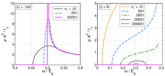
Figure 41: [color online] Left: DOS as a function of the energy (in units of $E_{g}$) close to the conduction band edge for different impurity concentrations (see inset), $U=-1$ eV. Right: Details of the DOS inside of the gap for different impurity concentrations for $U\to\infty$. In both cases $V=40\,\text{meV}$.

The numerically calculated density of states for $U\to\infty$ is shown in Fig. 41. The impurity band evolves from the single-impurity B$2$ bound state which for the parameters involved is located at $\epsilon\approx 0.3E_{\text{g}}$. Further evidence for this interpretation is that the total integrated DOS inside the split-off bands for the two lowest impurity concentrations is equal to $n_{i}$. It is worth mentioning that the width of the impurity band in the CPA is likely to be overestimated. The reason for this is that that the use of effective atoms, all of which have some impurity character, increases the interaction between the impurities.Velický et al. (1968) For smaller values of the impurity strength the single-impurity bound states are all weakly bound (cf. Fig. 37) and the “impurity bands” merge with the bulk bands as shown in Figs. 41 and 42. The bands have been shifted rigidly by the amount $n_{i}U$ for a more transparent comparison between the different cases. The smoothening of the singularity and the band gap renormalization is apparent. Observe also that the band edge moves further into the gap at the side where the bound states are located. It is likely that the CPA gives a better approximation for these states since by Eq. (79) they are weakly damped almost propagating modes. Notice that the gap and the whole structure of the DOS in the region of the gap is changing with $V$, and in particular the possibility that the actual gap closes before $V=0$ because of impurity-induced states inside of the gap. Finally we note that this observation is consistent with the results of numerically exact calculations using the recursive Green’s function method for strong disorder.Castro et al. (2007b)

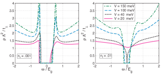
Figure 42: [color online] DOS as a function of energy (in units of $E_{g}$) for different values of the applied bias $V$ (see inset) and $U=-10$ eV. Left: $n_{i}=10^{-3}$; Right: $n_{i}=10^{-2}$.

XVI Effects of trigonal distortions

Before we conclude this paper we would like to briefly comment on the effect of the $\gamma_{3}$-term on our findings in the previous sections. The effects of $\gamma_{3}$ on the spectrum of the BGB was discussed in Sec. III, where it was shown that this term breaks the cylindrical symmetry and leads to the “trigonal distortion” of the bands. In the BGB the result is three copies of a more conventional elliptic dispersion at the lowest energies near the band edge. Using the same method as in Section XI we find that, also for an elliptical band edge, a Dirac delta potential always generates a bound state in 2D. The divergence of $\overline{{\rm G}}^{0}$ is generally only logarithmic as the band edge is approached however, whereas the divergence is an inverse square root without $\gamma_{3}$. More confined bound states with larger binding energies sample a larger area of the BZ. Therefore we do not expect that the small details at the band edge to significantly modify the results that we obtain with the minimal band model for these states.

Another observation is that when there is a finite density of impurities in the BGB the self-energies can become quite large as we have seen in the previous section. Consider the case $V=50\,\text{meV}$, for which $(V-E_{\text{g}})/E_{\text{g}}\approx 0.01$. Therefore, by looking at Fig. 5, we see that $\gamma_{3}$ smooth out the square-root singularity on this scale. Comparing with Fig. 41 we see that for an impurity of strength $U=-1\,\text{eV}$ the trigonal distortion would correspond to a density of impurities of around $n_{\rm i}\sim.001$. In the case that the gap is filled up with impurity-induced states (see Fig. 42), the disorder-induced energy scale is much larger than that generated by $\gamma_{3}$. Therefore we argue that the possibility that the gap closes before $V=0$ is robust to the presence of a $\gamma_{3}$, even if it is as large as the values quoted in the graphite literature.

XVII Conclusion and outlook

Graphene research is one of the fastest growing fields in condensed matter research since the isolation by Novoselov et al. of the first graphene flake in 2004.Novoselov et al. (2004) Three years after that, and after hundreds of theoretical papers on the subject,Castro Neto et al. (2007) the physics of single layer graphene is relatively well understood and very few controversies remain. Meanwhile, the study of multilayer graphene, and particularly bilayer graphene, continues to be, experimentally and theoretically, an open field of research. Partially, this can be assigned to the natural attraction of researchers to the “one atom thin” material and its unusual electronic spectra. Nevertheless, graphene bilayer is equally thin (two atoms thick, indeed) and has also 2D Dirac spectrum (albeit massive) with unusual properties. Graphene bilayer is also more prone to show strong electron-electron correlation effects, such as magnetism Nilsson et al. (2006b) and charge density wave Dahal et al. (b) phases, because of its finite density of states at the Dirac point, unlike its single layer counterpart where interactions are at most marginal in renormalization group sense.Peres et al. (2005) Interestingly enough, the study of the effect of electron-electron interactions in graphene is a field in its infancy.Kusminskiy et al. (2007); Min et al.

Furthermore, graphene bilayer is equally easy (or hard) to find or produce epitaxially. Besides its intriguing electronic properties, the graphene bilayer is a promising candidate to bulk electronic devices with properties that are insensitive to surface (edge) defects such as graphene nanoribbons and quantum dots. Perhaps even more interesting is the fact that graphene bilayer is the only known material that has an electronic gap between conduction and valence bands that can be fully controlled by the application of a transverse electric field (a tunable gap semiconductor), as has been demonstrated experimentally.Castro et al. (2007a); Oostinga et al. (2007) This property opens up an enormous number of possible ways to use bilayer graphene, from transistors to lasers working in the terahertz regime.

Nevertheless, in order to be able to use graphene bilayer (and multilayers) in device applications, one has to understand how material issues, such as disorder, affect its electronic properties. This was the main aim of this work, namely, to understand how disorder affects the electronic properties of bilayer (and multilayer) graphene in its most basic model. We have shown that the electronic self-energies can be calculated analytically within the T-matrix and CPA presenting some unusual features that can be measured either by transport or spectroscopy (ARPES and STM). We have calculated a series of important physical properties such as spectral functions, and frequency dependent conductivities. We have also studied the problem of bound states in the biased bilayer graphene and their effect in the electronic structure and have shown that the properties of these bound states can be equally well controlled by applied transverse fields. We also point that we have left open issues associated with trigonal distortions. At this point in time, it is not clear that such effects, associated with $\gamma_{3}$, are going to be the same as observed in 3D graphite and more experimental studies are needed in order to investigate the issue. We hope that our results will stimulate more experimental studies of these amazing new materials.

Appendix A Minimal conductivity of the graphene bilayer including trigonal warping

In this appendix we provide an alternative derivation of the value of the minimal conductivity of the graphene bilayer in the presence of trigonal warping. The conductance of a wide strip of graphene at the Dirac point is mediated by evanescent modes that connect the leads. We define the hamiltonian as

$${\cal H}\equiv\left(\begin{array}[]{cc}0&v_{F}(k_{x}+ik_{y})\\ v_{F}(k_{x}-ik_{y})&0\end{array}\right),$$ (114)

and use the Landauer formalism described in Refs. Katsnelson, 2006b; Tworzydlo et al., 2006. We take the width $W$ of the sample to be much larger than its length $L$. If we assume that the leads on the right and on the left are heavily doped clean graphene, the incoming, reflected, and outgoing waves can be approximated as:

$$\Psi_{in} \equiv \frac{1}{\sqrt{2}}\left(\begin{array}[]{c}1\\ 1\end{array}\right)e^{ik_{y}y},$$ (115c)

$$\Psi_{ref} \equiv \frac{r(k_{y})}{\sqrt{2}}\left(\begin{array}[]{c}1\\ -1\end{array}\right)e^{ik_{y}y},$$ (115f)

$$\Psi_{trans} \equiv \frac{t(k_{y})}{\sqrt{2}}\left(\begin{array}[]{c}1\\ 1\end{array}\right)e^{ik_{y}y},$$ (115i)

where $t(k_{y})$ [$r(k_{y})$] is the transmission [reflection] amplitude of the mode with perpendicular momentum $k_{y}$. The wavefunction in the central region, $0\leq x\leq L$, at zero energy, can be written as

$$\Psi\equiv A\left(\begin{array}[]{c}e^{-k_{y}x}\\ 0\end{array}\right)e^{ik_{y}y}+B\left(\begin{array}[]{c}0\\ e^{k_{y}x}\end{array}\right)e^{ik_{y}y}.$$ (116)

The matching conditions at the edges at $x=0$ and $x=L$ are:

$$1+r(k_{y}) = \sqrt{2}A,$$ (117a)

$$1-r(k_{y}) = \sqrt{2}B,$$ (117b)

$$t(k_{y}) = \sqrt{2}Ae^{-k_{y}L},$$ (117c)

$$t(k_{y}) = \sqrt{2}Be^{k_{y}L},$$ (117d)

resulting in the transmission probability

$$T(k_{y})\equiv|t(k_{y})|^{2}=\frac{1}{\cosh^{2}(k_{y}L)}.$$ (118)

The conductance per channel is thus given by

$$G=\frac{e^{2}}{h}\frac{W}{2\pi}\int_{-\infty}^{\infty}dk_{y}T(k_{y})=\Bigl{(}\frac{e^{2}}{\pi h}\Bigr{)}\frac{W}{L}.$$ (119)

We will now extend this result to the anisotropic Dirac equation. The Hamiltonian is

$${\cal H}\equiv\left(\begin{array}[]{cc}0&v_{x}k_{x}+iv_{y}k_{y}\\ v_{x}k_{k}-iv_{y}k_{y}&0\end{array}\right),$$ (120)

where the Fermi velocities ($v_{x}$ and $v_{y}$) are allowed to be different in the $x$ and $y$ directions. We use the incoming and outgoing wavefunctions wavefunctions in Eq. (115), and generalize the wavefunctions in the graphene junction, Eq. (116) to

$$\Psi\equiv A\left(\begin{array}[]{c}e^{-\kappa x}\\ 0\end{array}\right)e^{ik_{y}y}+B\left(\begin{array}[]{c}0\\ e^{\kappa x}\end{array}\right)e^{ik_{y}y},$$ (121)

where the Dirac equation implies that $\kappa=v_{y}k_{y}/v_{x}$. Matching the wave functions at the contacts with the leads, we find that the generalization of Eq. (118) is

$$T(k_{y})=\frac{1}{\cosh^{2}\left(\frac{v_{y}k_{y}L}{v_{x}}\right)},$$ (122)

so that

$$G=\Bigl{(}\frac{e^{2}}{\pi h}\Bigr{)}\Bigl{(}\frac{v_{x}}{v_{y}}\Bigr{)}\frac{W}{L}.$$ (123)

If the junction is rotated by an angle $\theta$ with respect to the main axes of the anisotropic Dirac equation, the Hamiltonian becomes:

$${\cal H}\equiv\left(\begin{array}[]{cc}0&v_{a}[k_{x}\cos(\theta)-k_{y}\sin(\theta)]+iv_{b}[k_{x}\sin(\theta)+k_{y}\cos(\theta)]\\ v_{a}[k_{x}\cos(\theta)-k_{y}\sin(\theta)]-iv_{b}[k_{x}\sin(\theta)+k_{y}\cos(\theta)]&0\end{array}\right),$$ (124)

where $v_{a}$ and $v_{b}$ are the Fermi velocities along the two principal axes. The wave function in the central region is now

$$\Psi\equiv A\left(\begin{array}[]{c}e^{-\kappa x}e^{ik^{\prime}x}\\ 0\end{array}\right)e^{ik_{y}y}+B\left(\begin{array}[]{c}0\\ e^{\kappa x}e^{ik^{\prime}x}\end{array}\right)e^{ik_{y}y},$$ (125)

where

$$\kappa = \frac{v_{a}v_{b}}{v_{a}^{2}\cos^{2}(\theta)+v_{b}^{2}\sin^{2}(\theta)}k_{y},$$ (126a)

$$k^{\prime} = \frac{\sin(\theta)\cos(\theta)(v_{a}^{2}-v_{b}^{2})}{v_{a}^{2}\cos^{2}(\theta)+v_{b}^{2}\sin^{2}(\theta)}k_{y}.$$ (126b)

Using this we also obtain

$$T(k_{y})=\frac{1}{\cosh^{2}\left(\frac{v_{a}v_{b}k_{y}L}{v_{a}\cos^{2}(\theta)+v_{b}^{2}\sin^{2}(\theta)}\right)},$$ (127)

leading to

$$G=\Bigl{(}\frac{e^{2}}{\pi h}\Bigr{)}\Bigl{(}\frac{v_{a}^{2}\cos^{2}(\theta)+v_{b}^{2}\sin^{2}(\theta)}{v_{a}v_{b}}\Bigr{)}\frac{W}{L}.$$ (128)

In a graphene bilayer, including trigonal warping but ignoring terms that couple sites in the same sublattice, we have four Dirac points. One of them is isotropic, with $v_{a}=v_{b}$, and the three others are anisotropic, with $v_{b}=3v_{a}$. The principal axes at these three Dirac points form angles with respect to a barrier which can be parametrized as $\theta_{0},\theta_{0}+2\pi/3$ and $\theta_{0}+4\pi/3$, where $\theta_{0}$ depends on the orientation of the barrier. The conductance is therefore given by

$$G=\Bigl{(}\frac{e^{2}}{\pi h}\Bigr{)}\frac{W}{L}\left[1+\frac{3}{2}\left(\frac{v_{a}}{v_{b}}+\frac{v_{b}}{v_{a}}\right)\right].$$ (129)

This expression is independent of the angle $\theta_{0}$. For $v_{b}/v_{a}=3$, we find $G=6\times[e^{2}/(\pi h)]\times(W/L)$ per channel, in agreement with Refs. Koshino and Ando, 2006; Cserti et al., 2007.

Appendix B Density of states in multilayer graphene

In this appendix we derive explicit expressions for the DOS in graphene multilayers. The expressions are used in Section VI. To calculate the DOS in graphite we must perform two integrals to get $\overline{{\rm G}}$. One integral we need is

$$I_{1}=\int_{0}^{\Lambda^{2}}d(p^{2})\int_{-\pi/2}^{\pi/2}\frac{dk_{\perp}}{\pi}\Bigl{[}\frac{1}{2D_{-}}+\frac{1}{2D_{+}}\Bigr{]}.$$ (130)

First we perform the perpendicular integral using complex variables to rewrite the integral as a contour integral around the unit circle and then picking up the pole inside:

$$\int_{-\pi/2}^{\pi/2}dk_{\perp}\Bigl{[}\frac{1}{D_{-}}+\frac{1}{D_{+}}\Bigr{]}\\ =\frac{1}{\omega-\Sigma_{B}}\oint\frac{dz}{i}\frac{1}{t_{\perp}(z^{2}+1)-Az}\\ =-\frac{2\pi}{\omega-\Sigma_{B}}\frac{\operatorname{sign}[\operatorname{Re}(A)]}{\sqrt{A^{2}-4t_{\perp}^{2}}},$$

where $A\equiv p^{2}/(\omega-\Sigma_{B})-(\omega-\Sigma_{A})$. Note that the function $\operatorname{sign}[\operatorname{Re}(A)]$ changes sign just where the branch of the square root does. Moreover the square root is purely imaginary there. Therefore the function is actually continuous across the point where $\operatorname{Re}(A)=0$. From now on in this appendix, as well as in Appendix C.2, we choose the branch of the square root such that the sign of the real part is included, with this convention $A$ and $\sqrt{A^{2}-4t_{\perp}^{2}}$ always lies in the same quadrant of the complex plane. Because of the form of $A$ we can use the integral formula

$$\xi^{(1)}(p^{2})=\int d(p^{2})\frac{1}{\sqrt{A^{2}-4t_{\perp}^{2}}}\\ =(\omega-\Sigma_{B})\log\Bigl{[}A+\sqrt{A^{2}-4t_{\perp}^{2}}\Bigr{]},$$ (131)

directly, since the argument of the log does not cross any branch cut. Thus the result of the integral is

$$I_{1}=-\log\Bigl{[}\frac{A(\Lambda^{2})+\sqrt{A^{2}(\Lambda^{2})-4t_{\perp}^{2}}}{A(0)+\sqrt{A^{2}(0)-4t_{\perp}^{2}}}\Bigr{]}.$$ (132)

Finally to leading order in $\Lambda$ we get

$$I_{1}=-\log\Bigl{[}\frac{2\Lambda^{2}}{-(\omega-\Sigma_{\text{B}})(\omega-\Sigma_{\text{A}}+\sqrt{(\omega-\Sigma_{\text{A}})^{2}-4t_{\perp}^{2}}}\Bigr{]}.$$ (133)

Similarly the integral

$$I_{2}=\int_{0}^{\Lambda^{2}}d(p^{2})\int_{-\pi/2}^{\pi/2}\frac{dk}{\pi}\Bigl{[}\frac{-2t_{\perp}\cos(k)}{2D_{-}}+\frac{2t_{\perp}\cos(k)}{2D_{+}}\Bigr{]},$$ (134)

can be written as

$$I_{2}=\frac{1}{\omega-\Sigma_{B}}\Bigl{[}\Lambda^{2}-\int_{0}^{\Lambda^{2}}d(p^{2})\frac{A}{\sqrt{A^{2}-4t_{\perp}^{2}}}\Bigr{]}.$$ (135)

Now we may use the integral formula

$$\int d(p^{2})\frac{A}{\sqrt{A^{2}-4t_{\perp}^{2}}}=(\omega-\Sigma_{B})\sqrt{A^{2}-4t_{\perp}^{2}}\bigr{)},$$ (136)

and one can once again convince oneself that there are no contribution from the possible crossing of the branch at $\operatorname{Re}(A)=0$. With the help of this the resulting expression becomes

$$I_{2}=\frac{1}{\omega-\Sigma_{B}}\Bigl{\{}\Lambda^{2}-(\omega-\Sigma_{B})\Bigl{[}\sqrt{A^{2}(\Lambda^{2})-4t_{\perp}^{2}}\\ +\sqrt{A^{2}(0)-4t_{\perp}^{2}}\Bigl{]}\Bigr{\}}.$$ (137)

Finally, keeping only the leading term in the expansion in $\Lambda$ we get

$$I_{2}=(\omega-\Sigma_{A})-\sqrt{(\omega-\Sigma_{A})^{2}-4t_{\perp}^{2}}.$$ (138)

Appendix C Conductivity kernels

In this appendix we derive formulas for the conductivity kernels that we use in Sec. VIII and Sec. IX. First we rewrite the kernels with the identity

$$\operatorname{Im}\bigl{[}{\rm G}_{1}(\epsilon)\bigr{]}\operatorname{Im}\bigl{[}{\rm G}_{2}(\epsilon+\omega)\bigr{]}\\ =\frac{1}{2}\operatorname{Re}\bigl{[}{\rm G}_{1}^{A}(\epsilon){\rm G}_{2}^{R}(\epsilon+\omega)-{\rm G}_{1}^{R}(\epsilon){\rm G}_{2}^{R}(\epsilon+\omega)\bigr{]}\\ =\frac{1}{2}\operatorname{Re}\Bigl{[}\sum_{\gamma=\pm}\gamma{\rm G}_{1}(E_{1}-i\gamma\Gamma_{1}){\rm G}_{2}(E_{2}+i\Gamma_{2})\Bigr{]},$$ (139)

and introduce the notations

$$E_{A} = \epsilon-\Sigma_{\text{A}}(\epsilon),$$ (140a)

$$E_{B} = \epsilon-\Sigma_{\text{B}}(\epsilon),$$ (140b)

$$\widetilde{E}_{A} = \epsilon+\omega-\Sigma_{\text{A}}(\epsilon+\omega),$$ (140c)

$$\widetilde{E}_{B} = \epsilon+\omega-\Sigma_{\text{B}}(\epsilon+\omega).$$ (140d)

C.1 Bilayer graphene

The integrals we need for the bilayer are easy to obtain since there is never any problems with branches of the logarithms. The kernels can be expressed in terms of the following integrals:

$$\int_{0}^{\Lambda^{2}}d(p^{2}){\rm g_{AA}^{D}}(\epsilon){\rm g_{BB}^{D}}(\epsilon+\omega)=\frac{1}{4}\sum_{\alpha,\beta}\frac{E_{B}(\widetilde{E}_{A}+\beta t_{\perp})}{E_{B}(E_{A}+\alpha t_{\perp})-\widetilde{E}_{B}(\widetilde{E}_{A}+\beta t_{\perp})}\log\Bigl{[}\frac{-\widetilde{E}_{B}(\widetilde{E}_{A}+\beta t_{\perp})}{-E_{B}(E_{A}+\alpha t_{\perp})}\Bigl{]},$$ (141)

$$\int_{0}^{\Lambda^{2}}d(p^{2}){\rm g_{BB}^{D}}(\epsilon){\rm g_{AA}^{D}}(\epsilon+\omega)=\frac{1}{4}\sum_{\alpha,\beta}\frac{\widetilde{E}_{B}(E_{A}+\alpha t_{\perp})}{\widetilde{E}_{B}(\widetilde{E}_{A}+\beta t_{\perp})-E_{B}(E_{A}+\alpha t_{\perp})}\log\Bigl{[}\frac{-E_{B}(E_{A}+\alpha t_{\perp})}{-\widetilde{E}_{B}(\widetilde{E}_{A}+\beta t_{\perp})}\Bigl{]},$$ (142)

$$\int_{0}^{\Lambda^{2}}d(p^{2}){\rm g_{AB}^{ND}}(\epsilon){\rm g_{AB}^{ND}}(\epsilon+\omega)=\frac{1}{4}\sum_{\alpha,\beta}\frac{\alpha\beta}{E_{B}(E_{A}+\alpha t_{\perp})-\widetilde{E}_{B}(\widetilde{E}_{A}+\beta t_{\perp})}\times\\ \Bigl{\{}E_{B}(E_{A}+\alpha t_{\perp})\log\Bigl{[}\frac{\Lambda^{2}}{-E_{B}(E_{A}+\alpha t_{\perp})}\Bigr{]}-\widetilde{E}_{B}(\widetilde{E}_{A}+\beta t_{\perp})\log\Bigl{[}\frac{\Lambda^{2}}{-\widetilde{E}_{B}(\widetilde{E}_{A}+\beta t_{\perp})}\Bigr{]}\Bigl{\}},$$ (143)

and

$$\int_{0}^{\Lambda^{2}}d(p^{2})\bigl{[}{\rm g_{AA}^{D}}(\epsilon){\rm g_{AA}^{D}}(\epsilon+\omega)-{\rm g_{AA}^{ND}}(\epsilon){\rm g_{AA}^{ND}}(\epsilon+\omega)\bigr{]}\\ =\frac{1}{2}\sum_{\alpha}\frac{E_{B}\widetilde{E}_{B}}{E_{B}(E_{A}+\alpha t_{\perp})-\widetilde{E}_{B}(\widetilde{E}_{A}-\alpha t_{\perp})}\log\Bigl{[}\frac{-\widetilde{E}_{B}(\widetilde{E}_{A}-\alpha t_{\perp})}{-E_{B}(E_{A}+\alpha t_{\perp})}\Bigl{]}.$$ (144)

In fact, although the cutoff $\Lambda$ enter the expression in Eq. (143), the final result is actually independent of $\Lambda$. For the DC conductivity it is convenient to work out that for two retarded propagators we have the relation

$$\int_{0}^{\Lambda^{2}}d(p^{2})\bigl{[}{\rm g_{AA}^{D}}(\epsilon){\rm g_{BB}^{D}}(\epsilon)+{\rm g_{AB}^{ND}}(\epsilon){\rm g_{AB}^{ND}}(\epsilon)\bigr{]}=-1.$$ (145)

C.2 Multilayer graphene

For multilayer graphene we have to perform two integrals, they are

$$J_{1}=\int_{0}^{\Lambda^{2}}d(p^{2})\int_{-\pi/2}^{\pi/2}\frac{dk}{\pi}\bigl{[}{\rm g_{AA}^{D}}\widetilde{\rm g_{BB}^{D}}+{\rm g_{BB}^{D}}\widetilde{\rm g_{AA}^{D}}+2{\rm g_{AB}^{ND}}\widetilde{\rm g_{AB}^{ND}}\bigr{]},$$ (146)

and

$$J_{2}=\int_{0}^{\Lambda^{2}}d(p^{2})\int_{-\pi/2}^{\pi/2}\frac{dk}{\pi}\bigl{[}{\rm g_{AA}^{D}}\widetilde{\rm g_{AA}^{D}}+{\rm g_{AA}^{ND}}\widetilde{\rm g_{AA}^{ND}}\bigr{]}\sin^{2}(k).$$ (147)

Exactly like in the case above we find $J_{1}=-2$ when $\omega=0$ and both the propagators are retarded. First we perform the perpendicular integral using a contour integral as we did when we computed the DOS in Appendix B. In the following the branch of the square root includes the sign of the real part $\sqrt{A^{2}-4t_{\perp}^{2}}\equiv\operatorname{sign}[\operatorname{Re}(A)]\sqrt{A^{2}-4t_{\perp}^{2}}$. This implies that $A$ and $\sqrt{A^{2}-4t_{\perp}^{2}}$ always lies in the same quadrant. The results we need are

$$\int_{-\pi/2}^{\pi/2}\frac{dk}{\pi}{\rm g_{AA}^{D}}(\epsilon){\rm g_{BB}^{D}}(\epsilon+\omega)=-\frac{1}{2\widetilde{E}_{B}}\biggl{\{}\frac{2}{\sqrt{A^{2}-4t_{\perp}^{2}}}\\ +\frac{p^{2}}{\widetilde{E}_{B}}\Bigl{[}\frac{1}{A-\widetilde{A}}-\frac{1}{A+\widetilde{A}}\Bigl{]}\frac{1}{\sqrt{A^{2}-4t_{\perp}^{2}}}+\frac{p^{2}}{\widetilde{E}_{B}}\Bigl{[}\frac{1}{\widetilde{A}-A}-\frac{1}{A+\widetilde{A}}\Bigl{]}\frac{1}{\sqrt{\widetilde{A}^{2}-4t_{\perp}^{2}}}\biggr{\}},$$ (148)

$$\int_{-\pi/2}^{\pi/2}\frac{dk}{\pi}{\rm g_{AB}^{ND}}(\epsilon){\rm g_{AB}^{ND}}(\epsilon+\omega)=-\frac{p^{2}}{2E_{B}\widetilde{E}_{B}}\Bigl{\{}\Bigl{[}\frac{1}{A-\widetilde{A}}+\frac{1}{A+\widetilde{A}}\Bigr{]}\frac{1}{\sqrt{A^{2}-4t_{\perp}^{2}}}+\Bigl{[}\frac{1}{\widetilde{A}-A}+\frac{1}{A+\widetilde{A}}\Bigr{]}\frac{1}{\sqrt{\widetilde{A}^{2}-4t_{\perp}^{2}}}\Bigr{\}},$$ (149)

and

$$\int_{-\pi/2}^{\pi/2}\frac{dk}{\pi}\bigl{[}{\rm g_{AA}^{D}}(\epsilon){\rm g_{AA}^{D}}(\epsilon+\omega)+{\rm g_{AA}^{ND}}(\epsilon){\rm g_{AA}^{ND}}(\epsilon+\omega)\bigr{]}\sin^{2}(k)\\ =\frac{1}{4t_{\perp}^{2}}\Bigl{\{}-1+\frac{1}{A-\widetilde{A}}\Bigr{[}\sqrt{A^{2}-4t_{\perp}^{2}}-\sqrt{\widetilde{A}^{2}-4t_{\perp}^{2}}\Bigr{]}.$$ (150)

Where

$$A = p^{2}/E_{B}-E_{A},$$ (151)

$$\widetilde{A} = p^{2}/\widetilde{E}_{B}-\widetilde{E}_{A}.$$ (152)

Adding up all the contributions for the $J_{1}$ we get after some rearrangements

$$J_{1}=\int_{0}^{\Lambda^{2}}d(p^{2})\biggl{\{}-\Bigl{[}\frac{1}{\widetilde{E}_{B}}\frac{1}{\sqrt{A^{2}-4t_{\perp}^{2}}}+\frac{1}{E_{B}}\frac{1}{\sqrt{\widetilde{A}^{2}-4t_{\perp}^{2}}}\Bigr{]}+\frac{d_{-}^{2}}{2d_{+}}\Bigl{[}1+\frac{c_{+}}{p^{2}-c_{+}}\Bigr{]}\times\Bigl{[}\frac{1}{\sqrt{A^{2}-4t_{\perp}^{2}}}+\frac{1}{\sqrt{\widetilde{A}^{2}-4t_{\perp}^{2}}}\Bigr{]}\\ -\frac{d_{+}^{2}}{2d_{-}}\Bigl{[}1+\frac{c_{-}}{p^{2}-c_{-}}\Bigr{]}\times\Bigl{[}\frac{1}{\sqrt{A^{2}-4t_{\perp}^{2}}}-\frac{1}{\sqrt{\widetilde{A}^{2}-4t_{\perp}^{2}}}\Bigr{]}\biggr{\}},$$ (153)

where

$$c_{\pm} = \frac{E_{A}\pm\widetilde{E}_{A}}{d_{\pm}}=E_{B}\widetilde{E}_{B}\frac{E_{A}\pm\widetilde{E}_{A}}{\widetilde{E}_{B}\pm E_{B}}$$ (154)

$$d_{\pm} = \frac{1}{E_{B}}\pm\frac{1}{\widetilde{E}_{B}}=\frac{\widetilde{E}_{B}\pm E_{B}}{E_{B}\widetilde{E}_{B}}.$$ (155)

It is convenient to define the integral

$$\xi_{\pm}^{(2)}(p^{2})=\int d(p^{2})\frac{1}{p^{2}-c_{\pm}}\frac{1}{\sqrt{A^{2}-4t_{\perp}^{2}}}\\ =\frac{1}{\sqrt{B_{\pm}^{2}-4t_{\perp}^{2}}}\Bigl{\{}\log(p^{2}-c_{\pm})-\log\bigl{[}AB_{\pm}+\sqrt{A^{2}-4t_{\perp}^{2}}\sqrt{B_{\pm}^{2}-4t_{\perp}^{2}}-4t_{\perp}^{2}\bigl{]}\Bigl{\}},$$ (156)

in which we have introduced

$$B_{\pm}=c_{\pm}/E_{B}-E_{A},$$ (157)

and the square roots are again chosen such that $B_{\pm}$ and $\sqrt{B_{\pm}^{2}-4t_{\perp}^{2}}$ are in the same quadrant in the complex plane. Using this we may write

$$\int d(p^{2})\frac{1}{p^{2}-c_{\pm}}\sqrt{A^{2}-4t_{\perp}^{2}}=\sqrt{A^{2}-4t_{\perp}^{2}}+B_{\pm}\log\bigl{[}A+\sqrt{A^{2}-4t_{\perp}^{2}}\bigl{]}+\bigl{[}B_{\pm}^{2}-4t_{\perp}^{2}\bigr{]}\xi_{\pm}^{(2)}(p^{2}),$$ (158)

If we use this formulas blindly and just plug in the endpoints the resulting expressions are

$$J_{1}=\biggl{\{}\Bigl{[}\frac{d_{-}^{2}}{2d_{+}}-\frac{d_{+}^{2}}{2d_{-}}-\frac{1}{\widetilde{E}_{B}}\Bigl{]}\xi^{(1)}(z)+\Bigl{[}\frac{d_{-}^{2}}{2d_{+}}+\frac{d_{+}^{2}}{2d_{-}}-\frac{1}{E_{B}}\Bigl{]}\widetilde{\xi}^{(1)}(z)\\ +\frac{d_{-}^{2}c_{+}}{2d_{+}}\Bigl{[}\xi_{+}^{(2)}(z)+\widetilde{\xi}_{+}^{(2)}(z)\Bigr{]}-\frac{d_{+}^{2}c_{-}}{2d_{-}}\Bigl{[}\xi_{-}^{(2)}(z)-\widetilde{\xi}_{-}^{(2)}(z)\Bigr{]}\biggl{\}}_{0}^{\Lambda^{2}},$$ (159)

and

$$J_{2}=\frac{1}{4t_{\perp}^{2}}\Bigl{\{}-z+\frac{1}{d_{-}}\Bigl{[}\sqrt{A^{2}-4t_{\perp}^{2}}-\sqrt{\widetilde{A}^{2}-4t_{\perp}^{2}}+\frac{B_{-}}{E_{B}}\xi^{(1)}(z)-\frac{\widetilde{B}_{-}}{\widetilde{E}_{B}}\widetilde{\xi}^{(1)}(z)\\ +\bigl{[}B_{-}^{2}-4t_{\perp}^{2}\bigr{]}\xi_{-}^{(2)}(z)-\bigl{[}\widetilde{B}_{-}^{2}-4t_{\perp}^{2}\bigr{]}\widetilde{\xi}_{-}^{(2)}(z)\Bigl{]}\biggl{\}}_{z=0}^{\Lambda^{2}}.$$ (160)

One must be careful with the imaginary part of $\xi^{(2)}$ however. First we note that $\widetilde{B}_{+}=-B_{+}$ and $\widetilde{B}_{-}=B_{-}$, which implies that the $\log(p^{2}-c_{\pm})$ term in $\xi^{(2)}$ does not contribute. Secondly, we write $A=2t_{\perp}\cosh(\alpha)$ and $B=2t_{\perp}\cosh(\beta)$ and use hyperbolic trigonometric identities to write:

$$\log\Bigl{[}AB+\sqrt{A^{2}-4t_{\perp}^{2}}\sqrt{B^{2}-4t_{\perp}^{2}}-4t_{\perp}^{2}\Bigr{]}\\ =\log\{4t_{\perp}^{2}[\cosh(\alpha+\beta)-1]\}\\ =\log(8t_{\perp}^{2})+2\log\Bigl{[}\sinh\Bigl{(}\frac{\alpha+\beta}{2}\Bigr{)}\Bigr{]}.$$ (161)

By convention $\operatorname{Re}(\alpha)>0$ and $-\pi\leq\operatorname{Im}(\alpha)<\pi$ (and the same goes for $\beta$). Therefore $-\pi<\operatorname{Im}(\alpha+\beta)/2<\pi$ and the argument of the log never crosses the branch cut along the negative real axis. Therefore the representation of $A$ and $B$ in terms of hyperbolic functions automatically takes care of the phase information of the argument. Finally, the case when $B$ is purely real and negative (this is relevant for the calculation of the DC conductivity) requires that one should choose $\operatorname{Im}(\beta)<0$ so that $\operatorname{sign}[\operatorname{Re}(B)]\sqrt{B^{2}-4t_{\perp}^{2}}=2t_{\perp}\sinh(\beta)$.

Appendix D Local propagator in the biased graphene bilayer

In this appendix we provide some details on the calculation of the local propagator in the BGB that we use in Sec. XV. Introducing the notations:

$$\alpha_{1} = \omega-V/2-\Sigma_{\text{A}1},$$ (162a)

$$\beta_{1} = \omega-V/2-\Sigma_{\text{B}1},$$ (162b)

$$\alpha_{2} = \omega+V/2-\Sigma_{\text{A}2},$$ (162c)

$$\beta_{2} = \omega+V/2-\Sigma_{\text{B}2},$$ (162d)

one can write

$${\rm G}_{\text{A}1\text{A}1} = \frac{\beta_{1}(\alpha_{2}\beta_{2}-k^{2})}{D},$$ (163a)

$${\rm G}_{\text{B}1\text{B}1} = \frac{\alpha_{1}(\alpha_{2}\beta_{2}-k^{2})-t_{\perp}^{2}\beta_{2}}{D}.$$ (163b)

The equations for the corresponding quantities in layer 2 are obtained by exchanging the indeces $1\leftrightarrow 2$ everywhere. The denominator can be written as

$$D=(\alpha_{1}\beta_{1}-k^{2})(\alpha_{2}\beta_{2}-k^{2})-t_{\perp}^{2}\beta_{1}\beta_{2}\equiv(k^{2}-z_{-})(k^{2}-z_{+}),$$ (164)

where we have defined

$$z_{\pm}=\frac{\alpha_{1}\beta_{1}+\alpha_{2}\beta_{2}}{2}\pm\frac{1}{2}\sqrt{(\alpha_{1}\beta_{1}-\alpha_{2}\beta_{2})^{2}+4t_{\perp}^{2}\beta_{1}\beta_{2}}.$$ (165)

Introducing the integrals

$$\Lambda^{2}\xi_{0}=\int_{0}^{\Lambda^{2}}d(k^{2})\frac{1}{D}\\ =\frac{1}{z_{+}-z_{-}}\Bigl{[}\ln\Bigl{(}\frac{\Lambda^{2}-z_{+}}{-z_{+}}\Bigr{)}-\ln\Bigl{(}\frac{\Lambda^{2}-z_{-}}{-z_{-}}\Bigr{)}\Bigr{]}\\ \approx\frac{1}{z_{+}-z_{-}}\Bigl{[}\ln\Bigl{(}\frac{\Lambda^{2}}{-z_{+}}\Bigr{)}-\ln\Bigl{(}\frac{\Lambda^{2}}{-z_{-}}\Bigr{)}\Bigr{]},$$ (166)

and

$$\Lambda^{2}\xi_{1}=\int_{0}^{\Lambda^{2}}d(k^{2})\frac{k^{2}}{D}\\ =\frac{1}{z_{+}-z_{-}}\Bigl{[}z_{+}\ln\Bigl{(}\frac{\Lambda^{2}-z_{+}}{-z_{+}}\Bigr{)}-z_{-}\ln\Bigl{(}\frac{\Lambda^{2}-z_{-}}{-z_{-}}\Bigr{)}\Bigr{]}\\ \approx\frac{1}{z_{+}-z_{-}}\Bigl{[}z_{+}\ln\Bigl{(}\frac{\Lambda^{2}}{-z_{+}}\Bigr{)}-z_{-}\ln\Bigl{(}\frac{\Lambda^{2}}{-z_{-}}\Bigr{)}\Bigr{]},$$ (167)

we can easily compute $\overline{\text{G}}$. Using the explicit form of the propagators in Eq. (163) and the same continuum approximation as in Eq. (25) we obtain

$$-\overline{{\rm G}}_{\text{A}1} = \beta_{1}(\xi_{1}-\alpha_{2}\beta_{2}\xi_{0}),$$ (168a)

$$-\overline{{\rm G}}_{\text{B}1} = \alpha_{1}(\xi_{1}-\alpha_{2}\beta_{2}\xi_{0})+t_{\perp}^{2}\beta_{2}\xi_{0}.$$ (168b)

Again the corresponding quantities in plane 2 are obtained by exchanging the indeces $1\leftrightarrow 2$ everywhere.

References

- Novoselov et al. (2004) K. S. Novoselov, A. K. Geim, S. V. Morozov, D. Jiang, Y. Zhang, S. V. Dubonos, I. V. Gregorieva, and A. A. Firsov, Science 306, 666 (2004).
- Castro Neto et al. (2006) A. H. Castro Neto, F. Guinea, and N. M. R. Peres, Physics World 19, 33 (2006).
- Castro Neto et al. (2007) A. H. Castro Neto, F. Guinea, N. M. R. Peres, K. S. Novoselov, and A. K. Geim (2007), arXiv:0709.1163.
- Geim and Novoselov (2007) A. K. Geim and K. S. Novoselov, Nature Materials 6, 183 (2007).
- Berger et al. (2004) C. Berger, Z. M. Song, T. B. Li, X. B. Li, A. Y. Ogbazghi, R. Feng, Z. T. Dai, A. N. Marchenkov, E. H. Conrad, P. N. First, et al., J. Phys. Chem. B 108, 19912 (2004).
- Nakada et al. (1996) K. Nakada, M. Fujita, G. Dresselhaus, and M. S. Dresselhaus, Phys. Rev. B 54, 17954 (1996).
- Silvestrov and Efetov (2007) P. G. Silvestrov and K. B. Efetov, Phys. Rev. Lett. 98, 016802 (2007).
- Han et al. (2007) M. Y. Han, B. Özyilmaz, Y. Zhang, and P. Kim, Phys. Rev. Lett. 98, 206805 (2007).
- Sols et al. (2007) F. Sols, F. Guinea, and A. H. Castro Neto, Phys. Rev. Lett. 99, 166803 (2007).
- McCann and Fal’ko (2006) E. McCann and V. I. Fal’ko, Phys. Rev. Lett. 96, 086805 (2006).
- McCann (2006) E. McCann, Phys. Rev. B 74, 161403 (2006).
- Oostinga et al. (2007) J. B. Oostinga, H. B. Heersche, X. Liu, A. F. Morpurgo, and L. M. K. Vandersypen, Nature Mat. online 10.1038, nmat2082 (2007).
- Castro et al. (2007a) E. V. Castro, K. S. Novoselov, S. V. Morozov, N. M. R. Peres, J. M. B. L. dos Santos, J. Nilsson, F. Guinea, A. K. Geim, and A. H. C. Neto, Phys. Rev. Lett. 99, 216802 (2007a).
- J. Milton Pereira et al. (2007) J. J. Milton Pereira, P. Vasilopoulos, and F. M. Peeters, Nano Lett. 7, 946 (2007).
- Nilsson et al. (2007) J. Nilsson, A. H. Castro Neto, F. Guinea, and N. M. R. Peres, Phys. Rev. B 76, 165416 (2007).
- Peres et al. (2006) N. M. R. Peres, F. Guinea, and A. H. Castro Neto, Phys. Rev. B 73, 125411 (2006).
- Nilsson et al. (2006a) J. Nilsson, A. H. Castro Neto, F. Guinea, and N. M. R. Peres, Phys. Rev. Lett. 97, 266801 (2006a).
- Nilsson and Castro Neto (2007) J. Nilsson and A. H. Castro Neto, Phys. Rev. Lett. 98, 126801 (2007).
- Katsnelson (2007) M. I. Katsnelson, Phys. Rev. B 76, 073411 (2007).
- (20) S. Adam and S. D. Sarma, arXiv:0711.0003v3 (unpublished).
- Kechedzhi et al. (2007) K. Kechedzhi, V. I. Fal’ko, E. McCann, and B. L. Altshuler, Phys. Rev. Lett. 98, 176806 (2007).
- (22) S. Morozov, K. Novoselov, M. Katsnelson, F. Schedin, D. Elias, J. Jaszczak, and A. Geim, arXiv:0710.5304v1 (unpublished).
- Gorbachev et al. (2007) R. V. Gorbachev, F. V. Tikhonenko, A. S. Mayorov, D. W. Horsell, and A. K. Savchenko, Phys. Rev. Lett. 98, 176805 (2007).
- (24) M. Nakamura and L. Hirasawa, arXiv:0711.2940v1 (to be published).
- (25) This approximation gives a good account of the electronic properties as long as the localization length is larger than the sample size. This condition is not constraining in 2D due to the exponetially large localization length.
- Ziegler (2006) K. Ziegler, Phys. Rev. Lett. 97, 266802 (2006).
- Zhou et al. (2006a) S. Y. Zhou, G.-H. Gweon, J. Graf, A. V. Fedorov, C. D. Spataru, R. D. Diehl, Y. Kopelevich, D.-H. Lee, S. G. Louie, and A. Lanzara, Nature Physics 2, 595 (2006a).
- Zhou et al. (2006b) S. Y. Zhou, G. H. Gweon, and A. Lanzara, Annals of Physics 321, 1730 (2006b).
- Bostwick et al. (2007) A. Bostwick, T. Ohta, T. Seyller, K. Horn, and E. Rotenberg, Nature Physics 3, 36 (2007).
- Ohta et al. (2006) T. Ohta, A. Bostwick, T. Seyller, K. Horn, and E. Rotenberg, Science 313, 951 (2006).
- Zhou et al. (2007) S. Y. Zhou, G.-H. Gweon, A. V. Fedorov, P. N. First, W. A. der Heer, D.-H. Lee, F. Guinea, A. H. Castro Neto, and A. Lanzara, Nature Mat. 6, 770 (2007).
- Stolyarova et al. (2007) E. Stolyarova, K. T. Rim, S. Ryu, J. Maultzsch, P. Kim, L. E. Brus, T. F. Heinz, M. S. Hybertsen, and G. W. Flynn, Proceedings of the National Academy of Sciences 104, 9209 (2007).
- Mallet et al. (2007) P. Mallet, F. Varchon, C. Naud, L. Magaud, C. Berger, and J.-Y. Veuillen, Phys. Rev. B 76, 041403 (2007).
- Li and Andrei (2007) G. Li and E. V. Andrei, Nature Physics 3, 623 (2007).
- Brar et al. (2007) V. W. Brar, Y. Zhang, Y. Yayon, T. Ohta, J. L. McChesney, A. Bostwick, E. Rotenberg, K. Horn, and M. F. Crommie, Appl. Phys. Lett. 91, 122102 (2007).
- Brandt et al. (1988) N. B. Brandt, S. M. Chudinov, and Y. G. Ponomarev, Semimetals 1: Graphite and its Compounds (North-Holland (Amsterdam), 1988).
- McClure (1957) J. W. McClure, Phys. Rev. 108, 612 (1957).
- Slonczewski and Weiss (1958) J. C. Slonczewski and P. R. Weiss, Phys. Rev. 109, 272 (1958).
- Wallace (1947) P. R. Wallace, Phys. Rev. 71, 622 (1947).
- Johnson and Dresselhaus (1973) L. G. Johnson and G. Dresselhaus, Phys. Rev. B 7, 2275 (1973).
- Chung (2002) D. D. L. Chung, Journal of Materials Science 37, 1 (2002).
- Partoens and Peeters (2006) B. Partoens and F. M. Peeters, Phys. Rev. B 74, 075404 (2006).
- Charlier et al. (1991) J.-C. Charlier, X. Gonze, and J.-P. Michenaud, Phys. Rev. B 43, 4579 (1991).
- Rydberg et al. (2003) H. Rydberg, M. Dion, N. Jacobson, E. Schroder, P. Hyldgaard, S. Simak, D. Langreth, and B. Lundqvist, Phys. Rev. Lett. 91, 126402 (2003).
- Guinea et al. (2006) F. Guinea, A. H. Castro Neto, and N. M. R. Peres, Phys. Rev. B 73, 245426 (2006).
- Latil and Henrard (2006) S. Latil and L. Henrard, Phys. Rev. Lett. 97, 036803 (2006).
- Koshino and Ando (2007) M. Koshino and T. Ando, Phys. Rev. B 76, 085425 (2007).
- Kusminskiy et al. (2007) S. V. Kusminskiy, J. Nilsson, D. K. Campbell, and A. H. Castro Neto (2007), eprint cond-mat/0706.2359.
- Nilsson et al. (2006b) J. Nilsson, A. H. Castro Neto, N. M. R. Peres, and F. Guinea, Phys. Rev. B 73, 214418 (2006b).
- Sakurai (1994) J. J. Sakurai, Modern Quntum Mechanics (Addison-Wesley, 1994), revised ed.
- Jones and March (1985) W. Jones and N. H. March, Theoretical solid state physics, vol. 2 (Dover, New York, 1985).
- Koshino and Ando (2006) M. Koshino and T. Ando, Phys. Rev. B 73, 245403 (2006).
- Pereira et al. (2006) V. M. Pereira, F. Guinea, J. M. B. L. dos Santos, N. M. R. Peres, and A. H. Castro Neto, Phys. Rev. Lett. 96, 036801 (2006).
- (54) E. V. Castro, N. M. R. Peres, J. M. B. L. dos Santos, A. H. Castro Neto, and F. Guinea, arXiv:0707.3819v1 (unpublished).
- Mahan (2000) G. D. Mahan, Many-Particle Physics (Plenum, 2000).
- Paul and Kotliar (2003) I. Paul and G. Kotliar, Phys. Rev. B 67, 115131 (2003).
- Snyman and Beenakker (2007) I. Snyman and C. W. J. Beenakker, Phys. Rev. B 75, 045322 (2007).
- Cserti (2007) J. Cserti, Phys. Rev. B 75, 033405 (2007).
- Katsnelson (2006a) M. I. Katsnelson, Eur. Phys. J. B 52, 151 (2006a).
- Cserti et al. (2007) J. Cserti, A. Csordás, and G. Dávid, Phys. Rev. Lett. 99, 066802 (2007).
- Abergel and Fal’ko (2007) D. S. L. Abergel and V. I. Fal’ko, Phys. Rev. B 75, 155430 (2007).
- (62) A. B. Kuzmenko, E. van Heumen, F. Carbone, and D. van der Marel, arXiv:0712.0835v1 (unpublished).
- Dahal et al. (a) H. P. Dahal, A. V. Balatsky, and J.-X. Zhu, arXiv:0711.1168v1 (unpublished).
- Min et al. (2007) H. Min, B. Sahu, S. K. Banerjee, and A. H. MacDonald, Phys. Rev. B 75, 155115 (2007).
- Wehling et al. (2007) T. O. Wehling, A. V. Balatsky, M. I. Katsnelson, A. I. Lichtenstein, K. Scharnberg, and R. Wiesendanger, Phys. Rev. B 75, 125425 (2007).
- DiVincenzo and Mele (1984) D. P. DiVincenzo and E. J. Mele, Phys. Rev. B 29, 1685 (1984).
- Gradshteyn and Ryzhik (2000) I. S. Gradshteyn and I. M. Ryzhik, Table of Integrals, Series, and Products (Academic Press, 2000), sixth ed.
- Landau and Lifshitz (1977) L. D. Landau and E. M. Lifshitz, Quantum mechanics: non-relativistic theory (Pergamon Press, 1977), 3rd ed.
- Shytov et al. (2007) A. V. Shytov, M. I. Katsnelson, and L. S. Levitov, Phys. Rev. Lett. 99, 236801 (2007).
- Pereira et al. (2007) V. M. Pereira, J. Nilsson, and A. H. Castro Neto, Phys. Rev. Lett. 99, 166802 (2007).
- (71) A. V. Shytov, M. I. Katsnelson, and L. S. Levitov, arXiv:0708.0837v1 (unpublished).
- Fogler et al. (2007) M. M. Fogler, D. S. Novikov, and B. I. Shklovskii, Phys. Rev. B 76, 233402 (2007).
- Stauber et al. (2007) T. Stauber, N. M. R. Peres, F. Guinea, and A. H. C. Neto, Phys. Rev. B. 75, 115425 (2007).
- Giuliani and Vignale (2005) G. F. Giuliani and G. Vignale, Quantum Theory of the Electron Liquid (Cambridge University Press, 2005).
- Ziman (1972) J. M. Ziman, Principles of the Theory of Solids (Cambridge University Press, 1972).
- Wang and Chakraborty (2007) X.-F. Wang and T. Chakraborty, Phys. Rev. B 75, 041404 (2007).
- Soven (1967) P. Soven, Phys. Rev. 156, 809 (1967).
- Velický et al. (1968) B. Velický, S. Kirkpatrick, and H. Ehrenreich, Phys. Rev. 175, 747 (1968).
- Castro et al. (2007b) E. V. Castro, N. M. R. Peres, and J. M. B. L. dos Santos, Phys. Stat. Sol. (b) 244, 2311 (2007b).
- Dahal et al. (b) H. P. Dahal, T. O. Wehling, K. S. Bedell, J.-X. Zhu, and A. V. Balatsky, arXiv:0706.1689v1 (unpublished).
- Peres et al. (2005) N. M. R. Peres, F. Guinea, and A. H. Castro Neto, Phys. Rev. B 72, 174406 (2005).
- (82) H. Min, G. Borghi, M. Polini, and A. MacDonald, arXiv:0707.1530v2 (unpublished).
- Katsnelson (2006b) M. I. Katsnelson, Eur. Phys. J. B 51, 157 (2006b).
- Tworzydlo et al. (2006) J. Tworzydlo, B. Trauzettel, M. Titov, A. Rycerz, and C. W. J. Beenakker, Phys. Rev. Lett. 96, 246802 (2006).