Resistivity of Inhomogeneous Superconducting Wires

Abstract

We study the contribution of quantum phase fluctuations in the superconducting order parameter to the low–temperature resistivity $\rho(T)$ of a dirty and inhomogeneous superconducting wire. In particular, we account for random spatial fluctuations of arbitrary size in the wire thickness. For a typical wire thickness above the critical value for superconductor–insulator transition, phase–slips processes can be treated perturbatively. We use a memory formalism approach, which underlines the role played by weak violation of conservation laws in the mechanism for generating finite resistivity. Our calculations yield an expression for $\rho(T)$ which exhibits a smooth crossover from a homogeneous to a “granular” limit upon increase of $T$, controlled by a “granularity parameter” $D$ characterizing the size of thickness fluctuations. For extremely small $D$, we recover the power–law dependence $\rho(T)\sim T^{\alpha}$ obtained by unbinding of quantum phase–slips. However in the strongly inhomogeneous limit, the exponent $\alpha$ is modified and the prefactor is exponentially enhanced. We examine the dependence of the exponent $\alpha$ on an external magnetic field applied parallel to the wire. Finally, we show that the power–law dependence at low $T$ is consistent with a series of experimental data obtained in a variety of long and narrow samples. The values of $\alpha$ extracted from the data, and the corresponding field dependence, are consistent with known parameters of the corresponding samples.

I Introduction

Transport in superconducting systems of reduced dimensions (thin films and wires) is known to be strongly affected by fluctuations in the order parameter. A prominent manifestation of the role of fluctuations is the finite electrical resistance of narrow superconducting (SC) wires at any finite temperature $T$ below the bulk critical temperature $T_{c}$, established when the wire thickness $d$ is reduced below the superconducting coherence length Little $\xi$. The finite voltage drop along the wires is generated by phase–slips: these are processes whereby the superconducting phase slips by $2\pi$ at points on the wire where superconductivity is temporarily destroyed. The resulting voltage is related to the rate of phase slips via the Josephson relation. The pioneering theoretical studies of this phenomenon LAMH accounted for thermally activated phase–slips across barriers separating metastable phase configuration states, corresponding to local minima of the Landau–Ginzburg free energy. This theory turns out to be supported by experimental studies TAPS , in particular providing a good fit of the resistivity $\rho(T)$ slightly below $T_{c}$. As $T$ is lowered further, $\rho(T)$ is exponentially suppressed and becomes practically undetectable.

The advance of nanostructure fabrication techniques during the 1980’s opened up the possibility to study narrow wires of smaller diameter, down to a few 100 Å. The consequent weakening of superconductivity leads to enhancement of the rate of phase–slips, and results in a measurable finite resistance even at $T\ll T_{c}$. In this low $T$ regime, however, thermal activation is considerably suppressed, and the dominant mechanism for phase–slips becomes quantum tunneling. The first experimental indication of quantum phase–slips (QPS) has been seen in thin strips of Indium by Giordano Giordano . The curves of $\rho(T)$ vs. $T$ exhibit a ‘kink’ at some $T^{\ast}$ smaller than $T_{c}$, below which the decrease of $\rho(T)$ upon lowering $T$ becomes more moderate. For $T<T^{\ast}$, the fit to the theory of Ref. [LAMH, ] fails. Motivated by the assumption that quantum tunneling dominates over thermal activation in this regime LegCal , Giordano fitted the data to a phenomenological expression in which the temperature $k_{B}T$ in the thermal activation rate $\sim e^{-\Delta F/k_{B}T}$ is replaced by a “characteristic frequency” given by $\hbar/\tau_{LG}$, where $\tau_{LG}$ is the relaxation time in the time–dependent Landau–Ginzburg theory. While this phenomenological expression fitted the data quite successfully, it is not justified by a rigorous theoretical derivation. In particular, the Landau–Ginzburg theory (which is employed in the calculation of the barrier hight $\Delta F$) is based on an expansion in the close vicinity of $T_{c}$, and is not expected to hold far below $T_{c}$.

Subsequent theoretical studies of the QPS contribution to resistivity below $T_{c}$ Duan ; Renn ; zaikin ; zaikin_prb ; khleb1 ; KP ; RDOF have addressed the quantum dynamics of phase fluctuations in the low–temperature limit ($T\ll T_{c}$), yielding a radically different behavior of $\rho(T)$ vs. $T$. At low $T$, the magnitude of the SC order parameter field is approximately constant and its dynamics is dominated by phase–fluctuations. The corresponding $T\rightarrow 0$ effective model is a (1+1)–dimensional XY–model, in which the topological excitations are QPS and anti–QPS (vortices and anti–vortices in space–time) zaikin . Upon tuning a stiffness parameter (which in particular is proportional to the wire diameter $d$) below a critical value, the system undergoes a quantum Kosterlitz–Thouless (KT)KT transition from a SC phase to a metallic phase driven by the unbinding of QPS–anti QPS pairs. The latter are responsible for a finite resistivity at any finite $T$ even in the SC phase, where

$$\rho(T)\sim\rho_{0}\left(\frac{T}{T_{c}}\right)^{\alpha}$$ (1)

with $\alpha>0$. This power–law dependence was predicted both for a granular wire composed of weakly coupled SC grains separated by a tunnel barrier (a Josephson junction array) Renn ; RDOF and for the case of a homogeneous wire in the dirty limit zaikin ; zaikin_prb ; KP ; however, the exponent $\alpha$ and the prefactor $\rho_{0}$ are different (the latter, in particular, strongly depends on the microscopic details).

The quantitative estimate of $\rho_{0}$ and the consequent size of the resistivity in realistic systems have been discussed in detail in the theoretical literature, and led to a debate among the authors DuanCom regarding the relevance of the homogeneous wire limit to the experimental system of Ref.  [Giordano, ]. However, we are not aware of a direct attempt to test the validity of the power–law scaling of $\rho(T)$ as an alternative to Giordano’s phenomenological formula. More recently, several experimental groups tinkham1 ; tinkham2 ; tian ; arut ; altomare have reported QPS–induced resistivity in a variety of SC nanowire samples with $d$ of order 100 Å and below. The data in certain samples also exhibit a transition to a normal (weakly insulating) state below a critical wire diameter $d_{c}$, consistent with the theoretical expectations. In the SC samples, the data was fitted by an effective circuit which accounts for both quantum and thermally activated phase–slips contributions to $\rho(T)$. Here as well, Giordano’s phenomenological expression was implemented to describe the QPS term in the fitting formula, rather than a power–law $\sim T^{\alpha}$ (see, however, the unpublished notes in Ref.  [altomare, ] and [arut2, ]). The comparison between theory and experiment is therefore not entirely settled.

In the present paper, we introduce a derivation of QPS–induced resistivity which enables a systematic account of all possible scenarios in a realistic experimental setup, and carry out a comparison with the experimental data. We focus our attention on dirty SC wires, and account for non–uniformity of arbitrary size in the wire parameters, in particular the diameter $d$. Our approach implements the memory function formalism, which directly relates the mechanism responsible for generating finite resistivity to the violation of conservation laws of the unperturbed Hamiltonian $H_{0}$ (see below), describing non–singular fluctuations. The formalism also underlines the interplay of phase–slip processes and disorder. We consider two distinct types of disorder: the first corresponds to impurities in the underlying normal electronic state, characterized by a mean free path $\ell\ll\xi$, and the second type is associated with the random spatial fluctuations in the wire diameter on a length scale of order $\xi$, whose size is characterized by a “granularity parameter” $D$. We find that $\rho(T)$ exhibits a smooth crossover from a homogeneous to a “granular” behavior upon increase of $T$. The latter is expected to dominate in most of the measurable range of $T$ due to an exponential enhancement of the prefactor $\rho_{0}$ in Eq. (1). In addition, we examine the dependence of the exponent $\alpha$ on an external magnetic field applied parallel to the wire. The model and the main steps of our calculation are described in Sec. II; details of our derivation of the resistivity within the memory approach are given in Appendix A. In Sec. III we show that the power–law Eq. (1) is consistent with the experimental data obtained in a variety of samples, provided the wire is sufficiently long. The values of $\alpha$ extracted from the data, and the corresponding field dependence, are consistent with known parameters of the corresponding samples. Our conclusions are summarized in Sec. IV.

II The Model and Derivation of Principal Results

We consider a long and narrow superconducting (SC) wire of length $L$ and cross section $s=\pi(d/2)^{2}$, such that $L\gg\xi$ and $d\ll\xi,\lambda_{L}$ where $\xi$ is the superconducting coherence length and $\lambda_{L}$ the London penetration depth. Fluctuations in the SC order parameter are therefore effectively one–dimensional. As a first stage we assume that the wire is homogeneous, and the SC material is in the dirty limit where the mean free path in the underlying electronic system obeys $\ell\ll\xi$. An effective model in terms of the SC order parameter field is obtained as a result of integrating over the electron fieldszaikin ; zaikin_prb . At low temperatures $T\ll T_{c}$ (where $T_{c}$ is the bulk SC transition temperature), we assume that fluctuations in the magnitude of the order parameter are suppressed, while the quantum dynamics of phase fluctuations $\phi(x)$ is described by the Sine-Gordon Hamiltonianzaikin

$$H=H_{0}+\sum_{n}H_{n}^{ps}\;,$$ (2)

where

$$H_{0} = \frac{1}{2}\int_{-L/2}^{L/2}dx\left[\frac{(2e)^{2}}{C}\Pi^{2}+\frac{sn_{s}}{4m}(\partial_{x}\phi)^{2}\right]\;,$$ (3)

$$H_{n}^{ps} = \frac{-2y^{n}v}{a^{2}}\int_{-L/2}^{L/2}dx\cos(2n\theta)\;.$$ (4)

Here and throughout the rest of the paper we use units where $\hbar=k_{B}=1$; $\Pi(x)$ is the field conjugate to $\phi(x)$, satisfying $[\phi(x),\Pi(x^{\prime})]=i\delta(x^{\prime}-x)$, which physically represent fluctuations in the number of Cooper pairs and is related to the field $\theta$ via $\partial_{x}\theta=\pi\Pi$. $C$ is the effective capacitance per unit length, $n_{s}$ is the (three-dimensional) superfluid density, and $e$, $m$ are the electron charge and mass, respectively. In $H_{n}^{ps}$, $y=\exp\{-S_{core}\}$ is the fugacity of quantum phase–slip (QPS), where $S_{core}$ is the action associated with the creation of a single QPS (of winding number 1) due to the suppression of the SC order parameter in its core; the characteristic velocity $v$ is given by

$$v = \left(\frac{se^{2}n_{s}}{mC}\right)^{1/2}\;,$$ (5)

$n$ is the winding number (“charge”) of a QPS, and $a$ is a short distance cutoff $\sim\xi$. Note that the Hamiltonian Eq. (2) is the same effective model as in Ref. [zaikin, ] expressed in a dual representationCLbook .

The Hamiltonian $H_{0}$ describes the non–singular phase fluctuations, which are characterized by a free mode (the Mooij–Schön modemooij ) propagating at a velocity $v$. It can be recast in the familiar Luttinger form

$$H_{0} = v\int\frac{dx}{2\pi}\left(K(\partial_{x}\theta)^{2}+\frac{1}{K}(\partial_{x}\phi)^{2}\right)\;,$$ (6)

where $v$ is defined in Eq. (5) and

$$K = \frac{4}{\pi}\left(\frac{me^{2}}{sn_{s}C}\right)^{1/2}\;.$$ (7)

Note that we also assume the wire to be sufficiently long so that $L$ is large compared to $v/T$, in which case it can be practically taken to be infinite. The nature of the $T=0$ fixed point of $H$ [Eq. (2)] depends crucially on the Luttinger parameter $K$. In particular, as noted by Ref. [zaikin, ], the system undergoes a quantum Kosterlitz-Thouless (KT)KT transition from a SC phase at $K<K_{c}$ ($K_{c}\approx 1/2$) to a metallic phase at $K>K_{c}$. For given material parameters, the transition can be tuned by varying the wire cross section $s$ below a critical value $s_{c}$, related to $K_{c}$ through Eq. (7). We hereon focus on the SC phase corresponding to $s>s_{c}$, in which all the terms $H_{n}^{ps}$ [Eq. (4)] are irrelevant and the $T=0$ fixed point Hamiltonian is $H_{0}$. Indeed, it describes a true SC state, where the resistivity $\rho(T)$ vanishes in the limit $T\rightarrow 0$.

A key feature of the SC state is that the charge current, dominated by the superconducting component

$$J_{e}=\frac{esn_{s}}{m}\int dx\partial_{x}\phi=\frac{2e}{\pi}\frac{v}{K}\int dx\partial_{x}\phi\;,$$ (8)

is an almost conserved quantity. Formally, this is manifested by the vanishing of its commutator with the low–energy Hamiltonian $H_{0}$, which implies that in the absence of the phase–slip terms $H_{n}^{ps}$, the current cannot degrade ($\partial_{t}J_{e}=0$) and hence the resistivity vanishes. The leading contribution to $\rho(T)$ can therefore be obtained perturbatively in $H_{n}^{ps}$. As we show in detail in Appendix A, the calculation of $\rho(T)$ can be viewed as a particularly simple application of the more general memory matrix approachforster ; woelfle ; giamarchi ; rosch , which directly implements this insight. In essence, this approach incorporates a recasting of the standard Kubo formula for the conductivity matrix (a highly singular entity in the case of an almost perfectly conducting system) in terms of an object named a “memory matrix”. The latter corresponds to a matrix of decay-rates of the slowest modes in the system, and is perturbative in the irrelevant terms in the Hamiltonian, in particular all processes responsible for degrading the currents and hence generating a finite resistivity. The separation, in this approach, of the slow modes generated by the irrelevant operators around $H_{0}$ from the fast modes allows a controlled approximation as the temperature is lowered and provides a lower bound on the conductivity jung .

Our derivation of the d.c. electric resistivity (see Appendix A for details) yields the following expression:

$$\rho(T)=\frac{M_{ee}}{\chi_{ee}^{2}}\;,$$ (9)

where $\chi_{ee}$ is the static susceptibility

$${\chi}_{ee}=\frac{1}{TL}\langle J_{e}|J_{e}\rangle$$ (10)

and $M_{ee}$ (the memory function) can be expressed, to leading order in the perturbations $H^{ps}_{n}$, in terms of correlators of the ‘force’ operators

$$F_{ps,n}^{e}=i[J_{e},H_{n}^{ps}]\;,$$ (11)

which dictate the relaxation rate of the current $J_{e}$ via

$$\partial_{t}J_{e}=\sum_{n}F_{ps,n}^{e}\;.$$ (12)

This yields

$$M_{ee}(T) \approx \sum_{n}M^{ee}_{ps,n}\;,$$ (13)

$$M_{ps,n}^{ee} \equiv \lim_{\omega\rightarrow 0}\frac{\langle F_{ps,n}^{e};F_{ps,n}^{e}\rangle^{0}_{\omega}-\langle F_{ps,n}^{e};F_{ps,n}^{e}\rangle^{0}_{\omega=0}}{i\omega}$$

in which $\langle F^{e};F^{e}\rangle^{0}_{\omega}$ is the retarded correlation function, the expectation value being evaluated with respect to $H_{0}$.

To leading order in perturbation theory, we evaluate the expectation value in Eq. (10) as well with respect to the low energy Hamiltonian $H_{0}$. This yields

$$\chi_{ee}\approx\frac{8e^{2}v}{\pi K}\;.$$ (14)

Using Eqs. (8), (4) and (11) we obtain an expression for the force operator

$$F_{ps,n}^{e}=8n\>\frac{e}{a^{2}}\>\frac{v^{2}}{K}\>y^{n}\int dx\sin\left(2n\theta\right)\;.$$ (15)

Inserting in Eq. (13), we find

$$M_{ps,n}^{ee} = \frac{4L(4nev^{2}y^{n})^{2}}{a^{4}K^{2}}$$ (16)

$$\times \int_{-\infty}^{\infty}dx\int_{0}^{\infty}dt\,t\,{\rm Im}\{C_{ps,n}^{ee}(x,t)\}\;,$$

where

$$C_{ps,n}^{ee}(x,t) = e^{4n^{2}G_{\theta}(x,t)}\;,$$ (17)

$$G_{\theta}(x,t) \equiv \langle\theta(x,t)\theta(0,0)\rangle^{0}$$

in which the Green’s function $G_{\theta}(x,t)$ at finite $T$ is given by schultz ; Gbook

$$G_{\theta}(x,t) = \frac{1}{4K}\ln\left[\frac{\pi aT/v}{\sinh\{\pi T(x-vt+ia)/v\}}\right]$$ (18)

$$+ \frac{1}{4K}\ln\left[\frac{\pi aT/v}{\sinh\{\pi T(x+vt-ia)/v\}}\right]\;.$$

To find the leading $T$–dependence of $\rho(T)$ for small $y$ and $(aT/v)$, we neglect the contributions of $n>1$. Substituting the resulting $M_{ee}$ combined with $\chi_{ee}$ from Eq. (14) in Eq. (9), we obtain

$$\rho(T) \approx \frac{4\pi^{3}}{(2e)^{2}a}\frac{\Gamma^{4}(1/2K)}{\Gamma^{2}(1/K)}y^{2}\left[\frac{2\pi aT}{v}\right]^{2/K-3}$$ (19)

where $\Gamma(x)$ is the Gamma function. This essentially recovers (up to a numerical prefactor) the result of Ref. [zaikin, ], which indeed corresponds to the homogeneous wire limit. Note that the resulting $\rho(T)$ exhibits a SC behavior as long as $K<2/3$, in accord with the renormalization group analysis of Ref. [GS, ].

We next turn our attention to the more realistic situation, where inhomogeneities along the SC wire are allowed. Random fluctuations are possible in all the wire parameters, and in particular the diameter may varry in space leading to a local cross section $s(x)$, which can be assumed to be a random function of $x$. The most prominent modification of the Hamiltonian in the presence of such spatial fluctuations is manifested in the fugacity $y$, which depends exponentially on the wire diameter via the core action $S_{core}$. Consequently, it becomes space–dependent, i.e. $y=y(x)$ where

$$y(x)=\exp\left(-S_{core}(x)\right)=\exp\left(-S_{0}-\Lambda(x)\right)$$ (20)

where $\Lambda(x)$ is a random correction to the uniform core action $S_{0}$. The leading ($n=1$) phase–slip contribution to the Hamiltonian [Eq. (4)] now becomes

$$H_{ps} = \frac{-2v}{a^{2}}\int dx\,y(x)\cos(2\theta)$$ (21)

$$= \frac{-2y_{0}v}{a^{2}}\int dx\,\exp\left(-\Lambda(x)\right)\cos(2\theta)\;,$$

where $y_{0}=\exp(-S_{0})$. Assuming a Gaussian distribution of the random function $\Lambda(x)$

$$P[\Lambda]={\cal N}\exp\left\{-\frac{1}{2aD}\int dx\Lambda^{2}(x)\right\}$$ (22)

yields the disorder averages $\overline{\Lambda(x)}=0$, $\overline{\Lambda(x)\Lambda^{\ast}(x^{\prime})}=aD\delta(x-x^{\prime})$ and

$$\overline{e^{-\Lambda(x)}e^{-\Lambda(x^{\prime})}} = \int{\cal{D}}\Lambda\,P[\Lambda]e^{\Lambda(x)}e^{\Lambda(x^{\prime})}$$ (23)

$$= e^{D}+a\delta(x-x^{\prime})\left[e^{2D}-e^{D}\right]\;.$$

The last result is derived from the discrete version of the above functional integral, which leads to $\delta_{ij}e^{2D}+\left(1-\delta_{ij}\right)e^{D}$ [here $\delta_{ij}=a\delta(x_{i}-x_{j})$]. Note that the parameter $D$ characterizes the degree of granularity in the SC wire, with $\sqrt{D}$ proportional to the typical amplitude of spatial fluctuations in the wire cross section.

The inhomogeneous phase–slip term Eq. (21) modifies the expression for the force operator

$$F_{ps}^{e}=8n\>\frac{e}{a^{2}}\>\frac{v^{2}}{K}\int dx\>y(x)\>\sin\left(2\theta\right)\;.$$ (24)

Substituting in Eq. (13) and performing the disorder averaging using the correlation function (23) we find

$$M_{ee} \approx M_{ee}^{h}+M_{ee}^{g}\quad\quad{\rm where}$$ (25)

$$M_{ee}^{h} = \frac{4L(4ev^{2}y_{0})^{2}}{a^{4}K^{2}}e^{D}\int_{-\infty}^{\infty}dx\int_{0}^{\infty}dt\,t\,{\rm Im}\{C_{ps,1}^{ee}(x,t)\}\;,$$

$$M_{ee}^{g} = \frac{4L(4ev^{2}y_{0})^{2}}{a^{3}K^{2}}\left[e^{2D}-e^{D}\right]\int_{0}^{\infty}dt\,t\,{\rm Im}\{C_{ps,1}^{ee}(0,t)\}$$

and $C_{ps,1}^{ee}(x,t)$ is given by Eq. (17) for $n=1$. This yields the leading $T$–dependence of the resistivity for arbitrary granularity $D$ in the SC wire:

$$\rho(T) \approx \frac{4\pi y_{0}^{2}}{(2e)^{2}a}\left[\frac{2\pi aT}{v}\right]^{2/K-3}$$

$$\times \left[A_{h}e^{D}+A_{g}\left(e^{2D}-e^{D}\right)\left(\frac{2\pi aT}{v}\right)\right]\;,$$

$$A_{h} = \frac{\pi^{2}\Gamma^{4}(1/2K)}{\Gamma^{2}(1/K)}\;,\quad A_{g}=\frac{\pi^{2}\Gamma^{2}(1/K)}{4\Gamma(2/K)}\,.$$

For extremely weak granularity where $D\ll 1$, the first term in (II) dominates, and the homogeneous result Eq. (19) is recovered. However, for $D$ of order 1 or more, the second term is exponentially enhanced by the factor $e^{2D}$, yielding

$$\rho(T) \approx \frac{4\pi}{(2e)^{2}a}A_{g}y_{0}^{2}e^{2D}\left[\frac{2\pi aT}{v}\right]^{2/K-2}\,.$$ (27)

This approximation is consistent with earlier predictions for granular SC wiresRenn ; KP . Indeed, it indicates that the phase–slips dominating the resistivity occur at narrow constrictions in the inhomogeneous wire. Our more general expression Eq. (II) implies that for a fixed $D$, the resistivity $\rho(T)$ vs. $T$ exhibits a crossover from a “homogeneous” power–law behavior [Eq. (1) with $\alpha=2/K-3$] to a “granular” limit with a higher exponent $\alpha=2/K-2$. In most realistic systems we expect this crossover to occur at very low temperatures: this is in view of the exponential dependence on the granularity parameter $D$. The typical core action $S_{0}$ has been estimated to be of order $10$ or largerzaikin ; zaikin_prb ; DuanCom ; this implies that even small irregularities ($\sim 10\%$) in the wire diameter corresponding to $D>1$ are sufficient to enhance the prefactor of the second term in (II) by at least an order of magnitude.

III Comparison with Experimental Data

As shown in the previous section, the resistivity of a SC wire with a moderately non–uniform diameter [Eq. (27)] far enough below $T_{c}$ is expected to be well approximated by a power–law $T$–dependence of the form (1). In particular, the exponential enhancement by the granularity parameter $D$ partially compensates for the exponential suppression by the fugacity $y=e^{-S_{core}}$, and consequently the prefactor [$\rho_{0}$ in Eq. (1)] becomes comparable to the observed resistivity in a number of experiments. In this section we test the relevance to available experimental data by a direct attempt to fit a power–law. In the cases where the fit appears to be reasonably good, we can extract the Luttinger parameter $K$ from the exponent $\alpha=2/K-2$ and compare it to an independent estimate based on the sample parameters. According to Eq. (7), $K$ depends in particular on the wire diameter $d\sim\sqrt{s}$, the capacitance per unit length $C$ and the superfluid density $n_{s}$, which can be expressed in terms of the London penetration depth $\lambda_{L}$:

$$K \approx \frac{1}{50}\frac{\lambda_{L}}{d}\frac{A}{\sqrt{C}}\,.$$ (28)

Here $A$ is a numerical factor which depends on the geometry of the wire cross section (e.g., $A=\sqrt{\pi}$ in Ref. [Giordano, ] and $A=2$ in Ref. [tian, ]), and $C$ is typically of order unityzaikin and depends very weakly (i.e. logarithmically) on $d$; we hereon regard it as a fitting parameter. The dependence on $\lambda_{L}$ implies that a smooth tuning of $K$ is possible by application of a magnetic field parallel to the wire. Indeed, this was done by Altomare et al. (Ref. [altomare, ]), as will be discussed in more detail below.

We have considered data obtained in several different experimental setups: Indium strips studied by Giordano (Ref. [Giordano, ]), MoGe wires deposited on carbon nanotubes studied by the Harvard group (Ref. [tinkham1, ; tinkham2, ]), more recent studies of tin (Sn) nanowires (Tian et al., Ref. [tian, ]) and long Aluminum wires (Altomare et al., Ref. [altomare, ]). All of these indicate substantial deviation from the thermal activation theory LAMH , attributed to QPS. In addition, we note that in most of the SC samples involved in those experiments the normal resistivity is too low to be considered in the strictly granular limit (where distinct grains are weakly coupled), although the wire diameter is likely to be non–uniform with varying degree of nonuniformity. The samples of Ref. [tinkham1, ; tinkham2, ] exhibit a rather complicated behavior, following from a number of reasons. First, most of the wires fabricated in this particular methods are relatively short, hence finite size effects interfere with the $T$–dependence, and the dynamics of phase–slips is crucially affected by their backscattering from the boundaries oreg . In addition, some of the nanotube substrates are not insulating, and their (unknown) resistance complicates the fitting by additional parameters. Hence, although some of these samples can be fitted reasonably well by Eq. (1), a more detailed quantitative analysis has focused on the other experimental papers.

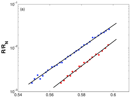
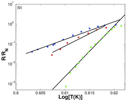
Figure 1: Data points obtained from Fig. 1 of Ref. [Giordano, ] presenting the resistance vs. $T$, re–plotted on a log–log scale; the solid lines correspond to fitting functions of the form $T^{\alpha}$. (a) In the low–$T$ (QPS) regime: blue circles (red squares) correspond to the samples of diameter $410\AA$ ($505\AA$); the corresponding exponents are $\alpha=25.2\pm 0.2$ and $\alpha=27.85\pm 0.4$, respectively. (b) The $410\AA$ and $505\AA$ diameter samples in the high–$T$ regime, and all data points of the $720\AA$ diameter sample (green diamonds); $\alpha=89\pm 13$, $\alpha=125\pm 8$ and $\alpha=260\pm 7$, respectively.

We first consider the data of Ref. [Giordano, ]. Fig. (1) presents the resistance of two samples as a function of $T$ on a log–log scale. Note that the length of the shortest wire studied is 80 $\mu$m. In comparison, the effective length set by the temperature scale $L_{T}=(v/T)$ for the relevant $T\sim 4\,K$ is of order 10 $\mu$m; this follows from the estimate $v\sim cd/\lambda_{L}$, where $c$ is the velocity of light and the measured $\lambda_{L}\approx 1300\AA$ obtained for Indium films of comparable thickness toxen . The wires therefore fulfill the long wire condition $L\gg L_{T}$, and can be considered good candidates for testing the scaling of $\rho(T)$ with $T$. In the low $T$ regime [Fig. (1(a))], the fit to a power–law is very goodrealTc . In addition, the values of $\alpha$ corresponding to the two samples of diameters $410\AA$ and $505\AA$ yield the Luttinger parameters $K=0.0735$ and $K=0.067$, respectively. These are consistent with the values obtained by inserting the relevant $d$ and $\lambda_{L}$ in Eq. (28), provided $C\approx 2$.

In principle, one may argue that a fit by a power–law with a high exponent (especially within a limited range of $T$) is not easily distinguishable from an exponential function. However, to put the above analysis to a further test, we tried to fit the data obtained in the high $T$ regime (in the close vicinity of $T_{c}$) to a power–law as well. In this regime, there is no justification for such a functional dependence on $T$, as the thermal activation theory for phase–slipsLAMH is expected to work much better. Indeed, the result depicted in Fig. (1(b)) indicates an obvious failure of a $T^{\alpha}$ trial function: the best fit to a straight line on a log–log plot yields an anomalously large exponent ($\alpha$ ranging from $89$ to $260$), and a systematic deviation from the fitting function. This is in sharp contrast with the situation in the low–$T$ regime, and therefore strengthen our confidence that in the latter case, the analysis is valid and provides a meaningful confirmation of the theoretical prediction.

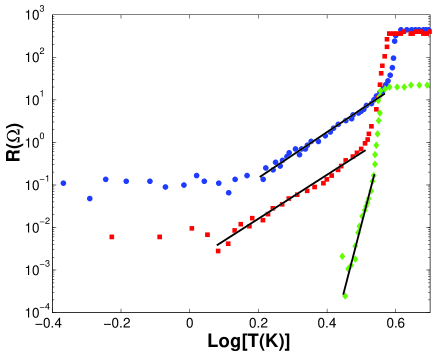
Figure 2: Data points obtained from Fig. 1 of Ref. [tian, ] presenting the resistance vs. $T$, re–plotted on a log–log scale: sample diameters are 20 nm (blue circles), 40 nm (red squares), and 60 nm (green diamonds). The solid lines correspond to fitting functions of the form $T^{\alpha}$, with $\alpha=5.38\pm 0.2$, $\alpha=5.16\pm 0.2$ and $\alpha=31.2\pm 1.3$, respectively.

We next consider the data of Tian et al (Ref. [tian, ]). The results obtained from resistivity measurements in three different tin (Sn) nanowires of diameters ranging between 20 nm and 60 nm are depicted in Fig. (2). Similarly to Giordano’s data, in all three samples a “kink” is observed at some temperature $T^{\ast}<T_{c}$, below which the decrease of $R$ as $T$ is lowered becomes more moderate. In the two thinner samples, the low–$T$ section of the data is quite noisy, and $R(T)$ seems to saturate. This behavior is possibly due to serial contribution from the contacts. Otherwise, however, the power–law dependence appears to be a good fit for $T<T^{\ast}$.

To test the validity of Eq. (28) in this system, one requires an independent estimate of $\lambda_{L}$. A direct measurement is not available, however, an indirect estimate of the ratio $\lambda_{L}/d$ based on a measurement of the effective critical magnetic fieldLiu yields $\lambda_{L}/d\approx 1.5$ for $d\approx 70$ nm, which is close in diameter to the thickest sample of Fig. (2). This is consistent with Eq. (28) for $C\approx 0.98$, a quite reasonable estimate for the capacitance. Unfortunately, reliable data on $\lambda_{L}/d$ in the thinner samples is not available. A naive extrapolation of the $d$–dependence of $\lambda_{L}$ to lower values of $d$ based on the Landau–Ginzburg theorySCbook ($\lambda_{L}\sim 1/\sqrt{d}$) yields $K=0.315$ for the $20$ nm sample, a reasonable approximation to the value of $K$ obtained from the fit ($K=0.274$), however the expected scaling with $d$ fails in the case of the $40$ nm sample. Indeed, as shown explicitly in Ref. [Liu, ], the naive scaling $\lambda_{L}(d)$ works well above $60$ nm, but breaks down for the $d=40$ nm wire (no data is given for even thinner samples).

We finally focus our attention on the most recent experimental work of Altomare et al. (Ref. [altomare, ]). This group has studied long and thin Aluminum wires, which appear to be ideal candidates for comparison with the QPS theory. In addition, the application of a magnetic field $H$ enables a continuous tuning of the superfluid density in a single sample of fixed $d$. Following Eq. (7), we therefore expect the $H$–dependence of $K$ to be related to $n_{s}$ via $1/K(H)\sim\sqrt{n_{s}(H)}$. The functional dependence of $n_{s}(H)$ on $H$ can be derived from a simple calculation using the Landau–Ginzburg theory at finite magnetic fieldSCbook . This yields

$$n_{s}(H)=n_{s}(0)\left(1-\frac{H^{2}}{H_{\parallel}^{2}}\right)\;,\quad H_{\parallel}\equiv\frac{\mathcal{N}\lambda_{L}}{d}H_{c}$$ (29)

where $H_{c}$ is the bulk critical field, and $\mathcal{N}$ a numerical factor which depends on the geometry: e.g., $\mathcal{N}=2\sqrt{6}$ in a thin film of thickness $d$, and $\mathcal{N}=8$ in a cylindrical wire of diameter $d$. $H_{\parallel}$ marks an estimated critical field where the inverse Luttinger parameter is expected to vanish according to

$$\frac{1}{K(H)}=\frac{1}{K(0)}\left(1-\frac{H^{2}}{H_{\parallel}^{2}}\right)^{1/2}\;.$$ (30)

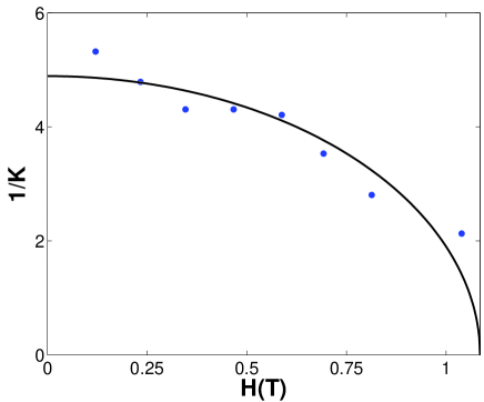
Figure 3: Data obtained from the unpublished notes (Ref. [altomare, ]), plotted in terms of the inverse Luttinger parameter ($1/K$) as a function of magnetic field $H$. All data points correspond to the lowest temperature measurements ($T=0.4$ K). The solid curve corresponds to the formula Eq. (30), with $H_{\parallel}\approx 1.1\,{\rm T}$.

The unpublished notes included in Ref. [altomare, ] enable a direct comparison of the experimental data to the above prediction. The experimental results include the Ohmic resistance as well as current–voltage characteristics which include a non–linear part. In the notes, it is shown that the latter can be fitted to a power–law $V\sim I^{\nu}$. This is suggested by the authors as a plausible alternative to the phenomenological exponential expression used as a fitting function in the published Letter. Such power–law in the $I-V$ characteristic is consistent with a $T$–dependence of the Ohmic resistance of the form $R(T)\sim T^{\alpha}$, with $\alpha=\nu-1$. The exponent $\nu$ is then extracted from the data for different values of the magnetic field, and plotted as a function of $H$. Using the linear relation of $\nu$ to $1/K$, we plot the data in the form depicted in Fig. (3), where it is fitted to a trial function of the form (30). The fit is reasonably successful, and is better than the $H$–dependence derived from Giordano’s formulaaltomare . It yields a critical field $H_{\parallel}\approx 1.1\,{\rm T}$.

To compare with an independent estimate of $H_{\parallel}$ based on the experimental parameters, we use the dirty limit expression for the bulk critical fieldSCbook $H_{c}=\phi_{0}/\pi 2^{2/3}\lambda_{L}\xi$ (with $\xi$ the SC coherence length in the dirty limit). Employing Eq. (29) we observe that, up to the numerical constant $\mathcal{N}$, $H_{\parallel}$ is essentially determined by $d$ and $\xi$ only. The experimental parameters mentioned in Ref. [altomare, ] imply $d\approx 60\AA$, $\xi\approx 1280\AA$ (the latter, however, relies on the text–book expression for $\xi$ in a dirty Aluminum and the measured mean free path). The wires are actually thin strips with a rectangular cross section, hence $\mathcal{N}$ cannot be determined accurately, but is expected to be intermediate between a thin film and a wire, yielding $H_{\parallel}$ between $1.4\,{\rm T}$ and $2\,{\rm T}$. The order of magnitude is consistent with the value extracted from Fig. (3). Considering the fact that the above estimate of $H_{\parallel}$ does not rely on any fitting parameters, this is a reasonably good agreement.

IV Conclusions

We have studied the low $T$ resistivity of a dirty SC wire using a memory formalism approach. This method allows a perturbative treatment of corrections to the low energy effective theory, describing the dynamics of phase fluctuations in the SC order parameter. In the limits of either ideally homogeneous wire or strongly inhomogeneous (granular) wire, our results for $\rho(T)$ recover the power–law behavior $\sim T^{\alpha}$ derived in earlier theoretical literature using the instanton technique. We show that more generally, the expression for $\rho(T)$ interpolates between the two limits, where the relative weights of each are smoothly tuned by a “granularity parameter” $D$ describing the typical fluctuations in the diameter of the wire. In particular, the inhomogeneity of the wire leads to an exponential enhancement of the phase–slips induced resistivity.

Following these calculations, we infer that the low energy theory is likely to be relevant to experimental measurements of $\rho(T)$ in the low $T$, QPS regime. We directly test the validity of the power–law ansatz as a fit to experimental data obtained in a variety of different samples, and found a very good agreement in sufficiently long wires. The exponent $\alpha$ extracted from the $\rho(T)$ data is found to be consistent with the values obtained from an independent estimate, based on known parameters of the corresponding samples (as much as the information was available). In addition, its dependence on a parallel magnetic field is consistent with the theoretical expectation. We conclude that the low–$T$ theory for dirty SC wires provides a plausible interpretation of data presented in the experimental literature, which is better justified than previously used phenomenological effective models. Our conclusions will hopefully encourage a further, more systematic investigation of the comparison between theory and experiment.

Appendix A Derivation of the Resistivity within the Memory Function Approach

In this Appendix we review the general aspects of the memory matrix approachforster ; woelfle ; giamarchi ; rosch , which turns out to serve as a useful tool for evaluating transport properties in systems where approximate conservation laws can be easily identified. As we show below, the calculation of d.c. electric resistivity of a SC wire provides a particularly simple example for the application of this approach, which amounts to a straightforward perturbative treatment of any processes responsible for relaxing the transport current.

At finite but low $T$, the fixed point Hamiltonian $H_{0}$ [Eq. (3)] provides the leading contribution to thermodynamic properties of the SC wire. However, by itself it does not give access to transport properties: being a translationally invariant integrable model, it possesses an infinite number of conserved currents, including in particular the electric charge transport current. Since the current cannot degrade, the d.c. conductivity is infinite even for $T>0$. To get the leading non–trivial contribution to transport, it is therefore necessary to add the irrelevant corrections, leading to a slow but finite relaxation rate of the currents. In our case, the prominent corrections are the phase–slips terms $H_{n}^{ps}$ [Eq. (4)]: note that other irrelevant terms, e.g., of the form $\int(\partial\phi)^{m}(\partial\theta)^{n}$, $\int(\partial^{m}\phi)(\partial\phi)^{n}$ with $n+m>2$ as well as pair breaking terms, which are already neglected in Eq. (2), do not contribute significantly to transportrosch ; SAR . We then evaluate the resistivity $\rho(T)$ employing the memory matrix approach, which takes advantage of the fact that the memory matrix – a matrix of decay–rates of the slowest modes in the system – is perturbative in the irrelevant operators. This is in contrast with the conductivity matrix, which is a highly singular function of these perturbations.

A crucial step in the derivation of transport coefficients in the memory matrix approach is the identification of primary slowly decaying currents of the system. These are conserved “charges” of the fixed point Hamiltonian $H_{0}$, whose conservation is slightly violated by certain irrelevant perturbations. In the case of the Luttinger model rosch , these include the charge current $J_{e}$ [Eq. (8)] and, in addition, the total translation operator

$$J_{T}=-\int dx\Pi\partial_{x}\phi\;.$$ (31)

In the above, we approximate the currents by contributions from the collective degrees of freedom (phase fluctuations) only. Non–superconducting contributions associated with unpaired electrons are exponentially suppressed as $e^{-\Delta/T}$ (with $\Delta\sim T_{c}$) for $T\ll T_{c}$. The correlators of $J_{e}$, $J_{T}$ determine the conductivity matrix $\hat{\sigma}(\omega,T)$ at frequency $\omega$ and temperature $T$ via the Kubo formula:

$$\sigma_{pq}(\omega,T)=\frac{1}{TL}\int_{0}^{\infty}dte^{i\omega t}\left(J_{p}(t)|J_{q}\right)\;,$$ (32)

where following Ref. [forster, ] we have introduced the scalar product (of any two operators $A$ and $B$)

$$\left(A(t)|B\right) \equiv T\int_{0}^{1/T}d\lambda\left\langle A(t)^{\dagger}B(i\lambda)\right\rangle\;.$$ (33)

The d.c. electrical resistivity is then given by $\rho(T)=1/\sigma_{ee}(T)$, where $\hat{\sigma}(T)$ is the $\omega\rightarrow 0$ limit of $\sigma_{ee}(\omega,T)$. However, a direct application of Eq. (32) at low $T,\omega$ is rather subtle: since $[J_{q},H_{0}]=0$ (for $q=e,T$), the relaxation rate of the currents $\partial_{t}J_{q}=i[J_{q},H]$ is dictated by the irrelevant corrections, hence tends to vanish in the limit $T\rightarrow 0$. This leads to divergences in the conductivities, since the currents do not decay in this limit.

To enable a controlled perturbative expansion in the relaxation rates $\partial_{t}J_{q}$, we therefore recast the conductivity matrix in terms of a memory matrix $\hat{M}$:

$$\hat{\sigma}(\omega,T) = \hat{\chi}(T)\left(\hat{M}(\omega,T)-i\omega\hat{\chi}(T)\right)^{-1}\hat{\chi}(T),$$ (34)

in which

$${M}_{pq}(\omega,T)\equiv\frac{1}{TL}\left(\partial_{t}J_{p}\left|{\mathcal{Q}}\frac{i}{\omega-{\mathcal{Q}}{\mathcal{L}}{\mathcal{Q}}}{\mathcal{Q}}\right|\partial_{t}J_{q}\right)$$ (35)

and $\hat{\chi}$ is the matrix of static susceptibilities

$${\chi}_{pq}=\frac{1}{TL}(J_{p}|J_{q})\;.$$ (36)

Here ${\mathcal{L}}$ is the Liouville operator defined by ${\mathcal{L}}A=[H,A]$, and ${\mathcal{Q}}$ is the projection operator on the space perpendicular to the slowly varying variables $J_{q}$,

$${\mathcal{Q}}=1-\sum_{pq}|J_{p})\frac{1}{TL}(\hat{\chi}^{-1})_{pq}(J_{q}|\;.$$ (37)

Note that similarly to Ref. [SAR, ], we choose a convenient definition of the memory matrix [Eq. (35)], which is slightly different than the standard literature. The perturbative nature of $\hat{M}$ is transparently reflected by this expression: in particular, the operators $\partial_{t}J_{q}$ are already linear in the irrelevant corrections to $H_{0}$. This enables a systematic perturbative expansion of the correlator in Eq. (35) in the small parameter characterizing the relative size of the corrections – in our case, the exponential factors $y^{n}$ [see Eq. (4)].

We now obtain an expression for the d.c. electric resistivity by setting $\omega=0$ in Eq. (34). This yields

$$\rho(T)=\frac{M_{ee}M_{TT}-M_{eT}^{2}}{\chi_{ee}^{2}M_{TT}+2\chi_{eT}\chi_{ee}M_{eT}+\chi_{eT}^{2}M_{ee}}\,,$$ (38)

where $\hat{M}$ is evaluated from Eq. (35) in the limit $\omega\rightarrow 0$. (Note that here we have used the fact that both matrices $\hat{M}(T)$ and $\hat{\chi}(T)$ are symmetric.) The relaxation rate operators $\partial_{t}J_{q}$ are given by

$$\partial_{t}J_{q}=\sum_{n}F_{ps,n}^{q}\;,$$ (39)

where we have defined the ‘force’ operators

$$F_{ps,n}^{q}\equiv i[J_{q},H_{n}^{ps}]\;.$$ (40)

To leading order in the perturbations $H_{n}^{ps}$, Eq. (35) for $\hat{M}$ is greatly simplified: one can set ${\mathcal{L}}={\mathcal{L}}_{0}$ with ${\mathcal{L}}_{0}=[H_{0},.]$ and ${\mathcal{Q}}=1$. This yields

$$\hat{M}(T)\approx\sum_{n}\hat{M}_{ps,n}\;,$$ (41)

where the elements of $\hat{M}_{ps,n}$ are given by

$$M_{ps,n}^{pq}\equiv\lim_{\omega\rightarrow 0}\frac{\langle F_{ps,n}^{p};F_{ps,n}^{q}\rangle^{0}_{\omega}-\langle F_{ps,n}^{p};F_{ps,n}^{q}\rangle^{0}_{\omega=0}}{i\omega}$$ (42)

in which $\langle F^{p};F^{q}\rangle^{0}_{\omega}$ is the retarded correlation function evaluated with respect to $H_{0}$.

Substituting Eqs. (31) and (4) in Eq. (40) and taking the $L\rightarrow\infty$ limit, it is easy to see that $F_{ps,n}^{T}=0$. Indeed, this follows from the translational invariance of $H_{n}^{ps}$. As a result, $M_{TT}$ and $M_{eT}$ identically vanish. This implies that if both $\chi_{eT}$ and $M_{ee}$ do not vanish, Eq. (38) yields $\rho(T)=0$ even at finite $T$; namely, the creation of free phase–slips appears to be insufficient to generate a finite dissipation. Such a result cannot be reconciled with our understanding, that dissipation should occur at the normal cores during a phase–slips event, where the wire behaves temporarily as a normal dirty metal. Indeed, we should recall that the translational invariance of $H_{n}^{ps}$ is not of microscopic origin; rather, these terms in the effective Hamiltonian are obtained after averaging over disorder in the electron systemzaikin_prb . Their form reflects the total absorption of the finite momentum $P=2\pi sn_{s}$ generated in a phase–slip process by the core electrons. In a clean SC wire, such momentum transfer is not effective, leading to an exponential suppression of $M_{TT}$, $M_{ee}$ and yielding a finite but exponentially small resistivity $\rho(T)\sim e^{-vP/2T}$ (see Ref.  [khleb1, ; KP, ]). Stronger disorder in the underlying electronic system should only enhance the resistivity, and not vice versa! This apparent paradox is resolved by the remarkable observationRA_JLTP that, following the commensurate relation between the total momentum $P$ and density per unit length, $\chi_{eT}$ actually vanishes identically, even at finite $T$. Setting $\chi_{eT}=0$ in Eq. (38), we then find that the expression for the resistivity $\rho(T)$ reduces to the simplified form Eq. (9).

The above arguments are accurate as long as indeed the currents $J_{e}$, $J_{T}$ are given by Eqs. (8), (31), i.e., when normal electron contributions to the currents are neglected. However, if such normal contributions are not negligible, they would at the same time modify the translation invariance of the Hamiltonian, and all entries in Eq. (38) would be finite. Similarly, translational invariance is explicitly broken once we account for random spatial fluctuations in the SC wire cross section, by introducing the inhomogeneous phase–slip term Eq. (21). This modifies the force operator $F_{ps}^{e}$ [now given by Eq. (24)], and induces a non–trivial contribution to $F_{ps}^{T}$:

$$F_{ps}^{T}=-i\frac{2}{\pi}\>v^{2}\int dx\>y(x)\>\left(\partial_{x}\theta\right)\>\sin\left(2\theta\right)\;.$$

However, the resulting matrix $\hat{M}(T)$ obtained after substitution in the approximate form Eq. (42) is still diagonal: to see this, we note that the off-diagonal element is given (after disorder averaging) by

$$M_{eT} \approx\frac{4evLy_{0}^{2}}{K}$$

$$\times \int_{0}^{\infty}dt\,t\,\int_{-\infty}^{\infty}dx\;\overline{e^{-\Lambda(x)}e^{-\Lambda(0)}}\;{\rm Im}\{C_{eT}(x,t)\}$$

where

$$C_{eT}(x,t) = 2\partial_{x}G_{\theta}(x,t)e^{4G_{\theta}(x,t)}\;,$$ (44)

in which $G_{\theta}(x,t)$ is given by Eq. (18). It is apparent from Eqs. (44) and (18) that $C_{eT}(x,t)$ is an antisymmetric function of $x$, and hence the integral over $x$ in Eq. (A) vanishes, yielding $M_{eT}=0$. The static susceptibility matrix [Eq. (36)] evaluated to leading order in the perturbation $H_{sp}$ is also approximately diagonal, with $\chi_{ee}$ given by Eq. (14). We therefore find that the leading contribution to Eq. (38) for the resistivity again practically reduces to Eq. (9).

References

- (1) W. A. Little, Phys. Rev. 156, 396 (1967).
- (2) J. S. Langer and V. Ambegaokar, Phys. Rev. 164, 498 (1967); D. E. McCumber and B. I. Halperin, Phys. Rev. B 1, 1054 (1970).
- (3) See, e.g., R. S. Newbower, M. R. Beasley and M. Tinkham, Phys. Rev. B 5, 864 (1972).
- (4) N. Giordano, Phys. Rev. Lett. 61, 2137 (1988); N. Giordano, Phys. Rev. B 41, 6350 (1990).
- (5) A. O. Caldeira and A. J. Leggett, Phys. Rev. Lett. 46, 211 (1981); A. O. Caldeira and A. J. Leggett, Ann. of Phys. 149, 347 (1983).
- (6) J. -M. Duan, Phys. Rev. Lett. 74, 5128 (1995).
- (7) S. R. Renn and J. -M. Duan, Phys. Rev. Lett. 76, 3400 (1996).
- (8) A. D. Zaikin, D. S. Golubev, A. van Otterlo and G. T. Zimanyi, Phys. Rev. Lett. 78, 1552 (1997).
- (9) A. van Otterlo, D. S. Golubev, A. D. Zaikin and G. Blatter, Eur. Phys. J. B 10, 131 (1999); D. S. Golubev and A. D. Zaikin, Phys. Rev. B 64, 014504 (2001).
- (10) S. Khlebnikov, Phys. Rev. Lett. 93, 090403 (2004).
- (11) S. Khlebnikov and L. P. Pryadko, Phys. Rev. Lett. 95, 107007 (2005).
- (12) G. Refael, E. Demler, Y. Oreg and D. S. Fisher, Phys. Rev. B 75, 014522 (2007).
- (13) J. M. Kosterlitz and D. J. Thouless, J. Phys. C 6, 1181 (1973); J. M. Kosterlitz, J. Phys. C 7, 1046 (1974).
- (14) J. -M. Duan, Phys. Rev. Lett. 79, 3316 (1997).
- (15) A. Bezryadin, C. N. Lau, and M. Tinkham, Nature 404, 971 (2000).
- (16) C. N. Lau, N. Markovic, M. Bockrath, A. Bezryadin and M. Tinkham, Phys. Rev. Lett. 87, 217003 (2001).
- (17) M. Tian, J. Wang, J. S. Kurtz, Y. Liu, M. H. W. Chan, T. S. Mayer, and T. E. Mallouk, Phys. Rev. B 71, 104521 (2005).
- (18) M. Zgirski, K -P Riikonen, V. Touboltsev, and K. Arutyunov, Nano Lett. 5, 1029 (2005).
- (19) F. Altomare, A. M. Chang, M. R. Melloch, Y. Hong, and C. W. Tu, Phys. Rev. Lett. 97, 017001 (2006); see also unpublished notes, cond-mat/0505772.
- (20) K. Arutyunov et al., unpublished.
- (21) See, e.g., Chapter 9 in P. M. Chaikin and T. C. Lubensky, Principles of Condensed Matter Physics (Cambridge University Press, 1995).
- (22) J. E. Mooij and G. Schön, Phys. Rev. Lett. 55, 114 (1985).
- (23) D. Forster, Hydrodynamic Fluctuations, Broken Symmetry, and Correlation Functions, (Benjamin, Massachusetts, 1975).
- (24) W. Götze and P. Wölfle, Phys. Rev. B 6, 1226 (1972).
- (25) T. Giamarchi, Phys. Rev. B 44, 2905 (1991).
- (26) A. Rosch and N. Andrei, Phys. Rev. Lett. 85, 1092 (2000).
- (27) P. Jung and A. Rosch, Phys. Rev. B 75, 245104 (2007).
- (28) See, e.g., H. J. Schultz, Phys. Rev. B 34, 6372 (1986).
- (29) T. Giamarchi, Quantum Physics in One Dimension (Oxford University Press, 2004).
- (30) T. Giamarchi and H. J. Schultz, Phys. Rev. B 37, 325 (1988).
- (31) D. Meidan, Y. Oreg and G. Refael, Phys. Rev. Lett. 98, 187001 (2007).
- (32) A. M. Toxen, Phys. Rev. 123, 442 (1961).
- (33) It should be pointed out that the crossover temperature is not too far from the value of as quoted by Giordano in Ref. [Giordano, ], which corresponds to the thin film critical temperature, assumed to apply for the wire as well. As a consequence, one might expect a –dependence of the exponent associated mainly with the –dependence of near . Such deviation from a pure power–law is, however, not supported by the experimental data for . A possible resolution for that might be that the actual in a wire and film are actually quite different. Indeed, depends crucially on dimensionality: for example, it is significantly enhanced in a thin film compared to the bulk (three–dimensional) material. In practice, is often treated as a fitting parameter (see, e.g., Ref. [oreg, ]).
- (34) Y. Liu, private communication.
- (35) M. Tinkham, Introduction to Superconductivity (McGraw–Hill Inc., 1975).
- (36) E. Shimshoni, N. Andrei and A. Rosch, Phys. Rev. B 68, 104401 (2003).
- (37) A. Rosch and N. Andrei, J. of Low Temp. Phys. 126, 1195 (2002).