Quantum CISC Compilation by Optimal Control and
Scalable Assembly of Complex Instruction Sets beyond Two-Qubit Gates

Zusammenfassung

We present a quantum cisc compiler and show how to assemble complex instruction sets in a scalable way. Enlarging the toolbox of universal gates by optimised complex multi-qubit instruction sets thus paves the way to fight relaxation for realistic experimental settings.

Compiling a quantum module into the machine code for steering a concrete quantum hardware device lends itself to be tackled by means of optimal quantum control. To this end, there are two opposite approaches: (i) one may use a decomposition into the restricted instruction set (risc) of universal one- and two-qubit gates and translate them into the machine code, or (ii) one may prefer to generate the entire target module as a complex instruction set (cisc) directly by evoltution under drift and available controls. Here we advocate direct compilation up to the limit of system size a classical high-performance parallel computer cluster can reasonably handle. For going beyond these limits, i.e. for large systems, we propose a combined way, namely (iii) to make recursive use of medium-sized building blocks generated by optimal control in the sense of a quantum cisc compiler.

The advantage of the method over standard risc compilations into one- and two-qubit universal gates is explored on the parallel cluster hlrb-ii (with a total linpack performance of $63.3$ TFlops/s) for the quantum Fourier transform, the indirect swap gate as well as for multiply-controlled not gates. Implications for upper limits to time complexities are also derived.

Introduction

Richard Feynman’s seminal conjecture of using experimentally controllable quantum systems to perform computational tasks Feynman (1982, 1996) roots in reducing the complexity of the problem when moving from a classical setting to a quantum setting. The most prominent pioneering example being Shor’s quantum algorithm of prime factorisation Shor (1994, 1997) which is of polynomial complexity (bqp) on quantum devices instead of showing non-polynomial complexity on classical ones Papadimitriou (1995). It is an example of a class of quantum algorithms Jozsa (1998); Cleve et al. (1998) that solve hidden subgroup problems in an efficient way Ettinger et al. (2004), where in the Abelian case, the speed-up hinges on the quantum Fourier transform (qft). Whereas the network complexity of the fast Fourier transform (fft) for $n$ classical bits is of order $O(n2^{n})$ Cooley and Tukey (1965); Beth (1984), the qft for $n$ qubits shows a complexity of order $O(n^{2})$. Moreover, Feynman’s second observation that quantum systems may be used to efficiently predict the behaviour of other quantum systems has inaugurated a branch of research dedicated to Hamiltonian simulation Lloyd (1996); Abrams and Lloyd (1997); Zalka (1998); Bennett et al. (2002); Masanes et al. (2002); Jané et al. (2003).

For implementing a quantum algorithm in an experimental setup, local operations and universal two-qubit quantum gates are required as a minimal set ensuring every unitary module can be realised Deutsch (1985). More recently, it turned out that generic qubit and qudit pair interaction Hamiltonians suffice to complement local actions to universal controls Dodd et al. (2002); Bremner et al. (2005). Common sets of quantum computational instructions comprise (i) local operations such as the Hadamard gate, the phase gate and (ii) the entangling operations cnot, controlled-phase gates, $\sqrt{\text{\sc swap}}$, $i$ swap as well as (iii) the swap operation. The number of elementary gates required for implementing a quantum module then gives the network or gate complexity.

As is well known, a generic $n$-qubit generic operation requires exponentially many two-qubit gates to be implemented exactly Barenco et al. (1995); Knill (1995), the complexity being $O(n4^{n})$. Yet, as has been pointed out by Barenco et al., many quantum computationally pertinent gates can be decomposed into a number of one- and two-qubit gates increasing linearly with the number of qubits. At the expense of a single ancilla qubit this also holds for multiply controlled unitary gates Barenco et al. (1995) tantamount to error correction. For an overview, see e.g. Nielsen and Chuang (2000); Kitaev et al. (2002); Mermin (2007). Moreover, Blais Blais (2001) showed how to implement the QFT with linear gate complexity. Later, Solovay (Solovay (1995) quoted in Kitaev (1997) and Nielsen and Chuang (2000)) and then Kitaev addressed the problem to approximate arbitrary unitary gates by polynomially long 2-qubit gate sequences up to a given precision Kitaev (1997); Kitaev et al. (2002). More recently the bounds of approximating an arbitrary unitary were taken down to a polynomial of sixth-order in the number of qubits and of third order in the geodesic distance of the unitray to unity Nielsen et al. (2006). Differential geometric aspects in terms of Finsler metrics have been raised in Nielsen (2006).

$$\mathrm{Program},\mathrm{Module}$$    $$\mathrm{Quantum}\mathrm{Algorithm},\mathrm{Unitary}\mathrm{Module}$$

$$\setcounter{MaxMatrixCols}{11}\begin{CD}@V{{\rm Compiler}}V{{\rm(RISC\;or\;CISC)}}V@V{}V{}V@V{{\rm{RISC}-Compiler}}V{\rm\bf(1)}V@V{}V{\rm\bf(2)}V@V{\rm{CISC}-Compiler}V{\rm\bf(3)}V\hskip 5.69054pt\\ \boxed{\;\text{Assembler\phantom{$(^{!}$}Code}\;}&&\hskip 22.76219pt\text{\quad\/``direct\/''}\hskip 25.60747pt\boxed{\;\text{Universal\phantom{$(^{!}$}Gates\;\;({\sc risc})}\;}&&\text{\quad\; {single {\sc cisc} \quad\;}}&&\boxed{\text{\; {Optimal\phantom{$(^{!}$}Controls\; ({\sc cisc})\;}}}\\ @V{\rm Assembler}V{}V@V{}V{}V@V{\rm Assembler}V{}V@V{}V{}V@V{\rm scalable\;Assembler}V{}V\hskip 5.69054pt\\ \end{CD}\vspace{-2mm}$$

$$\mathrm{Machine}\mathrm{Code}$$    $$\mathrm{Machine}\mathrm{Code}\mathrm{of}\mathrm{Quantum}\mathrm{Evolutions}\mathrm{under}\mathrm{Drift}\mathrm{and}\mathrm{Controls}$$

Abbildung 1: Compilation in classical computation (left) and quantum computation (right). Quantum machine code has to be time-optimal or protected against relaxation, otherwise the coherent superpositions are wiped out. A quantum risc-compiler (1) by universal gates leads to unnecessarily long machine code. Direct cisc-compilation into a single pulse sequence (2) exploits quantum control for a near time-optimal quantum machine code. Its classical complexity is np, so direct compilation by numerical optimal control resorting to a classical computer is unfeasible for large quantum systems. The third way (3) promoted here pushes quantum cisc-compilation to the limits of classical supercomputer clusters and then assembles the multi-qubit complex instructions sets recursively into time-optimised or relaxation-protected quantum machine code.

However, gate complexity often translates into too coarse an estimate for the actual time required to implement a quantum module (see e.g. Vidal et al. (2002); Childs et al. (2003); Zeier et al. (2004)), in particular, if the time scales of a specific experimental setting have to be matched. Instead, effort has been taken to give upper bounds on the actual time complexity Wocjan et al. (2002), e.g., by way of numerical optimal control Schulte-Herbrüggen et al. (2005).

Interestingly, in terms of quantum control theory, the existence of universal gates is equivalent to the statement that the quantum system is fully controllable as has first been pointed out in Ref. Ramakrishna and Rabitz (1995). This is, e.g., the case in systems of $n$ spin-$\tfrac{1}{2}$ qubits that form Ising-type weak-coupling topologies described by arbitrary connected graphs Schulte-Herbrüggen (1998); Glaser et al. (1998). Therefore the usual approach to quantum compilation in terms of local plus universal two-qubit operations Tucci (1999); Williams (2004); Shende et al. (2006); Svore et al. (2006); Tucci (2007) lends itself to be complemented by optimal-control based direct compilation into machine code: it may be seen as a technology-dependent optimiser in the sense of Ref. Svore et al. (2006), however, tailored to deal with more complex instruction sets than the usual local plus two-qubit building blocks. Not only is it adapted to the specific experimental setting, it also allows for fighting relaxation by either being near timeoptimal or by exploiting relaxation-protected subspaces Schulte-Herbrüggen et al. (2006). Devising quantum compilation methods for optimised realisations of given quantum algorithms by admissible controls is therefore an issue of considerable practical interest. Here it is the goal to show how quantum compilation can favourably be accomplished by optimal control: the building blocks for gate synthesis will be extended from the usual set of restricted local plus universal two-qubit gates to a larger toolbox of scalable multi-qubit gates tailored to yield high fidelity in short time given concrete experimental settings.

Quantum Compilation as an Optimal Control Task

As shown in Fig. 1, the quantum compilation task can be addressed following different principle guidelines: (1) by the standard decomposition into local operations and universal two-qubit gates, which by analogy to classical computation was termed reduced instruction set quantum computation (risc) Sanders et al. (1999) or (2) by using direct compilation into one single complex instruction set (cisc) Sanders et al. (1999). The existence of a such a single effective gate is guaranteed simply by the unitaries forming a group: a sequence of local plus universal gates is a product of unitaries and thus a single unitary itself.

As a consequence, cisc quantum compilation lends itself for resorting to numerical optimal control (on clusters of classical computers) for translating the unitary target module directly into the ‘machine code’ of evolutions of the quantum system under combinations of the drift Hamiltonian $H_{0}$ and experimentally available controls $H_{j}$.

In a number of studies on quantum systems up to 10 qubits, we have shown that direct compilation by gradient-assisted optimal control Khaneja et al. (2005); Schulte-Herbrüggen et al. (2005); Spörl et al. (2007) allows for substantial speed-ups, e.g., by a factor of $5$ for a cnot and a factor of $13$ for a Toffoli-gate on coupled Josephson qubits Spörl et al. (2007). However, the direct approach naturally faces the limits of computing quantum systems on classical devices: upon parallelising our C++ code for high-performance clusters Gradl et al. (2006), we found that extending the quantum system by one qubit increases the cpu-time required for direct compilation into the quantum machine code of controls by roughly a factor of eight. So the classical complexity for optimal-control based quantum compilation is np.

Therefore, here we advocate a third approach (3) that uses direct compilation into multi-qubit complex instruction sets up to the cpu-time limits of optimal quantum control on classical computers: these building blocks are designed such as to allow for recursive scalable quantum compilation in large quantum systems (i.e. those beyond classical computability). In particular, the complex instruction sets may be optimised such as to fight relaxation by being near time-optimal, or, moreover, they may be devised such as to fight the specific imperfections of an experimental setting.

Controllability

Before turning to optimal-control based cisc quantum compilation in more detail, it is important to ensure the quantum control system characterised by $\{H_{0}\}\cup\{H_{j}\}$ is in fact fully controllable.

Hamiltonian quantum dynamics following Schrödinger’s equation for the unitary image of a complete basis set of ‘state vectors’ representing a quantum gate

$$|\dot{\psi}(t)\rangle{} = -i\big{(}H_{d}+\sum_{j=1}^{m}u_{j}(t)H_{j}\big{)}\;|\psi(t)\rangle{}$$ (1)

$${\dot{U}(t)} = -i\big{(}H_{d}+\sum_{j=1}^{m}u_{j}(t)H_{j}\big{)}\;{U(t)}\quad,$$ (2)

resembles the setting of a standard bilinear control system with state $X(t)$, drift $A$, controls $B_{j}$, and control amplitudes $u_{j}\in\mathbb{R}^{\,}{}$ reading

$$\dot{X}(t)=\big{(}A+\sum_{j=1}^{m}u_{j}(t)B_{j}\big{)}\;X(t)\quad,$$ (3)

where $X(t)\in{GL}_{N}(\mathbb{C}^{\,}{})$ and $A,B_{j}\in\operatorname{Mat}{}_{N}(\mathbb{C}^{\,}{})$. Clearly in the dynamics of closed quantum systems, the system Hamiltonian $H_{d}$ is the drift term, whereas the $H_{j}$ are the control Hamiltonians with $u_{j}(t)$ as control amplitudes. In systems of $n$ qubits, $|\psi\rangle{}\in\mathbb{C}^{\,2^{n}}{}$, $U\in SU(2^{n})$, and $i\,H_{\nu}\in\mathfrak{su}(2^{n})$.

A system is fully operator controllable, if to every initial state $\rho_{0}$ the entire unitary orbit $\mathcal{O}_{\rm U}(\rho_{0}):=\{U\rho_{0}U^{\dagger}\;|\;U\in SU(N)\}$ can be reached. With density operators being Hermitian this means any final state $\rho(t)$ can be reached from any initial state $\rho_{0}$ as long as both of them share the same spectrum of eigenvalues.

As established in Jurdjevic and Sussmann (1972), the bilinear system of Eqn. 2 is fully controllable if and only if the drift and controls are a generating set of $\mathfrak{su}(N)$ by way of the commutator, i.e., $\langle{H_{d},H_{j}}\,|\,j=1,2,\dots,m\rangle_{\rm Lie}={\mathfrak{su}(N)}$.

Example 1 Consider a system of $n$ weakly coupled spin-$\tfrac{1}{2}$ qubits. Let $\sigma_{x}=\left(\begin{smallmatrix}\,0&\,1\,\\ \,1&\,0\,\end{smallmatrix}\right)$, $\sigma_{y}=\left(\begin{smallmatrix}0&-i\\ i&\phantom{-}0\end{smallmatrix}\right)$, $\sigma_{z}=\left(\begin{smallmatrix}1&\phantom{-}0\\ 0&-1\end{smallmatrix}\right)$ be the Pauli matrices. In $n$ spins-$\tfrac{1}{2}$, a $\sigma_{kx}$ for spin $k$ is tacitly embedded as ${\rm 1\negthickspace l}{}\otimes\cdots{\rm 1\negthickspace l}{}\otimes\sigma_{x}\otimes{\rm 1\negthickspace l}{}\otimes\cdots{\rm 1\negthickspace l}{}$ where $\sigma_{x}$ is at position $k$. The same holds for $\sigma_{ky}$, $\sigma_{kz}$, and in the weak coupling terms $\sigma_{kz}\sigma_{\ell z}$ with $1\leq k<\ell\leq n$.

Now a system of $n$ qubits is fully controllable Schulte-Herbrüggen (1998), if e.g. the control Hamiltonians $H_{j}$ comprise the Pauli matrices $\{{\sigma_{kx},\sigma_{ky}}\,|\,k=1,2,\dots n\}$ on every single qubit selectively and the drift Hamiltonian $H_{d}$ encompasses the Ising pair interactions $\{{J_{k\ell}}\;{(\sigma_{kz}\sigma_{\ell z})/2}\,|\,k<\ell=2,\dots n\}$, where the coupling topology of $J_{k\ell}\neq 0$ may take the form of any connected graph. This theorem has meanwhile been generalised to other coupling types Schulte-Herbrüggen et al. (2002); Albertini and D’Alessandro (2002).

In view of the compilation task in quantum computation we get the following synopsis:

Corollary 1

The following are equivalent:

1. in a quantum system of $n$ coupled spins-$\tfrac{1}{2}$, the drift $H_{d}$ and the controls $H_{j}$ form a generating set of $\mathfrak{su}(2^{n})$;

2. the quantum system is operator controllable (in the sense of Ref. Albertini and D’Alessandro (2003));

3. every unitary transformation $U\in SU(2^{n})$ can be realised by that system;

4. there is a set of universal quantum gates for the quantum system.

Proof: The equivalence of (1) and (2) relies on the unitary group being a compact connected Lie group: compact connected Lie groups have no closed subsemigroups that are no groups themselves Jurdjevic and Sussmann (1972). Moreover, in compact connected Lie groups the exponential mapping is surjective, hence (1) $\Rightarrow$ (3). Assertions (3) and (4) just re-express the same fact in different terminology. $\hfill\blacksquare$

Scope and Organisation of the Paper

The purpose of this paper is to show that optimal control theory can be put to good use for devising multi-qubit building blocks designed for scalable quantum computing in realistic settings. Note these building blocks are no longer meant to be universal in the practical sense that any arbitrary quantum module should be built from them (plus local controls). Rather they provide specialised sets of complex instructions tailored for breaking down typical tasks in quantum computation with substantial speed gains compared to the standard compilation by decomposition into one-qubit and two-qubit gates. Thus a cisc quantum compiler translates into significant progress in fighting relaxation.

For demonstrating quantum cisc compilation and scalable assembly, in this paper we choose systems with linear coupling topology, i.e., qubit chains coupled by nearest-neighbour Ising interactions. The paper is organised as follows: cisc quantum compilation by optimal control will be illustrated in three different, yet typical examples

1. the indirect $1,n$-swap gate,

2. the quantum Fourier transform (qft) ,

3. the generalisation of the cnot and Toffoli gate to multiply-controlled not gates, cⁿnot.

For every instance of $n$-qubit systems, we analyse the effects of (i) sacrificing universality by going to special instruction sets tailored to the problem, (ii) extending pair interaction gates to effective multi-qubit interaction gates, and (iii) we compare the time gain by recursive $m$-qubit cisc-compilation ($m\leq n$) to the two limiting cases of the standard risc-approach ($m=2$) on one hand and the (extrapolated) time-complexity inferred from single-cisc compliation (with $m=n$).

Preliminaries

Time Standards

When comparing times to implement unitary target gates by the risc vs the cisc approach, we will assume for simplicity that local unitary operations are ‘infinitely’ fast compared to the duration of the Ising coupling evolution so that the total gate time is solely determined by the coupling evolutions unless stated otherwise. Let us emphasise, however, this stipulation only concerns the time standards. The optimal-control assisted cisc-compilation methods presented here are in no way limited to fast local controls. In particular, also the assembler step of concatenating the cisc-building blocks is independent of the ratio of times for local operations vs coupling interactions.

Overview on Gate and Time Complexities

For practical purposes, the complexity of a unitary quantum operation can be expressed in terms of two measures: the gate complexity counts the number of universal one- and two-qubit gates for exactly implementing the target operation in a circuit. Moreover, in view of fighting relaxation, we will estimate the time complexity in terms of consecutive time-slots with simultaneous $m$-qubit modules required.

In order not to raise false expectations, upon changing from universal 2-qubit decompositions (risc) to $m$-qubit cisc-implementations the gate complexity for exact implemention of a generic $n$-qubit unitary operation clearly remains np: it requires ‘exponentially many’ $2$-qubit modules or $m$-qubit modules ($m\geq 2$) alike, yet a cut from the order of roughly $4^{n}/4^{2}$ necessary $2$-qubit modules down to some $4^{n}/4^{m}$ $m$-qubit modules (with up to $m=10$) is substantial and particularly valuable in few-qubit systems. More elaborate estimates will be given shortly. — Likewise, also in target modules with linear 2-qubit risc complexity, $m$-qubit cisc complexity remains linear, yet when translated into time complexity it may entail sizeable speed-ups – we will show examples where they allow for accelerations by more than a factor of $13$.

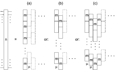
Abbildung 2: Decomposition of an $n$-qubit gate into a circuit of $m$-qubit gates, where $m$ is a uniform block size and may consist of risc modules $m=2$ or cisc modules with $m>2$. (a) Margolus pattern with $\tfrac{n}{m}$ integer, (b) $n-m\lfloor\tfrac{n}{m}\rfloor{}=\mu$ or (c) $n-m\lfloor\tfrac{n}{m}\rfloor{}=2\mu$, so $\mu>0$ integer.

To be more precise, a lower bound for the number of two-qubit gates necessary to exactly implement a a generic $n$-qubit unitary target module was given by Barenco et al. Barenco et al. (1995). Their parameter-counting argument is based on a gem, which deserves to be picked up for generalising it to realisations by $m$-qubit modules as illustrated in Fig. 2. The key is that only in the first time slot the number of parameters directly relates to the unitary group, while from the second slot onwards the parameters have to be counted in terms of cosets of the form $SU(2^{m})/(SU(2^{m-\mu})\otimes SU(2^{\mu}))$, if the $m$-qubit module has overlaps of $\mu$ qubits and $(m-\mu)$ qubits with the two adjacent modules in the time slot before. The number of real parameters (denoted by $\#$ for short) in the respective basic building bocks amount to

$$\#SU(2^{m}) = 4^{m}-1$$ (4)

$$\#\frac{SU(2^{m})}{SU(2^{m-\mu})\otimes{\rm 1\negthickspace l}{}_{2^{\mu}}} = 4^{m}-1-(4^{m-\mu}-1)$$ (5)

$$= 4^{m-\mu}(4^{\mu}-1)\quad$$

$$\#\frac{SU(2^{m})}{SU(2^{m-\mu})\otimes SU(2^{\mu})} = 4^{m}-1-(4^{m-\mu}-1)-(4^{\mu}-1)$$ (6)

$$= (4^{m-\mu}-1)(4^{\mu}-1)\quad.$$

Tabelle 1: Lower Bounds to Gate Complexities and Time Complexities for Implementing Generic $n$-Qubit Unitaries $SU(2^{n})$

$n$-qubit operation with $n=$	$2$	$3$	$4$	$5$	$6$	$7$	$8$	$9$	$10$	$20$	$100$
no of 2-qubit gates ($g_{2}$)	$1$	$6$	$27$	$112$	$453$	$1,818$	$7,279$	$29,124$	$116,505$	$1.22\times 10^{11}$	$1.79\times 10^{59}$
no of 2-qubit time slots ($t_{2}$)	$1$	$6$	$14$	$56$	$151$	$606$	$1,820$	$7,281$	$23,301$	$1.22\times 10^{10}$	$3.57\times 10^{57}$
no of 10-qubit gates ($g_{10}$)									$1$	$1,050,627$	$1.54\times 10^{54}$
no of 10-qubit time slots ($t_{10}$)									$1$	$525,314$	$1.54\times 10^{53}$

With these stipulations one may readily determine the number of $m$-qubit gates in a unitary network of the type of Fig. 2 a, where ${\frac{n}{m}}$ is integer, such as to ensure to exhaust the number $4^{n}-1$ of parameters of a generic $n$-qubit target gate to be implemented. In the first time slot there are ${\frac{n}{m}}$ parallel $m$-qubit gates (counting by the number of parameters in the group according to Eqn.4), in the second time slot there are $({\frac{n}{m}}-1)$ parallel $m$-qubit gates. They contribute the number of parameters of the coset (Eqn. 6), where one is forced to choose $\mu=\tfrac{m}{2}$ for even $m$ and $\mu=\tfrac{1}{2}(m\pm 1)$ for odd $m$ in order to be efficient. Following the same Margolus pattern one adds as many $m$-qubit gates (counting cosets) as required to superseed $4^{n}-1$ parameters. Using Gauss’ brackets one thus obtains the number $g_{m}$ of $m$-qubit gates needed to implement a generic $n$-qubit target gate

$$g_{m}=\Big{\lceil}\;{\frac{4^{n}-1-{\frac{n}{m}}(4^{m}-1)}{4^{m}-4^{\mu}-4^{m-\mu}+1}+{\frac{n}{m}}}\;\Big{\rceil}$$ (7)

and the respective number of time slots $t_{m}=\lceil\tfrac{g_{m}}{\lfloor\frac{n}{m}\rfloor{}}\rceil{}$ by

$$t_{m}=1+\Big{\lceil}\;{\frac{4^{n}-1-{\frac{n}{m}}(4^{m}-1)}{{\frac{n}{m}}(4^{m}-4^{\mu}-4^{m-\mu}+1)}}\;\Big{\rceil}\quad.$$ (8)

For even $n$ with $m=2$ and $\mu=1$ Eqn. 7 specialises to reproduce the result of Ref. Barenco et al. (1995), i.e. $g_{2}=\tfrac{1}{9}(4^{n}-3n-1)$.

Next, consider Fig. 2 b and its Margolus pattern with one overhead of $\mu=n-m\lfloor\frac{n}{m}\rfloor{}$ qubits to be taken into account by Eqn. 5. Then the same arguments give

$$g^{\prime}_{m}=\Big{\lceil}\;{\frac{4^{n}-4^{m-\mu}-\lfloor\frac{n}{m}\rfloor{}(4^{m}-1)}{4^{m}-4^{\mu}-4^{m-\mu}+1}+\lfloor\frac{n}{m}\rfloor{}}\;\Big{\rceil}$$ (9)

$$t^{\prime}_{m}=1+\Big{\lceil}\;{\frac{4^{n}-4^{m-\mu}-\lfloor\frac{n}{m}\rfloor{}(4^{m}-1)}{\lfloor\frac{n}{m}\rfloor{}(4^{m}-4^{\mu}-4^{m-\mu}+1)}}\;\Big{\rceil}\;.$$ (10)

Finally, for a pattern with two such overheads as in Fig. 2 c, where $n-m\lfloor\frac{n}{m}\rfloor{}=2\mu$, one likewise finds

$$g^{\prime\prime}_{m}=\Big{\lceil}\;{\frac{4^{n}+1-2\cdot 4^{m-\mu}-\lfloor\frac{n}{m}\rfloor{}(4^{m}-1)}{4^{m}-4^{\mu}-4^{m-\mu}+1}+\lfloor\frac{n}{m}\rfloor{}}\;\Big{\rceil}\qquad$$ (11)

$$t^{\prime\prime}_{m}=1+\Big{\lceil}\;{\frac{4^{n}+1-2\cdot 4^{m-\mu}-\lfloor\frac{n}{m}\rfloor{}(4^{m}-1)}{\lfloor\frac{n}{m}\rfloor{}(4^{m}-4^{\mu}-4^{m-\mu}+1)}}\;\Big{\rceil}\;.\quad$$ (12)

With efficient implementations requiring $\mu$ to be closest to $m/2$ (vide supra), three overheads do not occur.

Since $g_{m}\geq g^{\prime}_{m}\geq g^{\prime\prime}_{m}$, one may use $g^{\prime\prime}_{m}$ with the most efficient setting of $\mu=\tfrac{1}{2}m$ for $m$ even or $\mu=\tfrac{1}{2}(m-1)$ for $m$ odd as a lower bound for the number of unitary $m$-qubit modules necessary to exactly implement an arbitrary generic $n$-qubit target unitary.

In the limit of large $n$, one thus obtains the bounds on gate complexities $\bar{g}_{2}\simeq 4^{n}/9$ and $\bar{g}_{10}\simeq 4^{n}/1,046,529$ so $\bar{g}_{10}/\bar{g}_{2}\simeq 1/116,281$. Likewise the limiting time complexities $\bar{t}_{2}\simeq 2\cdot 4^{n}/(n\cdot 9)$ and $\bar{t}_{10}\simeq 10\cdot 4^{n}/(n\cdot 1,046,529)$ give a speed-up potential of $\bar{t}_{10}/\bar{t}_{2}\simeq 1/23,256$ in units of the ratio of single-gate times ${\tau_{10}}/{\tau_{2}}$ in the respective experimental setting. These limiting speed-up ratios are nearly reached already for $n=10$, as the numbers given in Tab. 1 show. In this sense, accelerations may be taken as roughly constant over the entire range of interest.

Although in generic $n$-qubit unitaries, the cisc speed-up may appear overwhelming, quantum algorithms are usually by construction resorting to highly non-generic unitary bulding blocks, many of which with linear complexities Barenco et al. (1995). However, in these seemingly less rewarding yet practically relevant cases cisc compilation will turn out to be highly advantageous as demonstrated in three worked examples in the current study. — Since generic and thus highly entangled states have recently turned out to be computationally of modest use Gross et al. (2008), recasting the above analysis in terms of $2$-designs and $t$-designs Dankert et al. (2006); Gross et al. (2007); Ambainis and Emerson (2007) and following concentrations of measure will give a more realistic estimate, which is part of a different project.

(a)                                                                           (b)

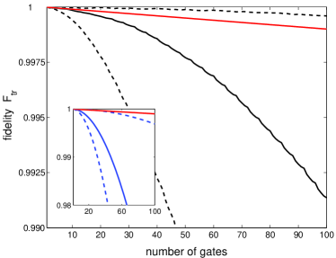
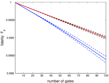
Abbildung 3: (Colour online) Comparison of error-propagation models for random unitary gates with $m=2$ qubits (a) and $m=8$ qubits (b) requiring representations with different scales. Single gate fidelity in the Monte Carlo simulations is $F_{m}=0.99999$. Repetition of the same gate $A$ (blue) is compared with repetitions of a sequence of four independent gates $ABCD$ (black). Out of 10 Monte Carlo simulations (details see text), the median (solid lines) as well as the best and worst cases (dashed lines) are given. The red solid lines denote independent error propagation $F_{\rm tr}=(F_{m})^{r}$. Large systems ($m=8$) with several gates ($ABCD$) resemble independent error propagation almost perfectly, as in (b) the black and the red solid lines virtually coincide.

Error Propagation and Relaxative Losses

As the main figure of merit we refer to a quality function

$$q:=F_{\rm tr}\;e^{-\tau/T_{R}}$$ (13)

resulting from the fidelity $F_{\rm tr}$ and the relaxative decay with overall relaxation rate constant $T_{R}$ during a duration $\tau$ assuming independence of fidelity and decay. Moreover, for $n$ qubits one defines as the trace fidelity of an experimental unitary module $U_{\rm exp}$ with respect to the target gate $V_{\rm target}$ the quantity

$$\begin{split}F_{\rm tr}&:=\;\tfrac{1}{N}\;\operatorname{Re}\;\operatorname{tr}\{V^{\dagger}_{\rm target}U^{\phantom{\dagger}}_{\rm exp}\}\\[5.69054pt] &\phantom{:}=\;1-\tfrac{1}{2N}\;\|V_{\rm target}-U_{\rm exp}\|{}_{2}^{2}\quad,\end{split}$$ (14)

where both $U,V\in U(N)$ with $N:=2^{n}$. It follows via the simple relation to the Euclidean distance

$$\begin{split}\|V-U\|{}_{2}^{2}&=\|U\|{}_{2}^{2}+\|V\|{}_{2}^{2}-2\operatorname{Re}\operatorname{tr}\{V^{\dagger}U\}\\[5.69054pt] &=2N-2N\tfrac{1}{N}\operatorname{Re}\operatorname{tr}\{V^{\dagger}U\}\\[5.69054pt] &=2N(1-F_{\rm tr})\quad,\end{split}$$

the latter two identities invoking unitarity of $U,V$. The reason for chosing the trace fidelity is its convenient Fréchet differentiability in view of gradient-flow techniques, see also Ref. Schulte-Herbrüggen et al. (2008a).

Consider an $m$-qubit-interaction module (cisc) with quality $q_{m}=F_{m}\;e^{-\tau_{m}/T_{m}}$ that decomposes into $r$ universal two-qubit gates (risc), out of which $r\,^{\prime}\leq r$ gates have to be performed sequentially. Moreover, each 2-qubit gate shall be carried out with the uniform quality $q_{2}=F_{2}\;e^{-\tau_{2}/T_{2}}$. Henceforth we assume for simplicity equal relaxation rate constants, so $T_{2}=T_{m}$ are identified with $T_{R}$. Then, as a first useful rule of the thumb and assuming independent error propagation, it is advantageous to compile the $m$-qubit module directly if $F_{m}>(F_{2})^{r}$. Or more precisely taking relaxation into account, if the module can be realised with a fidelity

$$F_{m}>(F_{2})^{r}\;e^{-(r\,^{\prime}\cdot\tau_{2}-\tau_{m})/T_{R}}\quad.$$ (15)

A more refined picture emerges from Monte-Carlo simulations of error propagation. To this end, compare the above independent error estimates with two scenarios for a sequence of $r$ gates in total: (i) the $r$-fold repetition of single unitary gates $A$ with individual errors meant to give $A^{r}$ with $r=1,2,3,\dots$ and (ii) the repetition of a sequence of four different gates $A,B,C,D$ again each with individual errors to give $(D\circ C\circ B\circ A)^{r/4}$ where $r=4,8,12,\dots$. In the sequel, we refer to case (i) as $AAAA$ and to case (ii) as $ABCD$.

(a)                                         (b)                                                                                   
     

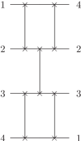
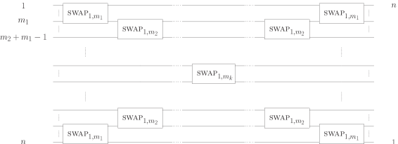
Abbildung 4: (a) Simple starting point: building a swap_1,4 gate from five swaps_1,2. (b) Generalisation: assembling a swap_1,n by four swaps${}_{1,m_{j}}$ for each type $j=1,2,\dots,k-1$ and one single swap${}_{1,m_{k}}$ so that $m_{k}+2\sum_{j=1}^{k-1}(m_{j}-1)=n$.

For gates and errors to be generic, we use random unitaries (distributed according to the Haar measure following a recent modification Mezzadri (2007) of the qr-algorithm). To a given random unitary $m$-qubit gate $A_{0}\in U(2^{m})$ (defining its Hamiltonian $H_{A0}$ via $A_{0}=e^{-iH_{A0}}$) we simulate a generic error as follows: from another independent unitary $E_{j}$ take the matrix logarithm $H_{Aj}$ such that $e^{-iH_{Aj}}=E_{j}$. Then to a given trace fidelity $F$, a corresponding unitary with a Monte-Carlo random error (the error being introduced on the level of the Hamiltonian generators) can readily be obtained by solving

$$\begin{split}F&=1-\frac{1}{2N}||A_{0}-A_{j}||_{2}^{2}\\[5.69054pt] &=1-\frac{1}{2N}\big{|}\big{|}A_{0}-e^{-i(H_{A0}+\delta\cdot H_{Aj})}\big{|}\big{|}_{2}^{2}\end{split}$$ (16)

for $\delta>0$. Along these lines one obtains the Monte-Carlo fidelities for repeating the $A$-gate by

$$F_{AAAA}(r)=1-\frac{1}{2N}\big{|}\big{|}(A_{0})^{r}-\prod\limits_{j=1}^{r}A_{j}\big{|}\big{|}_{2}^{2}$$ (17)

and

$$F_{ABCD}(r)=1-\frac{1}{2N}\big{|}\big{|}(D_{0}C_{0}B_{0}A_{0})^{\tfrac{r}{4}}-\prod\limits_{j=1}^{\tfrac{r}{4}}(D_{j}C_{j}B_{j}A_{j})\big{|}\big{|}_{2}^{2}\;,$$ (18)

where the product runs from right to left. These Monte-Carlo simulations are compared to the simple model of independent errors according to

$$F_{\rm ind}=(F_{m})^{r}\quad.$$ (19)

As shown in Fig. 3 a, for two-qubit gates the error propagates with a vast variance, which makes it virtually unpredictable. Thus assuming independence is always too optimistic for AAAA, while for ABCD it is still mostly optimistic, although there are cases in which the errors may compensate to give less effective loss than expected under independence.

However, when moving to effective multi-qubit gates, i.e., cisc modules, the generic situation becomes more predictable. For example, in $8$-qubit random unitary gates, Fig. 3 b shows that AAAA is significantly deviating from independent error propagation, whereas ABCD resembles independent error propagation almost perfectly. The situation is qualitatively exactly the same even if the single gate error is larger as tested by analogous Monte-Carlo simulations setting $F_{\rm tr}=0.99$ or $F_{\rm tr}=0.96$ (not shown).

In the sequel, we will—for the sake of simplicity—often assume independent error propagation at the expense of systematically underestimating the pros of cisc compilation compared to the standard risc compilation into universal local and two-qubit gates.

Computational Methods and Devices

Following the lines of our previous work on time complexity Schulte-Herbrüggen et al. (2005), we used the grape algorithm Khaneja et al. (2005) for direct cisc compilation. It tracks the fixed final times down to the shortest durations of controls still allowing for synthesising the unitary target gates with full fidelity. This gives currently the best known upper bounds to the minimal times required to realise a target module on a concrete hardware setting. We extended our parallelised c++ code of the grape package described in Gradl et al. (2006) by adding more flexibility allowing to efficiently exploit available parallel nodes independent of internal parameters Schulte-Herbrüggen et al. (2008b). Moreover, faster algorithms for matrix exponentials on high-dimensional systems based on approximations by Tchebychev series have been developed Waldherr (2007) specifically in view of application to large quantum systems Schulte-Herbrüggen et al. (2008b). Thus computations could be performed on the hlrb-ii supercomputer cluster at Leibniz Rechenzentrum of the Bavarian Academy of Sciences Munich. It provides an sgi Altix 4700 platform equipped with 9728 Intel Itanium2 Montecito Dual Core processors with a clock rate of $1.6$ GHz, which give a total linpack performance of $63.3$ TFlops/s. The present explorative study exploited the time allowance of approx. $500.000$ cpu hours.

I The $1,n$ SWAP Operation

         (a)                                                                   (b)                                                        
         

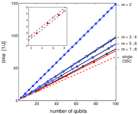
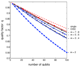
Abbildung 5: (Colour online) (a): Times required for indirect swaps_1,n on linear chains of $n$ Ising-coupled qubits by assembling swap_1,m building blocks reaching from $m=2$ (risc) up to $m=8$ (cisc). Using linear regression, the dashed line is an extrapolation of the direct single-cisc compilations shown in the inset to large number of qubits, where direct cisc compilation is virtually impossible on classical computers. Time units are expressed as $1/J_{ZZ}$ assuming the duration of local operations can be neglected compared to coupling evolutions (details in the text). (b): Translation of the effective gate times into overall quality figures $q=(q_{m})^{r_{m}}$ for an effective gate assembled from $r_{m}$ components of single qualities $q_{m}:=F_{m}\;e^{-\tau_{m}/T_{R}}$ (with the respective component fidelities homogeneously falling into a narrow interval $F_{m}\in[0.99994,0.99999]$ for $m=3,\dots,8$). Data are shown for a uniform relaxation rate constant of $1/T_{R}=0.004J_{ZZ}$.

The easiest and most basic examples to illustrate the pertinent effects of optimal-control based cisc-quantum compilation are the respective indirect swap_1,n gates in spin chains of $n$ qubits coupled by nearest-neighbour Ising interactions with $J_{ZZ}$ denoting the coupling constant.

For the swap_1,2 unit there is a standard textbook decomposition into three cnots. Thus for Ising-coupled systems and in the limit of fast local controls, the total time required for an swap_1,2 is $3/(2J_{ZZ})$, and there is no faster implementation Khaneja et al. (2001, 2002). Note, however, that in systems coupled by the isotropic Heisenberg interaction $XXX$, the swap_1,2 may be directly implemented just by letting the system evolve for a time of only $1/(2J_{XXX})$. Sacrificing universality, it may thus be advantageous to regard the swap_1,2 as basic unit for the swap_1,n task rather than the universal cnot. Clearly, any even-order swap_1,2n can be built from swaps_1,2 along the lines of the most obvious scheme of Fig. 4 a. (The odd-order swaps_1,2n-1 follow, e.g., from swap_1,2n by omitting qubit $2n$ and all the gates connected to it.)

Moreover, the generalisation to decomposing a swap_1,n into a sequence with $k$ different swap${}_{1,m_{j}}$ building blocks (where $j=1,2,\dots,k$) as shown in Fig. 4 b is straightforward by ensuring $m_{k}+2\sum_{j=1}^{k-1}(m_{j}-1)=n$. Due to its symmetry, the total duration then amounts to

$$\tau(\text{{\sc swap}}_{1,n})=\tau(\text{{\sc swap}}_{1,m_{k}})+2\sum\limits_{j=1}^{k-1}\tau(\text{{\sc swap}}_{1,m_{j}})$$ (20)

and the overall quality as a function of the fidelities of the constitutent gates reads

$$\begin{split}q_{\text{{\sc swap}}_{1,n}}=F(\text{{\sc swap}}_{1,m_{k}})&\quad\prod\limits_{j=1}^{k-1}F(\text{{\sc swap}}_{1,m_{j}})^{4}\\ &\times e^{-\tau(\text{{\sc swap}}_{1,n})/T_{R}}\quad.\end{split}$$ (21)

Now, the swap${}_{1,m_{j}}$ building blocks themselves can be precompiled into time-optimised single complex instruction sets by exploiting the grape-algorithm of optimal control up to the current limits of $m_{j}$ imposed by cpu-time allowance.

Proceeding in the next step to large $n$, Fig. 5 underscores how the time required for swap_1,n gates decreases significantly by assembling precompiled swap${}_{1,m_{j}}$ building blocks as cisc units recursively up to a multi-qubit interaction size of $m_{j}=8$, where the speed-up is by a factor of nearly $2$. Clearly, such a set of swap${}_{1,m_{j}}$ building blocks with $m_{j}\in\{2,3,4,5,6,7,8\}$ allows for efficiently synthesising any swap_1,n. Assuming for the moment that a linear time complexity of the swap_1,n can be taken for granted, one may extrapolate the results of direct cisc compilation from the range of the inset of Fig. 5 a to a large number of qubits. One thus obtains an estimated upper limit to the time complexity of the swap_1,n. This is indicated by the dashed line, the slope of which will be defined as $\Delta_{\infty}$. Likewise, the irrespective slopes of the $m$-qubit decomposition are denoted by $\Delta_{m}$.

With these stipulations, we introduce as a measure for the potential of cisc compilation (versus risc compilation) the ratio of the slopes

$$\pi_{\text{\sc cisc}}:=\frac{\Delta_{2}}{\Delta_{\infty}}$$ (22)

and as a measure for the extent to which this potential has been exhausted by $m$-qubit cisc compilation the ratio

$$\eta_{m}:=\frac{\Delta_{\infty}}{\Delta_{m}}$$ (23)

thus providing as convenient measure of improvement

$$\xi_{m}:=\frac{\Delta_{2}}{\Delta_{m}}=\eta_{m}\cdot\pi_{\text{\sc cisc}}\quad.$$ (24)

The data of Fig. 5 thus give a potential of $\pi_{\text{\sc cisc}}=2.16$; by $m=8$-qubit interactions it is already pretty well exhausted, as inferred from $\eta_{8}=0.87$. The current cisc over risc improvement then amounts to $\xi_{8}=1.88$.

On the other hand, deducing from Fig. 5 right away that the time complexity of swaps_1,n ought to be linear would be premature: although the slopes seem to converge to a non-zero limit, numerical optimal control may become systematically inefficient for larger interaction sizes $m$. Therefore, although improbable, e.g., convergence of the slopes to a value of zero cannot be safely excluded on the current basis of findings. This also means a logarithmic time complexity can ultimately not be excluded either.

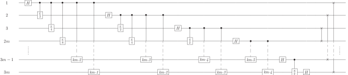
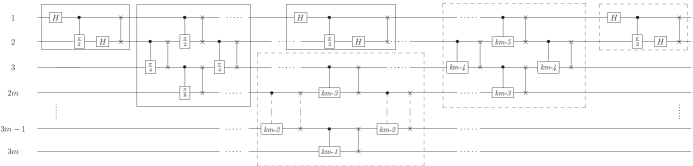
Abbildung 6: By rearranging the swaps and controlled phase gates, the standard decomposition of a $3m$-qubit quantum Fourier transform, qft (top trace) reduces to a realisation adapted to a coupling topology of linear nearest-neighbour interactions (lower trace) with a $2m$-qubit qft, $m$-qubit cp-swaps (solid boxes), and an $m$-qubit qft (dashed box). The notation $(km-\nu)$ is a shorthand for a rotation angle of $\phi=\frac{\pi}{2^{km-\nu}}$.

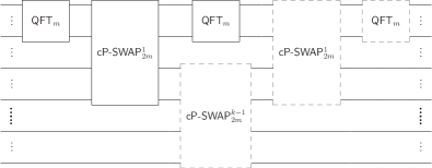
Abbildung 7: For $k\geq 2$, a $(km)$-qubit qft can be assembled from $k$ times an $m$-qubit qft and $k\choose 2$ instances of $2m$-qubit modules cp-swap${}_{2m}^{j}$, where the index $j$ of different phase-rotation angles takes the values $j=1,2,\dots,k-1$. The dashed boxes correspond to Fig. 6 and show the induction $k\mapsto k+1$.

Summarising the results for the indirect swaps in terms of the three criteria described in the introduction, we have the following: (i) in Ising coupled qubit chains, there is no speed-up by changing the basic unit from the universal cnot into a swap_1,2, whereas in isotropically coupled systems the speed-up amounts to a factor of three; (ii) extending the building blocks of swap_1,m from $m=2$ (risc) to $m=8$ (cisc) gives a speed-up by a factor of nearly two under Ising-type couplings; (iii) the numerical data are consistent with a time complexity converging to a linear limit for the swap_1,n task in Ising chains, however, there is no proof for it yet.

II The Quantum Fourier Transform (QFT)

Since many quantum algorithms take advantage of efficiently solving some hidden subgroup problem, the quantum Fourier transform plays a central role Jozsa (1998); Cleve et al. (1998); Ettinger et al. (2004).

In order to realise a qft on large qubit systems, our approach is the following: given an $m$-qubit qft, we show that for obtaining a $(k\cdot m)$-qubit qft by recursively using multi-qubit building blocks, a second type of module is required, to wit a combination of controlled phase gates and swaps, which henceforth we dub $m^{\prime}$-qubit cp-swap for short.

                   (a)                                                                       (b)                                                        

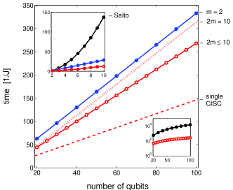
Abbildung 8: (Colour online) Comparison of cisc-compiled qft (red) with standard risc compilations ($m=2$) following the scheme by Saito Saito et al. (2000) (black) or Blais Blais (2001) (blue): (a) times for implementation translate into quality factors (b) for a relaxation rate constant of $1/T_{R}=0.004J_{ZZ}$. Again, the dashed red line extrapolates from the direct single-cisc compilations shown in the upper inset of (a), the lower inset giving in logarithmic scales the times needed for the standard textbook risc compilation ($m=2$) on a linear Ising chain. Dotted red lines represent the less favourable results from qft variant II (Appendix A).

Here we present two alternatives: variant I with $m^{\prime}=2m$ and, as a special case, variant II for even $m^{\prime}=m$.

Choosing $m=2$ and $k=3$ for a start, the recursive construction is illustrated in Fig. 6. The top trace shows the standard textbook realisation of a $6$-qubit qft. By shifting the final swap operations, it can be rearranged into the sequence of gates depicted in the lower trace. Note that the gates appearing in solid boxes constitute a $2m$-qubit qft (which itself is made of two $m$-qubit qfts and a central $m$-qubit cp-swap), while the ones in dashed boxes have to be added for a $3m$-qubit qft. For $m=2$ we have thus shown how a $3m$-qubit qft reduces to a $2m$-qubit qft, two $2m$-qubit cp-swaps, and an $m$-qubit qft. So with $2m$ providing a foundation, at the same time we have also illustrated the induction from a $k\cdot m$-qft to a $(k+1)\cdot m$-qft. Moreover, the same construction principle holds for any block size $m=2,3,\dots$, which can readily be proven by a straightforward, but lengthy induction from $m$ to $m+1$.

One thus arrives at the desired block decomposition of a general $(k\cdot m)$-qubit qft as shown in Fig. 7 (which is variant I; the less effective variant II can be found in Appendix A): it requires $k$ times the same $m$-qubit qft interdispersed with $k\choose 2$ times an $2m$-qubit cp-swap, out of which $k-1$ show different phase-roation angles. For all $m$ and $j=1,2,\dots,(k-1)$, one finds the following observations:

1. a cp-swap${}_{2m}^{j}$ takes as least as long as a qft_m;

2. a qft_m takes as least as long as a cp-swap${}_{m}^{j}$;

3. a cp-swap${}_{m}^{j}$ takes least as long as a cp-swap${}_{m}^{j+1}$ .

Thus the duration of a $(k\cdot m)$-qubit qft built from $m$-qubit and $2m$-qubit modules amounts to

$$\begin{split}\tau(\text{\sc qft}_{k\cdot m})=2\cdot&\tau(\text{\sc qft}_{m})+(k-1)\cdot\tau(\text{c{\sc p-swap}}_{2m}^{1})\\ &+(k-2)\cdot\tau(\text{c{\sc p-swap}}_{2m}^{2})\quad.\end{split}$$ (25)

Next, consider the overall quality of a $(k\cdot m)$-qubit qft in terms of its two types of building blocks, namely the basic $m$-qubit qft as well as the constituent $2m$-qubit cp-swaps with their respective different rotation angles. It reads

$$\begin{split}q_{\text{\sc qft}_{k\cdot m}}=\;(F_{\text{\sc qft}_{m}})^{k}\;\big{(}\prod\limits_{j=1}^{k-1}&\;(F_{\text{c{\sc p-swap}}_{2m}^{j}})^{k-j}\;\big{)}\\ &\qquad\times\;e^{-(\tau_{\text{\sc qft}_{k\cdot m}}/T_{R})}\,.\end{split}$$ (26)

In the following, we will neglect rotations as soon as their angle falls short of a threshold of $\pi/2^{10}$. This approximation is safe since it is based on a calculation of a $20$-qubit qft, where the truncation does not introduce any relative error beyond $10^{-5}$. According to the block decomposition of Fig. 7, thus three instances of cp-swaps are left, since all cp-swap${}_{10}^{j}$ elements with $j\geq 3$ boil down to mere swap gates due to truncation of small rotation angles. The representation of these cp-swap modules is shown in Appendix B as Fig. 17.

With these stipulations, we address the task of assembling an $(k\cdot 10)$-qubit qft, exploiting the limits of current allowances on the hlrb-ii cluster. This translates into using $10$-qubit cp-swap building blocks ($2m=10$) and the $5$-qubit qft ($m=5$) in the sense of a $(2k\cdot 5)$-qubit qft. Its duration $\tau(\text{\sc qft}_{2k\cdot 5})$ is readily obtained as in Eqn. 25 thus giving an overall quality of

$$\begin{split}q_{\text{\sc qft}_{2k\cdot 5}}=\;&(F_{\text{\sc qft}_{5}})^{2k}\;(F_{\text{c{\sc p-swap}}_{10}^{1}})^{2k-1}\;(F_{\text{c{\sc p-swap}}_{10}^{2}})^{2k-2}\\ &\times\;\,(F_{\text{c{\sc p-swap}}_{10}^{3}})^{{2k\choose 2}-4k+3}\quad e^{-\tau_{\text{\sc qft}_{2k\cdot 5}}/T_{R}}\,.\end{split}$$ (27)

Based on this relation, the numerical results of Fig. 8 show that a cisc-compiled qft is moderately superior to the standard risc versions Saito et al. (2000); Blais (2001). Although the potential of cisc compilation amounts to $\pi_{\text{\sc cisc}}=2.27$, recursively assembling $5$-qubit qfts and $10$-qubit cp-swaps only exploits about half of it as apparent in the value of $\eta^{\phantom{|}}_{5,10}=0.53$.

As has been pointed out by Zeier Zeier (2007), the decomposition of a many-qubit qft into smaller qfts and concatenations of a permutation matrix and a diagonal matrix roots back in a principle already used in the Cooley-Tukey algorithm Cooley and Tukey (1965) for the discrete Fourier transform (dft): Let $N=m\cdot q$. Then one obtains Clausen and Baum (1993); Egner (1997)

$$\begin{split}\text{\sc dft}_{N}&=L\circ(\text{\sc dft}_{m}\otimes{\rm 1\negthickspace l}{}_{q})\circ D\circ({\rm 1\negthickspace l}{}_{m}\otimes\text{\sc dft}_{q})\\ &=({\rm 1\negthickspace l}{}_{q}\otimes\text{\sc dft}_{m})\circ(L\circ D)\circ({\rm 1\negthickspace l}{}_{m}\otimes\text{\sc dft}_{q})\;,\end{split}$$ (28)

where $L\in\operatorname{Mat}{}_{N}$ is a permutation matrix. Moreover, setting $\omega:=e^{2\pi i/N}$, the diagonal matrix takes the form

$$D=\operatorname{diag}{}(\omega^{t_{k}}|t_{k}=(k\operatorname{mod}{\;}m)\lfloor\tfrac{k}{m}\rfloor\;\text{for}\;k=0,1,2,\dots N-1)$$ (29)

Therefore, the qft decompositions made use of here exactly follow the classical scheme in the second line of Eqn. 28, the expression $(L\circ D)$ corresponding to the cp-swap.

III The Multiple-Controlled NOT Gate (CⁿNOT)

Multiply-controlled cnot gates generalise Toffoli’s gate. Here, we move from c²not to c^n-2not in an $n$-qubit system with one ancilla and one target qubit. The reason for the ancilla qubit being that it turns the problem to linear complexity Barenco et al. (1995). Moreover, in view of realistic large systems, we assume again a topology of a linear chain coupled by nearest-neighbour Ising interactions. Since c^mnot-gates frequently occur in error-correction schemes, they are highly relevant in practice.

Here we address the task of decomposing a c^n-2not into lower cnots and indirect swap gates (see Sec. I).

To this end, we will generalise the basic principle of reducing a cⁿnot to c^mnot gates with $m<n$ that can be demonstrated by decomposing a c³not into Toffoli gates according to scheme of Fig. 9 devised by Barenco et al. in Barenco et al. (1995). Starting with any of the $2^{5}$ computational basis states $|x_{1},x_{2},x_{3},x_{4},x_{5}\rangle{}$ (where $x_{k}\in\{0,1\}$, $\oplus$ denotes addition $\operatorname{mod}{\;}2$, and $x_{k}x_{\ell}$ being the usual scalar product) track the effect of the gate sequentially from state $|a\rangle{}$ through state $|e\rangle{}$

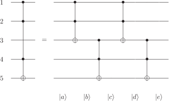
Abbildung 9: Decomposition of a $C^{3}$-NOT with one ancilla qubit into four $C^{2}$-NOTs (Toffoli gates) according to ref. Barenco et al. (1995). States $|a\rangle{}$ through $|e\rangle{}$ are explained in the text.

1. $=|x_{1},x_{2},x_{3},x_{4},x_{5}\rangle{}$

2. $=|x_{1},x_{2},x_{3}\oplus x_{1}x_{2},x_{4},x_{5}\rangle{}$

3. $=|x_{1},x_{2},x_{3}\oplus x_{1}x_{2},x_{4},x_{5}\oplus x_{4}(x_{3}\oplus x_{1}x_{2})\rangle{}$
   $=|x_{1},x_{2},x_{3}\oplus x_{1}x_{2},x_{4},x_{5}\oplus x_{4}x_{3}\oplus x_{1}x_{2}x_{4}\rangle{}$

4. $=|x_{1},x_{2},x_{3}\oplus x_{1}x_{2}\oplus x_{1}x_{2},x_{4},x_{5}\oplus x_{4}x_{3}\oplus x_{1}x_{2}x_{4}\rangle{}$
   $=|x_{1},x_{2},x_{3},x_{4},x_{5}\oplus x_{4}x_{3}\oplus x_{1}x_{2}x_{4}\rangle{}$

5. $=|x_{1},x_{2},x_{3},x_{4},x_{5}\oplus x_{4}x_{3}\oplus x_{4}x_{3}\oplus x_{1}x_{2}x_{4}\rangle{}$
   $=|x_{1},x_{2},x_{3},x_{4},x_{5}\oplus x_{1}x_{2}x_{4}\rangle{}$

to see the overall effect of the gate sequence is a c³not thus proving the decomposition.

(a)                                                            (b)
  

$*$                                    $*$

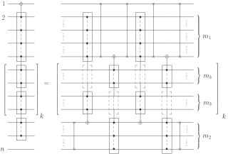
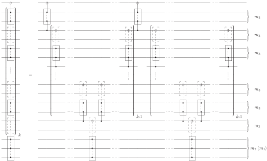
Abbildung 10: Decomposition of a c^n-2not gate on a linear coupling topology: (a) reduction of the number of control qubits to four intermediate gates with fewer control qubits and (b) decomposition of the intermediate multiply-controlled not-gate appearing in (a). In an $n$-qubit system, there is one target qubit, one ancilla qubit and $n-2$ control qubits; so $m_{1}+(m_{2}-1)+2km_{3}=n-2$ with $m_{1},m_{3}\geq 1$ and $m_{2}\geq 2$. Read the brackets $[\cdot]_{k}$ in (a) as to be expanded $k$ times and $(\cdot)_{k}$ in (b) as expanded $k$-fold.

(a)                                                                        (b)

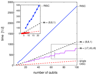
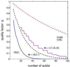
Abbildung 11: (Colour online) Comparing implementations of c^n-2nots on a linear Ising spin chain using cnot and swap_1,2 modules for the risc compilation or multi-qubit building blocks according to the cisc assembler scheme of Fig. 10. As a short-hand, the different numbers of control qubits are expressed by $\mathbf{m}:=(m_{1},m_{2},m_{3})$. Using the expansion of Fig. 10, the cisc results (black solid lines) are obtained for $k=4,5,6,\dots$ with $m_{1}=8$ and $m_{2}=8$ (for odd $n$) or $m_{2}=7$ (for even $n$), while $m_{3}=1$ thus ensuring $m_{1}+(m_{2}-1)+2km_{3}=n-2$. The red dotted line extrapolates again the direct cisc results beyond 10 qubits. In (a) deviations from straight lines occur, as the cases $k=1,2,3$ follow special concatenation patterns (see text), while $k=4,5,6,\dots$ are generic. The inset in (a) also shows results of a non-scalable recursive expansion that is confined up to $19$ qubits (blue circles). The step functions with periods indicated by tags represent a faster alternative explained in the next section, where the boxed part of trace (a) is blown up in Fig. 15.

Fig. 10 provides a generalisation of the scheme in Fig. 9: in the first place (a), the number of control qubits is reduced by introducing $k$ blocks with $m_{3}$ qubits that are left invariant. The price for this reduction is a four-fold occurence of the reduced building blocks. In the second step (b), the reduced building blocks are expanded into a sequence with two central c${}^{m_{2}}$nots, two terminal c${}^{(m_{3}+1)}$nots and two lots of $2(k-1)$ times c${}^{(m_{3}+1)}$not each. For $k=4,5,6,\dots$ part (a) and (b) can be expanded in a general concatenated way thus entailing an overall duration of

$$\begin{split}\tau(&\text{\sc c}^{n-2}\text{\sc not})\Big{|}_{k\geq 4}\;=\;4\tau(\text{\sc c}^{m_{1}}\text{\sc not})\\[5.69054pt] &+4\tau(\text{\sc c}^{m_{2}}\text{\sc not})+\tau(\text{{\sc swap}}_{1,m_{2}})\\[5.69054pt] &+(13k-8)\tau(\text{\sc c}^{m_{3}+1}\text{\sc not})\\[5.69054pt] &+(1-\delta_{m_{3},1})\;(13k+3)\tau(\text{{\sc swap}}_{1,m_{3}})\;.\\[5.69054pt] \end{split}$$ (30)

For completeness, note that the cases $k=3,2,1$ have to be treated separately, since they only allow for less and less densly concatenated expansions (not shown). Their respective durations are

$$\begin{split}\tau(&\text{\sc c}^{n-2}\text{\sc not})\big{|}_{k=1}\;=\;4\tau(\text{\sc c}^{m_{1}}\text{\sc not})+2\tau(\text{{\sc swap}}_{1,m_{1}+1})\\[1.42262pt] &+4\tau(\text{\sc c}^{m_{2}}\text{\sc not})+2\tau(\text{{\sc swap}}_{1,m_{2}})\\[1.42262pt] &+8\tau(\text{\sc c}^{m_{3}+1}\text{\sc not})+(1-\delta_{m_{3},1})\;16\tau(\text{{\sc swap}}_{1,m_{3}})\\[5.69054pt] \end{split}$$ (31)

$$\begin{split}\tau(&\text{\sc c}^{n-2}\text{\sc not})\big{|}_{k=2}\;=\;4\tau(\text{\sc c}^{m_{1}}\text{\sc not})\\[1.42262pt] &+4\tau(\text{\sc c}^{m_{2}}\text{\sc not})+\tau(\text{{\sc swap}}_{1,m_{2}})\\[1.42262pt] &+24\tau(\text{\sc c}^{m_{3}+1}\text{\sc not})+(1-\delta_{m_{3},1})\;32\tau(\text{{\sc swap}}_{1,m_{3}})\\[5.69054pt] \end{split}$$ (32)

$$\begin{split}\tau(&\text{\sc c}^{n-2}\text{\sc not})\big{|}_{k=3}\;=\;4\tau(\text{\sc c}^{m_{1}}\text{\sc not})\\[1.42262pt] &+4\tau(\text{\sc c}^{m_{2}}\text{\sc not})+\tau(\text{{\sc swap}}_{1,m_{2}})\\[1.42262pt] &+37\tau(\text{\sc c}^{m_{3}+1}\text{\sc not})+(1-\delta_{m_{3},1})\;48\tau(\text{{\sc swap}}_{1,m_{3}})\;.\\[5.69054pt] \end{split}$$ (33)

However, the total number of gates only depends on $k=1,2,3,\dots$, so that obtains as the overall quality

$$\begin{split}q\big{|}_{k}\;=\;&(F_{C^{m_{1}}NOT})^{4}(F_{\text{{\sc swap}}_{1,m_{1}+1}})^{4}\\[2.84526pt] &\times(F_{C^{m_{2}}NOT})^{4}(F_{\text{{\sc swap}}_{1,m_{2}}})^{2}\\[2.84526pt] &\times(F_{C^{m_{3}+1}NOT})^{16k-8}\;(F_{\text{{\sc swap}}_{1,m_{3}}})^{(1-\delta_{m_{3},1})\,16k}\\[2.84526pt] &\times e^{-\tau(C^{n-2}NOT)\big{|}_{k}/T_{R}}\;.\end{split}$$ (34)

Given the duration of the decomposition as in Eqn. 30, it is easy to see that implementing the $m_{1}$ control qubits comes with the lowest time weight (4) and without a time overhead of auxiliary gates. Implementing the $m_{2}$ control qubits, however, requires the same time weight (4), but entails the time for one auxiliary swap${}_{1,m_{2}}$ gate. In order to implement the $k\cdot m_{3}$ control qubits, in turn, a sizeable amount of auxiliary swaps are needed.

Therefore, whenever high fidelities can be reached (so that the quality is limited by relaxation not by fidelity), a good strategy of combining the expansive decomposition in Fig. 10 a with the recursive decomposition in part (b) is the following: given $n-2$ control qubits and with the current limitation from direct cisc compilation being $m_{j}\leq 9$, choose $m_{1}$ to be the largest, $m_{2}$ to be the second largest and such that one obtains an even number for $n-m_{1}-m_{2}-1=2km_{3}$.

In the next step, a decision has to be made in order to minimise the contributions in the last two lines of Eqn. 30, whenever there are several integer solutions $km_{3}=k^{\prime}m_{3}^{\prime}$. So for integer $k\geq 4$, this amounts to the ordinary minimisation task

$$\begin{split}\underset{k}{\min}\;(13k-8)&\,\{(m_{3}+2)\Delta_{C}+a\}\\ &\qquad+(1-\delta_{m_{3},1})\;(13k+3)\,\{m_{3}\Delta_{S}+b\}\\[5.69054pt] \text{subject to:}\quad&km_{3}=\text{const.}\equiv\frac{n-(m_{1}+m_{2}+1)}{2}\end{split}$$ (35)

Here we approximate the times for a c${}^{m_{3}+1}$not by the linear expression $\tau(\text{\sc c}^{m_{3}+1}\text{\sc not})=(m_{3}+2)\Delta_{C}+a$ and likewise for the swap${}_{1,m_{3}}$ by $\tau(\text{{\sc swap}}_{1,m_{3}})=m_{3}\Delta_{S}+b$ with the values for the slopes $\Delta_{C},\Delta_{S}$ and the offsets $a$ and $b$ being taken from the respective linear regression for extrapolating $\Delta_{\infty}$ for direct cisc compilation ($\Delta_{C}^{(\infty)}=2.15$ and $\Delta_{S}^{(\infty)}=0.69$ as well as $a=-4.48$ and $b=0.06$). In the setting of these parameters, Eqn. 30 implies it is timewise advantageous to choose as the decomposition of the interior block in Fig. 10 b the counter-intuitive option with a large number $k$ of small block sizes $m_{3}$. This is because in the above parameter setting, the duration takes its minimum on the margin circumventing the time overhead skipped by $(1-\delta_{m_{3},1})=0$ thus giving high repetitions $k=\frac{n-(m_{1}+m_{2}+1)}{2}$ and smallest block sizes $m_{3}=1$ corresponding to Toffoli gates. The speed-up is illustrated in Fig. 11: although it amounts to a factor of $2.45$ compared to the standard risc decomposition, the potential as extrapolated from direct cisc compilation up to nine qubits gives a lower bound for the speed-up by $13.6$.

Faster Alternatives of $\text{\sc c}^{n-2}\text{\sc not}$

Since the potential of cisc compiling cⁿnot gates is largely not yet exploited by the previous scheme, it is worth showing a faster scalable decomposition at the expense of being more elaborate. To this end, we proceed in two steps, first we show the general principle of an auxiliary backbone gate, namely an indirect cnot between qubit 1 and some distant qubit $\ell+1$ (which may be separated by $\ell$ intermediate qubits, e.g., in a linear coupling topology). Second we implement the resulting faster alternative into Fig. 10 b.

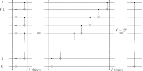
Abbildung 12: Principle of generating an indirect cnot by restricting $\ell=2^{p}$ as described in the text.

Fig. 12 shows the principle identities: if $\ell$ is an integer power of two, the two identities hold for any $\ell=2^{p}$. The second identity is easy to see since the ascending series of cnot gates can be represented by a Jordan matrix over the field of binary numbers $\mathbb{Z}_{2}^{\ell+1}:=\{0,1\}^{\ell+1}$ with the addition modulo $2$ so as to take the form

$$(J)_{\mathbb{Z}_{2}^{\ell+1}}=\begin{pmatrix}1&1&0&0&\cdots&0&0&0\\ 0&1&1&0&\cdots&0&0&0\\ 0&0&1&1&\cdots&0&0&0\\ 0&0&0&1&\cdots&0&0&0\\ \vdots&&&&\ddots&&&\vdots\\ 0&0&0&0&\cdots&1&1&0\\ 0&0&0&0&\cdots&0&1&1\\ 0&0&0&0&\cdots&0&0&1\end{pmatrix}^{t}\;.$$ (36)

In terms of natural numbers, its $\ell^{\rm th}$ power reads

$$J^{\ell}=\begin{pmatrix}1&\binom{\ell}{1}&\binom{\ell}{2}&\binom{\ell}{3}&\cdots&\binom{\ell}{\ell-2}&\binom{\ell}{\ell-1}&\binom{\ell}{\ell}\\[2.84526pt] 0&1&\binom{\ell}{1}&\binom{\ell}{2}&\cdots&\binom{\ell}{\ell-3}&\binom{\ell}{\ell-2}&\binom{\ell}{\ell-1}\\[2.84526pt] 0&0&1&\binom{\ell}{1}&\cdots&\binom{\ell}{\ell-4}&\binom{\ell}{\ell-3}&\binom{\ell}{\ell-2}\\[2.84526pt] 0&0&0&1&\cdots&\binom{\ell}{\ell-5}&\binom{\ell}{\ell-4}&\binom{\ell}{\ell-3}\\[2.84526pt] \vdots&&&&\ddots&&&\vdots\\[2.84526pt] 0&0&0&0&\cdots&1&\binom{\ell}{1}&\binom{\ell}{2}\\[2.84526pt] 0&0&0&0&\cdots&0&1&\binom{\ell}{1}\\[2.84526pt] 0&0&0&0&\cdots&0&0&1\end{pmatrix}^{t}\;.$$ (37)

For $\ell=2^{p}$ with $p=1,2,3,4,\dots$ it gives the desired indirect $\text{\sc c}^{1,\ell+1}\text{\sc not}$ as seen in the representation over $\mathbb{Z}_{2}^{\ell+1}$

$$(J^{\ell})_{\mathbb{Z}_{2}^{\ell+1}}=\begin{pmatrix}1&0&0&0&\cdots&0&0&1\\ 0&1&0&0&\cdots&0&0&0\\ 0&0&1&0&\cdots&0&0&0\\ 0&0&0&1&\cdots&0&0&0\\ \vdots&&&&\ddots&&&\vdots\\ 0&0&0&0&\cdots&1&0&0\\ 0&0&0&0&\cdots&0&1&0\\ 0&0&0&0&\cdots&0&0&1\end{pmatrix}^{t}=(\text{\sc c}^{1,\ell+1}\text{\sc not})^{t}_{\mathbb{Z}_{2}^{\ell+1}}\;.$$ (38)

This is because due to a theorem by Lucas Lucas (1878) only for $\ell$ being an integer power of two, all the binomial coefficients $\binom{\ell}{j}$ with $j=1,2,\dots,(\ell-1)$ are even, while $\binom{\ell}{0}=\binom{\ell}{\ell}=1$. They are therefore the only ones not to vanish in the representation over $\mathbb{Z}_{2}^{\ell+1}$.

The principle backbone summerised in the identities of Fig. 12 may then be extended for more general purposes: (1) Without changing $\ell$ one may insert further control qubits in the sense of replacing any cnot by a Toffoli or a higher $\text{\sc c}^{m}\text{\sc not}$. (2) Likewise, one may formally insert further target qubits to be flipped so that the not component is performed on more than one qubit. These two extensions enable a faster alternative for decomposing the module of Fig. 10 a than given in Fig. 10 b. This alternative is shown in Fig. 13 a. Due to the backbone scheme of Fig. 12, the only constraint is that ‘1 plus the number of neutral blocks of size $m_{3,j}$ (represented by dashed boxes in Fig. 13 a)´ equals $\ell=2^{p}$ with $p\in\mathbb{N}{}$’. Changing the assembly of a $\text{\sc c}^{n-2}\text{\sc not}$ from the scheme of Fig. 10 to the alternative of Fig. 13 follows by identifying $k=\ell-1=2^{p}-1$, i.e.

$$\begin{split}n-2&=m_{1}+(m_{2}-1)+2km_{3}\\[5.69054pt] &=m_{1}+(m_{2}-1)+\sum\limits_{j=1}^{2(2^{p}-1)}m_{3,j}\quad,\end{split}$$ (39)

where we explicitly allow for individual block sizes $m_{3,j}$.

(a)                    (b)

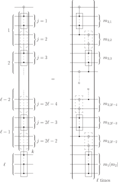
Abbildung 13: (a) Alternative decomposition of the constituent module of Fig. 10 a. The qubits tagged by the numbers $1,2,\dots,\ell$ relate to the neutral qubits of Fig. 12. (b) Each auxiliary building block involves a solid box containing $m_{3,j+1}$ control qubits and a dashed box containing $m_{3,j}$ spacer qubits. It is termed $\text{\sc c}^{(1+m_{3,j+1})}\text{\sc not}^{({m_{3,j}})}$ and its realisation is shown in Fig. 14.

As shown in Fig. 13 b, the decomposition of $m_{3,j+1}$ control qubits (solid boxes) and $m_{3,j}$ spacer qubits (dashed boxes) leads to an auxiliary gate, which we term $\text{\sc c}^{(1+m_{3,j+1})}\text{\sc not}^{({m_{3,j}})}$. It can be realised as in Fig. 14. Note that the construction scheme of Fig. 10 a requires to each solid box an equally sized dashed box.

In order to express the overall duration, we need the following notation: let the array $\vec{m}_{3}:=(\vec{m}_{3}^{1},\vec{m}_{3}^{2},\vec{m}_{3}^{3},\vec{m}_{3}^{4})$ of total length $2\ell-2$ comprise the box sizes $m_{3,j}$ of Fig. 13 b grouped into the four subsets

• sizes of the $\tfrac{\ell}{2}$ solid boxes on the left,

• sizes of the $\tfrac{\ell-2}{2}$ solid boxes on the right,

• sizes of the $\tfrac{\ell}{2}$ dashed boxes on the left, and

• sizes of the $\tfrac{\ell-2}{2}$ dashed boxes on the right,

and let $\overline{m_{3}^{s}}$ be the largest entry in $\vec{m}_{3}^{s},s=1,2,3,4$. Then the duration of the decomposition of a $\text{\sc c}^{n-2}\text{\sc not}$-gate of Fig. 10 a according to Fig. 13 and 14 reads

$$\begin{split}\tau(\text{\sc c}^{n-2}\text{\sc not})=&\phantom{;+}2\cdot 2^{p}{\Big{(}}\tau(\text{\sc c}^{\overline{m_{3}^{1}}+1}\text{\sc not})+\tau(\text{\sc c}^{\overline{m_{3}^{2}}+1}\text{\sc not})\\ &\qquad\qquad\quad\;\;+2\operatorname{max}(\overline{m_{3}^{3}},\overline{m_{3}^{4}})\cdot\tau(\text{{\sc cnot}}){\Big{)}}\\ &+2\cdot 2^{p}{\Big{(}}\tau(\text{\sc c}^{\overline{m_{3}^{3}}+1}\text{\sc not})+\tau(\text{\sc c}^{\overline{m_{3}^{4}}+1}\text{\sc not})\\ &\qquad\qquad\quad\;\;+2\operatorname{max}(\overline{m_{3}^{1}},\overline{m_{3}^{2}})\cdot\tau(\text{{\sc cnot}}){\Big{)}}\\ &+\tau_{\text{\sc swap}_{1,m_{2}}}\;.\end{split}$$ (40)

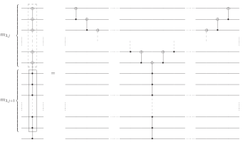
Abbildung 14: Realisation of the auxiliary building block involving several not actions.

Obviously Eqn. 40 is symmetric under the exchanges $\overline{m_{3}^{1}}\leftrightarrow\overline{m_{3}^{2}}$ and $\overline{m_{3}^{3}}\leftrightarrow\overline{m_{3}^{4}}$, while the $\operatorname{max}$-functions break a full symmetry that would also require invariance under $\overline{m_{3}^{1}}\leftrightarrow\overline{m_{3}^{3}}$ and $\overline{m_{3}^{2}}\leftrightarrow\overline{m_{3}^{4}}$. Consequently, the broken symmetry imposes rules how to increase the box sizes in a time saving way. However, since the duration is limited by the largest box size in each time slot (left part and right part in Fig. 13 b), one can fill the left and the right slots sequentially.

Given $n-2$ control qubits, a time saving decomposition of a $\text{\sc c}^{n-2}\text{\sc not}$ results by following the subsequent rules: calculate the auxiliary variables $p^{\prime}:=\lfloor\log_{2}(n-1)\rfloor-1$ and $r:=(n-1)-2^{p^{\prime}+1}$ to determine $p$ as

1. $\mathbf{p=p^{\prime}-1}$ for $p^{\prime}\geq 2$ and $r\in[1,2^{p^{\prime}-2}]$ entailing $m_{3,j}\in\{2,3\}$ and the jump at half width within step I (see Fig. 15);

2. $\mathbf{p=p^{\prime}-2}$ for $p^{\prime}\geq 3$ and $r\in[1+2^{p^{\prime}-1},5\cdot 2^{p^{\prime}-3}]$ entailing $m_{3,j}\in\{5,6\}$ and the minor jump at quarter width within step II (Fig. 15);

3. $\mathbf{p=p^{\prime}}$ otherwise; then $m_{3,j}\in\{1,2\}$.

4. NB: for $p=p^{\prime}-3$ blocksizes would increase to $m_{3,j}\in\{8,9\}$ leading to $\text{\sc c}^{9}\text{\sc not}$ and $\text{\sc c}^{10}\text{\sc not}$ building blocks, which are currently out of reach.

Then a time-saving decomposition obeys the final rule

1. Once $p$ and the box sizes $m_{3,j}\in\{b,b+1\}$ are fixed, arrange the vector of grouped sizes

   $$\begin{split}\vec{m}_{3}&:=(\vec{m}_{3}^{1},\vec{m}_{3}^{2},\vec{m}_{3}^{3},\vec{m}_{3}^{4})\\ &=(b+1,b+1,\dots,b+1,b,b,\dots,b,b)\end{split}$$

   with the entries in descending order.

Clearly, the duration will not increase as long as all entries $(b+1)$ fall into $\vec{m}_{3}^{1}$, where one may choose to start on top of Fig. 13. A time-step will occur as soon as the first $(b+1)$ falls into $\vec{m}_{3}^{2}$, which neither affects $\operatorname{max}(\overline{m_{3}^{1}},\overline{m_{3}^{2}})$ nor $\operatorname{max}(\overline{m_{3}^{3}},\overline{m_{3}^{4}})$. Analogous features hold for filling $\vec{m}_{3}^{3}$ and $\vec{m}_{3}^{4}$. They bring about the periodic step function shown in Fig. 11. Its details are given in Fig. 15, where the jump within step I is due to rule 1, while the minor jump within step II has its roots in rule 2 above.

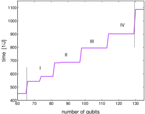
Abbildung 15: (Colour online) Detailed blow-up of the box in Fig. 11. The step function is a periodic repetition of steps I-IV, where the length of the steps (in units of numbers of qubits) doubles with every period as indicated by the tags in Fig. 11. The small jumps within steps I and II are explained in the text.

For illustration, consider the following three cases:

Example 1

In a system of $n=41$ qubits a $\text{\sc c}^{39}\text{\sc not}$ with one auxiliary qubit gives $p^{\prime}=4$. By $r=8$ rule 3 applies and $p=4$. Eqn. 39 and rule 5 then yield $\vec{m}_{3}^{1}=(2)_{8}$ and $\vec{m}_{3}^{3}=(1)_{8}$, while $\vec{m}_{3}^{2}=\vec{m}_{3}^{4}=(1)_{7}$ and $m_{1}=m_{2}=1$. Hence the time-saving decomposition involves just cnot and Toffoli gates (beyond the auxiliary cnot and indirect swap gates).

Example 2

Yet for $n=42$ qubits a $\text{\sc c}^{40}\text{\sc not}$ gives $p^{\prime}=4$ and $r=9\in[1+2^{p^{\prime}-2},5\cdot 2^{p^{\prime}-4}]=[9,10]$, so rule 2 applies and yields $p=2$. By Eqn. 39 and rule 5 one finds $\vec{m}_{3}^{1}=(6,5)$ and $\vec{m}_{3}^{3}=(5,5)$ as well as $\vec{m}_{3}^{2}=(5)$ and $\vec{m}_{3}^{4}=(5)$ with $m_{1}=5$ and $m_{2}=5$. So the c⁴⁰not decomposes favourably via c⁶not and c⁷not gates.

Example 3

Finally, in a system of $n=137$ qubits a $\text{\sc c}^{135}\text{\sc not}$ gives $p^{\prime}=6$ and $r=8\in[1,2^{p^{\prime}-2}]=[1,16]$, so rule 1 applies and $p=5$. Eqn. 39 and rule 5 then give $\vec{m}_{3}^{1}=\big{(}(3)_{8},(2)_{8}\big{)}$ and $\vec{m}_{3}^{3}=(2)_{16}$, $\vec{m}_{3}^{2}=\vec{m}_{3}^{4}=(2)_{15}$, $m_{1}=m_{2}=2$. Therefore assembling a $\text{\sc c}^{135}\text{\sc not}$ refers to c⁴not and c³not gates.

Finally, the times of Eqn. 40 as well as the decomposition schemes of Fig. 10 a, Fig. 13 and Fig. 14 translate into the respective quality factors as

$$\begin{split}&q(\text{\sc c}^{n-2}\text{\sc not})=\left(F_{\text{\sc c}^{1+m_{1}}\text{\sc not}}\cdot F_{\text{\sc c}^{1+m_{2}}\text{\sc not}}\cdot F_{\text{\sc c}^{1+m_{3,1}}\text{\sc not}}\right)^{2^{p+1}}\\ &\times\prod_{j=2}^{\ell-1}\big{\{}\left(F_{\text{\sc c}^{1+m_{3,2j-1}}\text{\sc not}}\right)^{2^{p+1}}\cdot\left(F_{\text{{\sc cnot}}}\right)^{2^{p+2}\cdot(m_{3,2j-2}-1)}\big{\}}\\ &\times\left(F_{\text{\sc c}^{1+m_{3,2\ell-2}}\text{\sc not}}\right)^{2^{p+1}}\\ &\times\prod_{j=2}^{\ell-1}\big{\{}\left(F_{\text{\sc c}^{1+m_{3,2\ell+2-2j}}\text{\sc not}}\right)^{2^{p+1}}\cdot\left(F_{\text{{\sc cnot}}}\right)^{2^{p+2}\cdot(m_{3,2\ell+1-2j}-1)}\big{\}}\\ &\times\left(F_{\text{\sc swap}_{1,m_{1}+1}}\right)^{4}\phantom{;}\times\left(F_{\text{\sc swap}_{1,m_{2}}}\right)^{2}\times e^{-\tau(\text{\sc c}^{n-2}\text{\sc not})/T_{R}}\;.\end{split}$$ (41)

The corresponding numerical quality results have already been shown in Fig. 11 b as step function. They represent compilations with building blocks using multiply controlled subblocks with up to $6$ and $7$ control qubits thus giving another significant improvement over the assembly scheme described in the previous subsection. The results are also summarised in Tab. 2.

IV Implications for Multiply-Controlled General Unitary Operations

The fast assembly schemes of multiply controlled not gates given in the previous subsection also allow for faster realisations of multiply controlled general unitary gates than in the classic of Barenco, Bennett et al., Barenco et al. (1995).

Lemma 1

Recall: every self-inverse 1-qubit special unitary $U_{+}=U_{+}^{-1}\in SU(2)$ is trivially $\pm{\rm 1\negthickspace l}{}$, while every self-inverse $U_{-}\in U(2)\setminus SU(2)$ is unitarily similar to $\sigma_{x}$.

Proof: To see the second assertion constructively, observe that any self-adjoint $U_{-}\in U(2)\setminus SU(2)$ shows $\det U_{-}=-1$ and may thus be represented as a pure quaternion $U_{-}=x\cdot\sigma_{x}+y\cdot\sigma_{y}+z\cdot\sigma_{z}$ with $x^{2}+y^{2}+z^{2}=1$. Ensuring $|a|^{2}+|b|^{2}=1$ in $V\in SU(N)$, it can be identified with

$$U_{-}=V\sigma_{x}V^{\dagger}=\begin{pmatrix}a&b\\ -b^{*}&a^{*}\end{pmatrix}\begin{pmatrix}0&1\\ 1&0\end{pmatrix}\begin{pmatrix}a^{*}&-b\\ b^{*}&a\end{pmatrix}$$ (42)

via $x=\operatorname{Re}(a^{2}-b^{2})$, $y=\operatorname{Im}(b^{2}-a^{2})$, $z=2\operatorname{Re}(ab^{*})$. $\hfill\blacksquare$

Corollary 2

Given a realisation of a $\text{\sc c}^{n-2}\text{\sc not}$ in time $\tau(\text{\sc c}^{n-2}\text{\sc not})$ on an $n$-qubit system with one auxiliary and one target qubit. Then the realisation of a multiply controlled general unitary $\text{\sc c}^{n-2}\text{\sc U}$ takes the time

1. $\tau(\text{\sc c}^{n-2}\text{\sc U})\leq\tau(\text{\sc c}^{n-2}\text{\sc not})+\tau(V)+\tau(V^{\dagger})$,
   if $U\in U(2)\setminus SU(2)$ is self-inverse $U^{2}={\rm 1\negthickspace l}{}_{2}$ and $V\in SU(2)$ as in Eqn. 42;

2. $\tau(\text{\sc c}^{n-2}\text{\sc U})\leq 2\cdot\tau(\text{\sc c}^{n-2}\text{\sc not})+\tau(\text{$3$\, local\, gates})$,
   if $U\in SU(2)$ and $U^{2}\neq{\rm 1\negthickspace l}{}$;

3. Assertion (1) can be generalised to multiply-controlled $(q+1)$-qubit self-inverse unitaries of the form $U_{-}=V(\sigma_{x}\otimes{\rm 1\negthickspace l}{}_{2^{q}})V^{\dagger}$ with $V\in SU(2^{q+1})$.

Proof:

(1) The inequality is a direct consequence of applying Eqn. 42 to the not operation on the target qubit.This is qubit $1$ in Fig. 10 a, which for later convenience becomes qubit $0$ in Figs. 12 and 13. (Moreover, by reversing Eqn. 42 to $\sigma_{x}=V^{\dagger}U_{-}V$ and using it on qubit $0$ in Fig. 12, one can absorb the time for at least one of the local gates $V$ by virtue of the decomposition of Fig. 13 b.)

(2) Direct consequence of Lemma 5.1 in Ref. Barenco et al. (1995).

(3) Obvious generalisation of Eqn. 42 with $q$ further qubits added—e.g., on top of qubit $1$ in Fig. 10 a. $\hfill\blacksquare$

Similar generalisations hold for further special cases addressed in Ref. Barenco et al. (1995) Sec. 5.2.

Tabelle 2: Current Exploitation vs. Potential of Quantum cisc Compilation (Limit of Fast Local Controls)

gate	cisc potential:	estimate	current status:	exploitation	improvement
		$\pi_{\text{\sc cisc}}=\Delta_{2}/\Delta_{\infty}$		$\eta_{m}=\Delta_{\infty}/\Delta_{m}$	$\xi_{m}=\Delta_{2}/\Delta_{m}$
swap1,n	medium	2.16	fairly exhausted	0.86   [$m=8$]	$1.88$
$n$-qft	medium	2.27	halfway exhausted	0.53   [$\mathbf{m}=(5_{\text{\sc qft}},10_{\text{c{\sc p-swap}}})$]	$1.20$
cn-2not	big	13.6	not yet exhausted	0.18   [$\mathbf{m}=(8,8,1)_{n\;{\rm odd}}$ or $(8,7,1)_{n\;{\rm even}}$]	$2.45$
				0.25–0.31   ${[\mathbf{m}=(\leq 7,\leq 6,\leq 6)]}$	3.45–4.19

V Conclusions and Outlook

We have exploited the power of a cutting-edge high-performance parallel cluster for quantum cisc compilation. Thus the standard toolbox of universal quantum gate modules (risc) has been extended by time-optimised effective multi-qubit gates (cisc). We have shown ways how these cisc modules can be assembled in a scalable way in order to address large-scale quantum computing on systems that are too large for direct cisc compilation. Although our optimal-control based cisc-compilation routine exploits parallel matrix operations for clusters as well as fast matrix exponentials Schulte-Herbrüggen et al. (2008b), increasing the system size by one qubit roughly requires a factor of eight more cpu time. Since direct cisc compilation thus scales exponentially, scalable assembler schemes for multi-qubit cisc modules are needed, and we have presented some elementary yet important ones:

For indirect swaps, the quantum Fourier transform, and multiply-controlled not -gates, the cisc decomposition is significantly faster than the standard risc decomposition into local plus universal two-qubit gates. The current improvements range from $20\%$ up to a speed-up by nearly $300\%$. However, as illustrated in Tab. 2, the potential of cisc compilation is by far not yet exhausted with the current schemes. — As a noteworthy side result, we have shown that gate errors in multi-qubit cisc modules propagate more favourably than in risc modules confined to two-qubit gates.

Assembling pre-compiled effective multi-qubit modules has further advantages beyond saving gate time: a problem common to many implementations occurs as soon as smaller decoherence-protected modules shall be embedded in larger effective systems. Usually dissipative coupling to a new environment also introduces new sources of decay the original module has not been optimised for. Therefore, practical handling is greatly facilitated, if the $m$-qubit modules with tailored optimisation under dissipation and decoherence (see, e.g., Schulte-Herbrüggen et al. (2006)) extend to larger units of relaxatively interacting qubits than the standard of $m=2$. This advantage can readily be envisaged by a quantum-information processor, e.g., based on trapped ions, where the ‘passive qubits’ are stored with spatial separation from the currently ‘active ones’ in the processing unit (see, e.g., Blatt and Wineland (2008); Chiaverini et al. (2006); Maiwald et al. (2008) for overview and recent developments).

Moreover, controlling physical $m$-qubit modules will also allow for encoding logical qubits with specifically tailored optimisiation under more realistic relaxation models Schulte-Herbrüggen et al. (2006) than in ideal ‘decoherence-free subspaces’.

This paves the way to another frontier of research: optimising the quantum assembler task on the extended toolbox of quantum cisc-modules with effective many-qubit interactions. Finally, it is to be anticipated that methods developed in classical computer science can also be put to good use for systematically optimising quantum assemblers.

APPENDIX SECTION

V.1 Variant-II of Scalably Assembling a Quantum Fourier Transform

Abbildung 16: For $k\geq 2$ and even $m$, a $(km)$-qubit qft can be assembled from $k$ times an $m$-qubit qft and $4{k\choose 2}$ instances of $m$-qubit modules cp-swap${}_{m}^{j}$, where the index $j$ of different phase-rotation angles takes the values $j=1,2,\dots,2k-1$. The dashed boxes correspond to Fig. 7 and show the induction $k\mapsto k+1$.

V.2 Controlled-Phase-SWAP Modules for $k\cdot 10$-Qubit QFTs

      (a)                                                          (b)                                                                (c)                                             

     

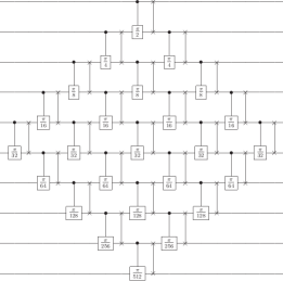
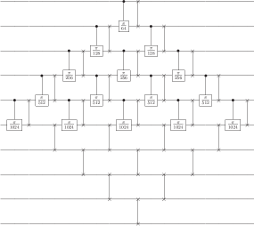
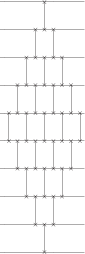
Abbildung 17: Equivalent circuit representations of the three $10$-qubit cp-swap modules needed for a $k\cdot 10$-qubit qft, when rotation angles less than $\pi/2^{10}$ are omitted (as described in the text): (a) cp-swap${}_{10}^{1}$ with no truncation so $F_{tr}=1$, (b) cp-swap${}_{10}^{2}$ with $F_{tr}=0.9999902$ , and (c) cp-swap${}_{10}^{j}$, which covers all $j\geq 3$ with fidelity $F_{tr}\geq 0.9999991$. These building blocks are compiled directly as effective $10$-qubit modules thus reducing the time to less than $60\%$ of the duration required for the decomposition into $2$-qubit modules.