Symmetry Breaking Study with Random Matrix Ensembles

Abstract

A random matrix model to describe the coupling of $m$-fold symmetry is constructed. The particular threefold case is used to analyze data on eigenfrequencies of elastomechanical vibration of an anisotropic quartz block. It is suggested that such experimental/theoretical study may supply a powerful means to discern intrinsic symmetry of physical systems.

The standard ensembles of Random Matrix Theory (RMT) Meht have had wide application in the description of the statistical properties of eigenvalues and eigenfunctions of complex many-body systems. Other ensembles have also been introduced Dyson , in order to cover situations that depart from universality classes of RMT. One such class of ensembles is the so-called Deformed Gaussian Orthogonal Ensemble (DGOE) Pato1 ; Pato2 ; Pato3 ; Carneiro:1991 that proved to be particularly useful when one wants to study the breaking of a discrete symmetry in a many-body system such as the atomic nucleus.

In fact, the use of spectral statistics as a probe of symmetries in physical systems has been a subject of intensive experimental and theoretical investigation following the pioneering work of Bohigas, Giannoni and Schmit Bohigas which showed that the quantal behaviour of classically chaotic systems exhibits the predictions supplied by the RMT. Examples of symmetry breaking in physical systems that have been studied include nuclei Mitch0 ; Mitch , atoms Simons ; Welch and mesoscopic devices such as quantum dots Alhassid .

In the case of nuclei, the Mitchell group at the Triangle Universities Nuclear Laboratory Mitch0 ; Mitch , studied the effect of isospin symmetry breaking, in odd-odd nuclei such as ${}^{26}Al$. They detected the breakdown of this important symmetry by the applications of two statistics: the short-range, nearest neighbor level spacing distribution (NND) and the long range Dyson’s $\Delta$-statistics Mitch0 ; Mitch . These results were well described by a DGOE in which a pair of diagonal blocks is coupled. The strength of the coupling needed to account for the symmetry breaking can be traced to the average matrix element of the Coulomb interaction responsible for this discrete symmetry breaking Pato2 ; Guhr . The justification for the use of block matrices to describe the statistics of a superposition of $R$ spectra with different values of the conserved quatum number can be traced to Refs. Meht ; NovaR . In the case of non-interacting spectra, i.e. if the quantum number is exactly conserved, the answer is a superposition of the $R$ spectra. Since the level repulsion is present in each one of the $R$ spectra, their superposition does not show this feature. Thus, we can say that for each spectra of states of a given value of the quantum number, one attaches a random matrix (GOE). For $R$ spectra each of which has a given value of the conserved quantum number, one would have an $R\times R$ block diagonal matrix. Each block matrix will have a dimension dictated by the number state of that spectra. If the quantum number is not conserved then the $R\times R$ block matrix acquires non-diagonal matrices that measure the degree of the breaking of the associated symmetry. This idea was employed by Guhr and Weidenmüller Guhr and Hussein and Pato Pato1 to discuss isopin violation in the nucleus ²⁶Al. In reference Pato1 , the random block matrix model was called the Deformed Gaussian Orthogonal Ensemble (DGOE).

In order to study transitions amongst universal classes of ensembles such as order-chaos (Poisson$\rightarrow$GOE), symmetry violation transitions (2GOE$\rightarrow$1GOE), experiments on physical systems are more complicated due to the difficulty of tuning the interaction (except, e.g. in highly excited atoms where the application of a magnetic field allows the study of GOE-GUE transitions). To simulate the microscopic physical systems, one relies on analog computers such as microwave cavities, pioneered by A. Richter and collaborators achim1 and acoustic resonators of Ellegaard and collaboratorsElleg0 ; Elleg ; Elleg2 . It is worth mentioning at this point that the first to draw attention to the applicability of RMT to accoustic waves in physical system was Weaver Weaver .

In the experiment of Ellegaard et al. Elleg what was measured were eigenfrequencies of the elastomechanical vibrations of an anisotropic crystal block with a D3 point-group symmetry. The rectangular crystal block employed by Ellegard was so prepared as to have only a two-fold flip symmetry retained. Then, to all effects, the quartz specimen resembles a system of two three-dimensional Sinai billiards. The statistical treatment of the eigenfrequencies of such a block would follow that of the superposition of two uncoupled GOE’s.

Then, by removing octants of progressively larger radius from a corner of the crystal block this remnant two-fold symmetry was gradually broken. The spectral statistics show a transition towards fully a chaotic system as the octant radius increases. What was then seen was that the measured NND is compatible with a two block DGOE description but the $\Delta$-statistics was discrepant. This discrepancy was attributed to pseudo integrable behavior and this explanation was later implemented with the result that the long-range behavior was fitted at the cost, however, of loosing the previous agreement shown by the NNDAbul .

Here we reanalyse this experiment following the simpler idea of extending the DGOE matrix model Pato3 to consider the coupling of three instead of two GOE’s Carneiro:1991 . We show that within this extension both, the short- and the long-range statistics, are reasonably fitted suggesting that the assumption of the reduction of the complex symmetries of anisotropic quartz block may not be correct. Our findings have the potential of supplying very precise means of testing details of symmetry breaking in pysical systems.

To define the ensembles of random matrices we are going to work with, we recall the construction based on the Maximum Entropy Principle Pato1 , that leads to a random Hamiltonian which can be cast into the form

$$H=H_{0}+\lambda H_{1},$$ (1)

where the block diagonal $H_{0}$ is a matrix made of $m$ uncoupled GOE blocks and $\lambda$ ($0\leq\lambda\leq 1)$ is the parameter that controls the coupling among the blocks represented by the $H_{1}$ off-diagonal blocks. For $\lambda=1,$ the $H_{1}$ part completes the $H_{0}$ part and $H=H^{GOE}.$

These two matrices $H_{0}$ and $H_{1}$ are better expressed introducing the following $m$ projection operators

$$P_{i}=\sum\limits_{j\in I_{i}}\mid j><j\mid,$$ (2)

where $I_{i}$ defines the domain of variation of the row and column indexes associated with $i$th diagonal block of size $M_{i}.$ Since we are specifically interested in the transition from a set of $m$ uncoupled GOE’s to a single GOE, we use the above projectors to generalize our previous model Pato1 ; Pato2 by writing

$$H_{0}=\sum\limits_{i=1}^{m}P_{i}H^{GOE}P_{i}$$ (3)

and

$$H_{1}=\sum\limits_{i=1}^{m}P_{i}H^{GOE}Q_{i}$$ (4)

where $Q_{i}=1-P_{i}.$ It is easily verified that $H=H^{GOE}$ for $\lambda=1.$

The joint probability distribution of matrix elements can be put in the form Pato1 ; Alberto

$$P(H,\alpha,\beta)=Z_{N}^{-1}\exp\left(-\alpha trH^{2}-\beta trH_{1}^{2}\right)$$ (5)

with the parameter $\lambda$ being given in terms of $\alpha$ and $\beta$ by

$$\lambda=(1+\beta/\alpha)^{-1/2}.$$ (6)

Statistical measures of the completely uncoupled $m$ blocks have been derived. They show that level repulsion disappears which can be understood since eigenvalues from different blocks behave independently. In fact, as $m$ increases the Poisson statistics are gradually approached. In the interpolating situation of partial coupling, some approximate analytical results have been derived. In Ref. Alberto , for instance, it has been found that the density $\rho(E)$ for arbitrary $\lambda$ and $m$ is given by

$$\rho(E)=\sum\limits_{i=1}^{m}\frac{M_{i}}{N}\rho_{i}(E)$$ (7)

where

$$\rho_{i}(E)=\left\{\begin{array}[]{rl}\frac{2}{\pi a_{i}^{2}}\sqrt{{a_{i}^{2}-E^{2}}},&\mid E\mid\leq a\\ 0,&\mid E\mid>a\end{array}\right.$$ (8)

is Wigner’s semi-circle law with $a=\sqrt{N/\alpha}$ and

$$a_{i}=a^{2}\left[\frac{M_{i}}{N}+\lambda^{2}\left(1-\frac{M_{i}}{N}\right)\right].$$ (9)

The transition parameter utilized in the following is defined as Pandey:1995

$$\Lambda=\lambda^{2}\rho(0)^{2}=\lambda^{2}\frac{N^{2}}{\pi a/2}.$$ (10)

Eq. (5) can be used to calculate exactly analytically the NND for $2\times 2$ and $3\times 3$ matrices Carneiro:1991 . For the $2\times 2$ case the DGOE, Eq. (5), gives

$$P_{2\times 2}(s,\Lambda)=s\sqrt{\frac{\pi}{8\Lambda}}I_{0}(\frac{s^{2}}{16\Lambda})\exp\left(-\frac{s^{2}}{16\Lambda}\right),$$ (11)

where $I_{0}$ is the modified Bessel function, whose asymptotic form is

$$I_{0}(x)\rightarrow\frac{e^{x}}{\sqrt{2\pi x}}.$$ (12)

Thus, $P_{2\times 2}(s,0)=1$, and there is no level repulsion for $\Lambda\rightarrow 0$. In the opposite limit, $\Lambda\rightarrow\infty$, $I_{0}(x)\approx 1-x^{2}/4$ and one obtains

$$P_{2\times 2}(s,\Lambda\gg 1)\approx s\sqrt{\frac{\pi}{8\Lambda}}e^{-s^{2}/16\Lambda}.$$ (13)

For higher dimensions Eq. (5) can only be used for numerical simulations, however, using appropriate perturbative methods Leitner Leitner was able to find a formula for the NND. He started basically with the formula for the nearest neigbhour spacing distribution for the superposition of $m$ GOE’s block matrices Meht

$$P_{m}(s)=\frac{d^{2}}{ds^{2}}E_{m}(s)$$ (14)

where, for the case of all block marices having the same dimension one has

$$E_{m}(s)=\left(E_{1}(\frac{s}{m})\right)^{m},$$ (15)

$$E_{1}(x)=\int_{x}^{\infty}(1-F(t))\,dt,$$ (16)

$$F(t)=\int_{0}^{t}P_{1}(z)\,dz.$$ (17)

In the above $P_{1}(z)$ is the normalized nearest neighbour spacing distribution of one block matrix. It is easy to find for $P_{m}(s)$, the following

$$P_{m}(s) = \frac{1}{m}\left[\left(E_{1}(s/m)\right)^{m-1}P_{1}(s/m)+(m-1)(E_{1}(s/m))^{m-2}(1-F(s/m))^{2}\right]$$ (18)

$$\equiv P^{(1)}_{m}(s)+P_{m}^{(2)}(s)$$ (19)

If all the block matrices belong to the GOE, then one can use the Wigner form for $P_{1}(z)$

$$P_{1}(z)=\frac{\pi}{2}ze^{-\frac{\pi}{4}z^{2}}\approx\frac{\pi}{2}z,$$ (20)

thus

$$F_{1}(z)=1-e^{-\frac{\pi}{4}z^{2}}\approx\frac{\pi}{4}z^{2},$$ (21)

$$E_{1}(z)=erfc\left(\frac{\sqrt{\pi}}{2}z\right)\approx 1-z.$$ (22)

where the large-$z$ limits of Eqs. (20)-(22) are also indicated above. It is now clear that the above expression for $P_{m}(s)$, (18) and (19), contains a term $P_{m}^{(1)}(s)$ with level repulsion, indicating short-range correlation among levels pertaining to the same block matrix and a second term $P_{m}^{(2)}(s)$ with no level repulsion, implying short-range correlation among NND levels pertaining to different blocks. Notice that for very small spacing, $P_{m}(s)$ behaves as

$$P_{m}(s)\approx\frac{\pi}{2m^{2}}s+\frac{m-1}{m}$$ (23)

for $m=1$, we get the usual $P_{1}(0)=0$, while for $m>1$, we get $P_{m}(0)=(m-1)/m$. To account for symmetry breaking, Leitner Leitner considered the mixing between levels pertaining to nearest neigbhour block matrices. This amount to constrain the mixing to be of the form given by Eq. (11) for the $2\times 2$ DGOE, thus, he found

$$P_{m}(s,\Lambda)=P_{m}^{(1)}(s)+P_{2\times 2}(s,\Lambda)P_{m}^{(2)}(s).$$ (24)

Though $P_{m}(s)$ is normalized, $P_{m}(s,\Lambda)$ is not. Accordingly one supplies coefficients $c_{N}$ and $c_{D}$, such that

$$P_{m}(s,\Lambda,c_{N},c_{D})\equiv c_{N}P_{m}(c_{D}s,\Lambda)$$ (25)

is normalized to unity. Similarly, $<s>$ should be unity too. Eq. (24) can certainly be generalized to consider the effect of mixing of levels pertaining to next to nearest neighbour blocks, and accordingly, $P_{3\times 3}(s,\Lambda)$, given in Ref. Carneiro:1991 would be used in Eq. (24) instead of $P_{2\times 2}(s,\Lambda)$. In the following, however, we use Eqs. (24), (25) as Leitner did Leitner .

In Ref. Leitner , Leitner also obtained approximate expression for the spectral rigidity $\Delta_{3}(L)$ using results derived by French et al. French . Leitner’s approximation to $\Delta_{3}$ is equal to the GOE spectral rigidity plus perturbative terms, that is

$$\Delta_{3}^{(m)}(L;\Lambda) \approx \Delta_{3}(L;\infty)+\frac{m-1}{\pi^{2}}\left[\left(\frac{1}{2}-\frac{2}{\epsilon^{2}L^{2}}-\frac{1}{2\epsilon^{4}L^{4}}\right)\right.$$ (26)

$$\times\ln(1+\epsilon^{2}L^{2})+\frac{4}{\epsilon L}\tan^{-1}(\epsilon L)+\left.\frac{1}{2\epsilon^{2}L^{2}}-\frac{9}{4}\right],$$

where

$$\epsilon = \frac{\pi}{2(\tau+\pi^{2}\Lambda)}$$ (27)

For the cut off parameter we use the value Abul-Magd:2004 $\tau=c_{m}e^{\pi/8-\gamma-1},$ where $c_{m}=m^{m/(m-1)}$ and $\gamma\approx 0.5772$ is Euler’s constant. This choice guarantees that when the symmetry is not broken, $\Lambda=0$, $\Delta_{3}^{(m)}(L,0)=m\Delta_{3}(L/m,\infty)$. In Ref. Leitner:1997 , Leitner fitted Eq. (25) for $m$=2 to the NND from Ref. Elleg , however, he did not fit the spectral rigidity. It is often the case that there are some missing levels in the statistical sample analysed. Such a situation was addressed recently by Bohigas and Pato ML who have shown that if $g$ fraction of the levels or eigenfrequencies is missing, the $\Delta_{3}(L)$ becomes

$$\Delta_{3}^{g}(L)=g\frac{L}{15}+(1-g)^{2}\Delta_{3}\left(\frac{L}{1-g}\right).$$ (28)

The presence of the linear term, even if small, could explain the large $L$ behavior of the measured $\Delta_{3}(L)$. We call this effect the Missing Level (ML) effect. Another possible deviation of $\Delta_{3}$ from Eq. (26) could arise from the presence of pseudo-integrable effect (PI) Abul ; bis2 . This also modifies $\Delta_{3}$ by adding a Poisson term just like Eq. (28).

We now apply our model to analyse the eigenfrequency data of the elastomechanical vibrations of an anisotropic quartz block used in Elleg . In this reference in order to break the flip symmetry of the crystal block gradually they removed an octant of a sphere of varying size at one of the corners. The rectangular quartz block has the dimensions $14\times 25\times 4\,mm^{3}$. The radii of the spheres containing the octants are $r=0.0,0.5,0.8,1.1,1.4$ and $1.7\,mm$ representing figures $(a)-(f)$. Figs. $1x$ and $2x$ of Ref. Elleg correspond to the octant $r\gg 1.7$. They found 1424, 1414, 1424, 1414, 1424 and 1419 frequency eigenmodes, respectively. The histograms and circles in the two figures of Ref. Elleg represent the short-range nearest-neighbor distributions $P(s)$ (Fig. 1) and the long range $\Delta_{3}(L)$ statistics (Fig. 2).

The results of our analysis are shown in the two figures. In Fig. 1, the sequence of six measured NNDs were fitted for $m=2$ and $m=3.$ It can be seen that the DGOE model with three coupled GOE’s give a comparable and in some cases even better fit than the $m=2$ one. Figure 1a in fact shows a rather sharp peak in our calculated $P(s)$ for $m=3$, $P_{3}(s,0.0056)$. We consider this a failure of our formula (25) for the uncut crystal. In fact, a more appropriate description of the uncut crystal is to take $\Lambda=0$, namely a superposition of 3 uncoupled GOE’s, which works almost as good as the 2 uncoupled GOE’s description. The other parts of figure 1, $(b)-(x)$ seem to show the same insensitivity of $P_{m}(s,\Lambda)$ to $m$; the number of matrix blocks used in DGOE description. It is this insensitivity of the short-range nearest neighbour level correlation, measured by the spacing distribution, to the assumed symmetry inherent in the uncut crystal (and thus the number uncoupled GOE’s employed to describe it) that forces us to examine the long-range level correlation, namely spectral rigidity, “measured” by Dyson’s $\Delta_{3}$ statistics.

In Fig. 2. the $\Delta$-statistic was fitted with equation (26). It is clear from the figure that a good fit to the data of Ref. Elleg is obtained with $m=3$ for the values of $\Lambda$ given in table 1. This is to be contrasted with the case of $m=2$ which, according to Eq. (26) results in $\Delta_{3}^{(2)}(L,\Lambda)$ that is always below the one with $\Lambda=0$, $\Delta_{3}^{(2)}(L,0)$, which itself is always below the data points of Ref. Elleg . For this reason, only the $\Delta_{3}^{(2)}(L,0)$ is shown in the figure. It should be noted that the $\Delta$-statistics of the uncut crystal, Fig. 2a is very well described by that of 3 uncoupled GOE’s, namely $\Delta_{3}^{(3)}(L)=3\Delta_{3}^{(1)}(L/3)$ which is always larger than the above mentioned $\Delta_{3}^{(2)}(L)=2\Delta_{3}^{(1)}(L/2)$. The most conspicuous exception is Fig. 2b which corresponds to $r=0.5\,mm$ and where $1414$ frequency eigenvalues were found. We consider this a potential ML case and take for $\Delta_{3}$, the expression given in Eq. (28) and use it in Eq. (26). We find perfect fit to the data, if $g$ is taken to be $6\%$, namely only $94\%$ of the eigenfrequencies were in fact taken into account in the statistical analysis. In contrast, if 2GOE is used we still do not get very good agreement even if 18% of the levels are taken to be missing, as shown in Fig 3. There is, threfore, room to account much better for all cases (Fig. $2a$, $2c$, $\ldots$ ) by appropiately choosing the correponding value of $g$.

Table 1: Values of $\Lambda$ obtained by fitting Eqs. (25) and (26) respectively to the experimental NNDs and spectral rigidities from Ref. Elleg .

	$P(s)$			$\Delta_{3}(L)$
Data Set	Ref. Leitner:1997	Eq. (25) $m$=2	Eq. (25) $m$=3	Eq. (26) $m$=3
(a)	0.0013	0.0030	0.0067	0.0056
(b)	0.0054	0.0063	0.0098	0.0016
(c)	0.0096	0.010	0.017	0.0017
(d)	0.0313	0.032	0.064	0.027
(e)	0.0720	0.070	0.13	0.050
(f)	0.113	0.12	0.30	0.16
(x)	0.138	0.13	0.34	2.4

In conclusion, a random matrix model to describe the coupling of $m$-fold symmetry is constructed. The particular threefold case is used to analyse data on eigenfrequencies of elastomechanical vibration of a anisotropic quartz block. By properly taking into account the ML effect we have shown that the quartz block could very well be described by 3 uncoupled GOE’s , which are gradually coupled by the breaking of the three-fold symmetry (through the gradual removal of octants of increasing sizes), till a 1GOE situation is attained. This, therefore, indicates that the unperturbed quartz block may posses another symmetry, besides the flip one. We have also verified that if a 2GOE description is used, namely, $m=2$ , then an account of the large-$L$ behaviour of $\Delta_{3}$ can also be obtained if a much larger number of levels were missing in the sample. In our particular case of Fig. 2b, we obtained $g=0.18$. This is 3 times larger than the ML needed in the 3GOE description. We consider the large value of $g$ needed in the 2GOE description, much too large to conform to the reported data in Ref Elleg . A preliminary version of the formal aspect of this work has appeared in last .

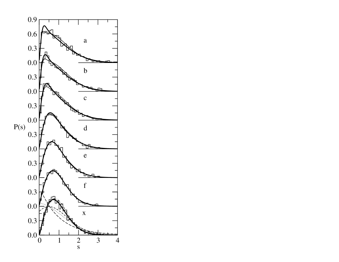
Figure 1: Nearest Neighbour Distributions. Histograms show data (a)-(x) from Ref. Elleg . Thin and thick solid lines show fits to the data carried out using Eq. (25) with m=2 and m=3 respectively. In graph (x) the long-dashed line is the Poisson distribution, the dot-dashed line is the Wigner distribution and the dashed and dotted lines are the respective distributions for superpositions of 2 and 3 uncoupled GOEs. See Table I for the values of $\Lambda$ obtained from the fits and the text for details.

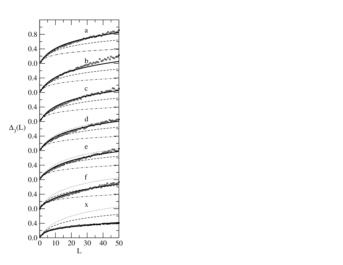
Figure 2: Spectral Rigidities. Circles show data (a)-(x) from Ref. Elleg . Thick solid lines show fits to the data carried out using Eq. (25) with m=3. The dot-dashed line is the GOE spectral rigidity and the dashed and dotted lines are the respective rigidities for superpositions of 2 and 3 uncoupled GOEs. See Table I for the values of $\Lambda$ obtained from the fits.

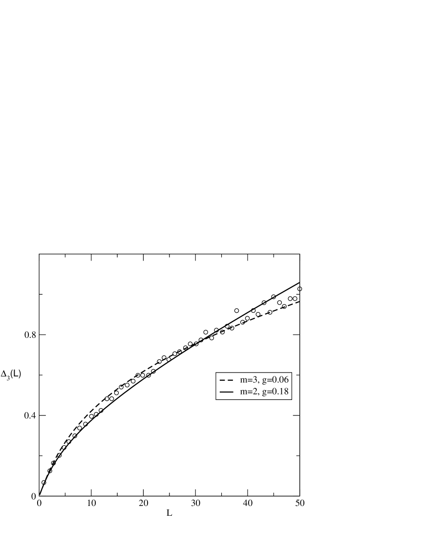
Figure 3: The Missing Level Effect: The full curve is the 2GOE $\Delta_{3}$ for case 2b with 18% of the levels missing, while the dashed curve corresponds to 3GOE with only 6% of the levels missing. The data points (open circles) represent fig. 2b. See text for details.

References

- (1) M.L. Mehta, Random Matrices 2nd Edition (Academic Press, Boston, 1991); T.A. Brody et al., Rev. Mod. Phys. 53, 385 (1981); T. Guhr, A. Müller-Groeling and A. Weidenmüller, Phys. Rep. 299, 189 (1998).
- (2) F.J. Dyson, J. Math. Phys. 3, 1191 (1962).
- (3) M. S. Hussein, and M.P. Pato, Phys. Rev. Lett. 70, 1089 (1993).
- (4) M. S. Hussein, and M.P. Pato, Phys. Rev. C 47, 2401 (1993).
- (5) M. S. Hussein, and M.P. Pato, Phys. Rev. Lett. 80, 1003 (1998).
- (6) C. E. Carneiro, M. S. Hussein e M. P. Pato, in H. A. Cerdeira, R. Ramaswamy, M. C. Gutzwiller and G. Casati (eds.) Quantum Chaos, p. 190 (World Scientific, Singapore) (1991).
- (7) O. Bohigas, M. J. Giannoni and C. Schmit, Phys. Rev. Lett. 52, 1 (1984). See also O. Bohigas and M. J. Giannoni, in Mathematical and Computational Methods in Nuclear Physics, edited by J. S. DeHesa, J. M. Gomez and A. Polls, Lecture Notes in Physics Vol. 209 (Springer-Verlag, New York, 1984).
- (8) G. E. Mitchell, E. G. Bilpuch, P. M. Endt, and F. J. Shriner, Phys. Rev. Lett. 61, 1473 (1988).
- (9) A.A. Adams, G.E. Mitchell, and J.F. Shriner, Jr., Phys. Lett. B 422, 13 (1998).
- (10) B. D. Simons, A. Hashimoto, M. Courtney, D. Kleppner and B. L. Altshuler, Phys. Rev. Lett. 71, 2899 (1993).
- (11) G. R. Welch, M. M. Kash, C-h Iu, L. Hsu and D. Kleppner, Phys. Rev. Lett. 62, 893 ( 1989).
- (12) See, e.g. Y. Alhassid, Rev. Mod. Phys. 72, 895 (2000) and references therein.
- (13) T. Guhr and, H.A. Weidenmüller. Ann. Phys. (NY), 199, 412 (1990).
- (14) N. Resenzweig and C. E. Porter, Phys. Rev. 120, 1698 (1960).
- (15) H.-D. Graf, H. L. Harney, H. Lengeler, C. H. Lewnkopf, C. Rangacharyulu, A. Richter, P. Schardt and H. A. Weidenmuller, Phys. Rev. Lett. 69, 1296(1992); H. Alt, H. -D. Graf, H. L. Harney, R. Hofferbert, H. Lengeler, A. Richter, P. Schardt and H. A. Weidenmuller, Phys. Rev. Lett. 74, 62 (1995); H. Alt, C. Dembowski, H. -D. Graf, R. Hofferbert, H. Rehfeld, A. Richter, R. Schuhmann and Weiland, Phys. Rev. Lett. 79, 1029 (1997); H. Alt, C. I. Brabosa, H. -D. Graf, T. Guhr, H. L. Harney, R. Hofferbert, H. Rehfeld and A. Richter, Phys. Rev. Lett. 81, 4847 (1998); C. Dembowski, H. -D. Graf, A. Heine, R. Hofferbert, H. Rehfeld and A. Richter, Phys. Rev. Lett. 84, 867 (2000); C. Dembowski, H. -D. Graf. H. L. Harney, A. Heine, W. D. Heiss, H. Rehfeld and A. Richter, Phys. Rev. Lett. 86, 787 (2001); C. Dembowski, H. -D. Graf, A. Heine, T. Hesse, H. Rehfeld and A. Richter, Phys. Rev. Lett. 86, 3284 (2001); C. Dembowski, B. Dietz, H. -D. Graf, A. Heine, T. Papenbrock, A. Richter and C. Richter, Phys. Rev. Lett. 89, 064101-1 (2002); C. Dembowski, B. Dietz, A. Heine, F. Leyvraz, M. Miski-Oglu, A. Richter and T. H. Seligman, Phys. Rev. Lett. 90, 014102-1 (2003); C. Dembowski, B. Dietz, H. -D. Graf, H. L. Harney, A. Heine, W. D. Heiss and A. Richter, Phys. Rev. Lett. 90, 034101-1 (2003); C. Dembowski, B. Dietz, T. Friedrich, H. -D. Graf, A. Heine, C. Mejia-Monasterio, M. Miski-Oglu, A. Richter and T. H. Seligman, Phys. Rev. Lett. 93, 134102-1 (2004); B. Dietz, T. Guhr, H. L. Harney and A. Richter, Phys. Rev. Lett. 96, 254101 (2006); E. Bogomolny, B. Dietz, T. Friedrich, M. Miski-Oglu, A. Richter, F. Schafer and C. Schmit, Phys. Rev. Lett. 97, 254102 (2006); B. Dietz, T. Friedrich, H. L. Harney, M. Miski-Oglu, A. Richter, F. Schafer and H. A. Weidenmuller, Phys. Rev. Lett. 98, 074103 (2007).
- (16) C. Ellegaard, T. Guhr, K. Lindemann, H. Q. Lorensen, J. Nygard and M. Oxborrow, Phys. Rev. Lett. 75, 1546 (1995).
- (17) C. Ellegaard, T. Guhr, K. Lindemann, J. Nygard and M. Oxborrow, Phys. Rev. Lett. 77, 4918 (1996).
- (18) P. Bertelsen, C. Ellegaard, T. Guhr, M. Oxborrow and K. Schaadt, Phys. Rev.Lett. 83, 2171 (1999).
- (19) R. L. Weaver, J. Acoustic. Soc. Am. 85, 1005 (1989).
- (20) A. Abd El-Hady, A. Y. Abul-Magd, and M. H. Simbel, J. Phys. A 35, 2361 (2002).
- (21) A. C. Bertuola, J. X. de Carvalho, M. S. Hussein, M. P. Pato, and A. J. Sargeant, Phys. Rev. E 71, 036117 (2005).
- (22) A. Pandey, Chaos, Solitons and Fractals 5 (1995) 1275.
- (23) D. M. Leitner, Phys. Rev. E 48, 2536 (1993).
- (24) J. B. French, V. K. B. Kota, A. Pandey and S. Tomsovic, Ann. Phys. (NY) 181, 198 (1988).
- (25) A.Y. Abul-Magd and M.H. Simbel, Phys. Rev. E 70 (2004) 046218.
- (26) D.M. Leitner, Phys. Rev. E 56 (1997) 4890.
- (27) O. Bohigas and M. P. Pato, Phys. Lett. B, 595, 171 (2004).
- (28) D. Biswas and S. R. Jain, Phys. Rev. A 42, 3170 (1990).
- (29) M. S. Hussein, J. X. de Carvalho, M. P. Pato and A. J. Sargeant, Few-Body Systems, 38, 209 (2006).