On the Korteweg-de Vries approximation
for uneven bottoms

Abstract

In this paper we focus on the water waves problem for uneven bottoms on a two-dimensionnal domain. Starting from the symmetric Boussinesq systems derived in [Chazel, Influence of bottom topography on long water waves, 2007], we recover the uncoupled Korteweg-de Vries (KdV) approximation justified in [Schneider-Wayne, The long-wave limit for the water-wave problem. I. The case of zero surface tension, 2002] for flat bottoms, and in [Iguchi, A long wave approximation for capillary-gravity waves and an effect of the bottom, 2007] in the context of bottoms tending to zero at infinity at a substantial rate. The goal of this paper is to investigate the validity of this approximation for more general bathymetries. We exhibit two kinds of topography for which this approximation diverges from the Boussinesq solutions. A topographically modified KdV approximation is then proposed to deal with such bathymetries, where topography-dependent terms are added to the solutions of the KdV equations. Finally, all the models involved are numerically computed and compared.

Introduction

The water waves problem consists in describing the evolution of the free surface and velocity field of a layer of ideal, incompressible and irrotationnal fluid under the only influence of gravity. The governing equations - also called free surface Euler equations - are fully non-linear and non-strictly hyperbolic, and their direct study and computation remains a real obstacle. Many authors such as Nalimov ([44], 1974), Yoshihara ([57], 1982), Craig ([18], 1985), Wu ([55], 1997 and [56], 1999), Ambrose-Masmoudi ([4], 2005) and Lannes ([38], 2005 and [2], 2007) have successfully tackled the problem of well-posedness of these equations. Nevertheless, the numerical computation of these solutions remains a tough task, especially in 3-D - see the works of Grilli et al. ([25], 2001) and Fochesato-Dias ([23], 2001).
An alternative way to describe these solutions and their time behaviour is to look for approximations via the use of asymptotic models. Such models are usually derived formally from the water waves problem by introducing dimensionless parameters. Making some hypothesis on these parameters reduces the framework to more limited physical regimes but allows the construction of asymptotic models. In this work, we focus on the so-called long waves regime. In this regime, the ratios $\displaystyle\varepsilon=a/h_{0}$ and $\displaystyle\mu=h_{0}^{2}/\lambda^{2}$ where $\displaystyle a$ denotes the typical amplitude of the waves, $\displaystyle h_{0}$ the mean depth and $\displaystyle\lambda$ the typical wavelength, are small and of the same order. Many models can be found in the litterature corresponding to this regime. Among them, we can quote the works of Boussinesq ([14], 1871 and [15], 1872) who was the first to propose a model that take into account both nonlinear and dispersive effects, the unidirectional models such as the Korteweg-de Vries (KdV) equation ([36], 1895), the Kadomtsev-Petviashvili (KP) equation ([31], 1970) and the Benjamin-Bona-Mahony one ([5], 1972). These historical models have been considerably studied and generalized, and their justification has been investigated among others by Craig ([18], 1985), Schneider-Wayne ([50], 2000), Bona-Colin-Lannes ([12], 2005), Lannes-Saut ([40], 2006) for flat bottoms, and Iguchi ([26], 2006), Chazel ([16], 2007), Alvarez-Lannes ([2], 2007) for uneven bottoms.
If we focus more specifically on the KdV approximation, we emphasize that the investigation of this model on uneven bottoms is not recent : this subject has been tackled among others by Ostrovskii-Pelinovskii ([48], 1970), Kakutani ([32], 1971), Johnson ([28], 1973), Miles ([43], 1979) and Newell ([45], 1985). However, their approach is quite different compared to the one chosen here, as will be clarified later in this paper. The more recent articles of Iguchi ([26], 2006) and Chazel ([16], 2007) are somehow the starting point of the present work. In [26], Iguchi derived two different models : a coupled KdV system for relatively general bottom topographies, and a uncoupled KdV system for bathymetries decaying at a substantial rate at infinity. In [16], the author derived two classes of symmetric Boussinesq systems for two bottom topography scales, corresponding respectively to slightly and largely varying bottoms. The aim of this work is to recover the uncoupled KdV model - also justified by Schneider-Wayne [50] for flat bottoms - starting from any previous Boussinesq system proposed in [16] for slightly varying bottoms, to discuss its validity regarding the bottom topography, and to propose an alternative.

Formulation of the problem

In this paper, we work in two dimensions : $\displaystyle x$ corresponds to the horizontal coordinate and $\displaystyle y$ to the vertical one. We denote by $\displaystyle(t,x)\rightarrow\eta(t,x)$ and $\displaystyle x\rightarrow b(x)$ the parametrizations of the free surface and bottom, defined respectively over the surface $\displaystyle y=0$ and the mean depth $\displaystyle y=-h_{0}$ at the steady state. The time-dependant domain $\displaystyle\Omega_{t}$ of the fluid is thus taken of the form :

$$\Omega_{t}=\{(x,y),\,x\in\mathbb{R},\,-h_{0}+b(x)\leq y\leq\eta(t,x)\}\;\;.$$

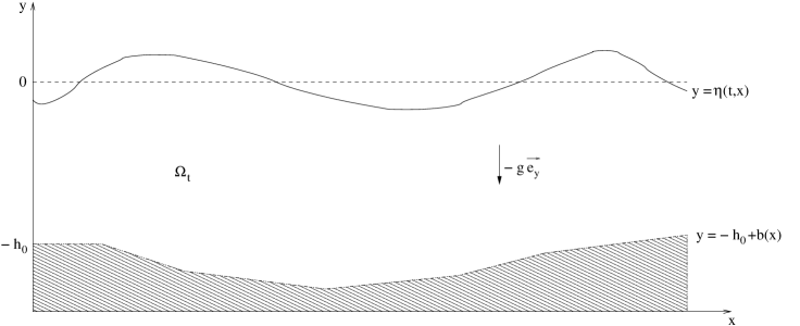
Figure 0.1: Representation of the fluid domain

For the sake of simplicity, we assume here that $\displaystyle b\in W^{k,\infty}(\mathbb{R}^{d})$, $\displaystyle k$ being as large as needed, where we recall that $\displaystyle W^{k,\infty}(\mathbb{R}^{d})=\{u\,/\,\partial_{x}^{m}u\in L^{\infty}(\mathbb{R}^{d}),0\leq m\leq k\}$. In order to avoid some special physical cases such as the presence of islands or beaches, we set a condition of minimal water depth : there exists a strictly positive constant $\displaystyle h_{min}$ such that

$$\eta(t,x)+h_{0}-b(x)\geq h_{min}\;\;,\;\;(t,x)\in\mathbb{R}\times\mathbb{R}\;\;.$$ (0.1)

We introduce the following dimensionless parameters :

$$\varepsilon=\frac{a}{h_{0}}\;\;,\;\;\mu=\frac{h_{0}^{2}}{\lambda^{2}}\;\;,\beta=\frac{\beta_{0}}{h_{0}}\;\;,$$

where $\displaystyle a$ denotes the typical amplitude of the waves, $\displaystyle h_{0}$ the mean depth, $\displaystyle\lambda$ the typical wavelength and $\displaystyle\beta_{0}$ the typical amplitude of the bottom topography. In the present long waves regime, one has $\displaystyle\varepsilon\ll 1$, $\displaystyle\mu\ll 1$ and $\displaystyle\varepsilon\approx\mu$, i.e. the Stokes number $\displaystyle S=\varepsilon/\mu$ is of order $\displaystyle O(1)$. Moreover, one has $\displaystyle\beta=B_{0}\varepsilon$ with $\displaystyle B_{0}=O(1)$ since we focus here on slightly varying bottoms, i.e. bathymetries of small amplitude. We do not make any mild-slope assumption on the spatial variations of the bottom, i.e. the bathymetry can vary rapidly. For the sake of simplicity, we take the Stokes number $\displaystyle S$ and the constant $\displaystyle B_{0}$ equal to one, which implies that we have $\displaystyle\mu=\beta=\varepsilon$. This choice only lightens the writings by suppressing the constants $\displaystyle S$ and $\displaystyle B_{0}$ from the equations, and has no influence on the following results.

In [16], the author justified a whole class of symmetric Boussinesq systems as being asymptotic models to the water waves problem for slightly varying bottoms in 2-D and 3-D, assuming the existence of the water waves solutions on a large time scale. This assumption has been recently proved by Alvarez-Lannes in [2], where the authors systematically justified the main asymptotics models used in coastal oceanography. The justification of these symmetric Boussinesq models is hence complete. All the details on the construction and justification of these models can be found in [16]; the expression of such symmetric systems in 1-D surface is as follows :

$$(\Sigma)\left\{\begin{array}[]{l}\vspace{0.5em}(1-\varepsilon a_{2}\partial_{x}^{2})\partial_{t}v+\partial_{x}\eta+\varepsilon\Big{[}\frac{1}{2}\eta\partial_{x}\eta+\frac{3}{2}v\partial_{x}v-\frac{1}{2}b\partial_{x}\eta+a_{1}\partial_{x}^{3}\eta\Big{]}=0\,,\\ (1-\varepsilon a_{4}\partial_{x}^{2})\partial_{t}\eta+\partial_{x}v+\varepsilon\Big{[}\frac{1}{2}\partial_{x}\left((\eta-b)v\right)+a_{3}\partial_{x}^{3}v\Big{]}=0\,,\end{array}\right.$$

with

$$\left\{\begin{array}[]{lll}\vspace{0.2em}a_{1}=-\lambda_{1}\frac{\theta^{2}-1}{2}&;&a_{2}=(\lambda_{1}-1)\frac{\theta^{2}-1}{2}\,,\\ a_{3}=\lambda_{2}(\frac{\theta^{2}}{2}-\frac{1}{6})&;&a_{4}=(1-\lambda_{2})(\frac{\theta^{2}}{2}-\frac{1}{6})\,,\end{array}\right.$$

and $\displaystyle(\theta,\lambda_{1},\lambda_{2})$ being chosen in $\displaystyle[0,1]\times\mathbb{R}^{2}$ such that $\displaystyle a_{1}=a_{3}$, $\displaystyle a_{2}\geq 0$, $\displaystyle a_{4}\geq 0$. The parameter $\displaystyle\theta$ determines the height $\displaystyle y=-1+\theta(\varepsilon\eta+1-\beta b)$ where the above velocity $\displaystyle v$ is taken. The parameters $\displaystyle\lambda_{1}$ and $\displaystyle\lambda_{2}$ are arbitrary parameters and have no physical meaning.
Several different set of values for $\displaystyle(\theta,\lambda,\mu)$ can be found such that the previous condition on $\displaystyle a_{1},a_{2},a_{3},a_{4}$ is verified, f.e. $\displaystyle\theta=\sqrt{2/3}$, $\displaystyle\lambda_{1}=\lambda_{2}=1/2$ which gives $\displaystyle a_{1}=a_{2}=a_{3}=a_{4}=1/12$. Throughout this paper, we denote by $\displaystyle(\Sigma)$ any of this symmetric system. This system is the starting point of our work.

Organization of the paper

The paper is organized as follows. In Section I, we recover the KdV approximation proposed by Schneider-Wayne [50] and Iguchi [26] as follows : we first diagonalize the system $\displaystyle(\Sigma)$ and then look for an approximation of the solution of the obtained coupled system. This approximation is searched under the form of a couple of waves $\displaystyle(U_{0},N_{0})$ moving in opposite directions, plus correcting terms $\displaystyle(U_{1},N_{1})$ that satisfy a sublinear growth condition. We show that $\displaystyle U_{0}$ and $\displaystyle N_{0}$ must satisfy a system of two uncoupled KdV equations, as shown by Iguchi in [26]. It is proved that this approximation is correct for sufficiently decaying initial data and topography.
In Section II, we discuss the validity of this approximation - which is equivalent to check the sublinear growth condition on the correctors $\displaystyle(U_{1},N_{1})$ - for non trivial bathymetries. An analysis of these terms allows us to weaken the decay assumptions on the initial data and the bathymetry. However, it appears clearly that some more general bathymetries can unvalidate the model, and two examples of bottoms are provided for which the approximation diverges : a bottom corresponding to a simple step and a slowly varying sinusoidal bottom. A topographically modified KdV approximation is then proposed by adding bottom-dependent correcting terms to the classical approximation.
In Section III, all these models - the Boussinesq one, the usual uncoupled KdV one and the topographically modified version - are numerically integrated and compared on the two bathymetries introduced in Section II. The numerical schemes are presented, and the results show that both the Boussinesq model and the alternative KdV approximation successfully reproduce the expected physical phenomenons.

1 The classical KdV approximation

In this section, we recover the usual uncoupled KdV approximation justified by Schneider and Wayne in [50] for flat botoms, and by Iguchi in [26] for slightly varying bottoms. To this end, we start with any of the symmetric Boussinesq system ($\displaystyle\Sigma$) derived in [16] and look for approximate solutions of the diagonalized version of ($\displaystyle\Sigma$) under the form of two waves moving in opposite directions. Each wave is shown to be slightly modulated in time with a dynamic governed by a KdV equation, while the correcting terms must solve an inhomogeneous transport equation. The sum of these two waves is proved to give an approximation of the solutions of ($\displaystyle\Sigma$) for sufficiently decaying initial data and topography.

1.1 Derivation of the approximation

Let us recall the expression of ($\displaystyle\Sigma$) :

$$(\Sigma)\left\{\begin{array}[]{l}\vspace{0.5em}(1-\varepsilon a_{2}\partial_{x}^{2})\partial_{t}v+\partial_{x}\eta+\varepsilon\Big{[}\frac{1}{2}\eta\partial_{x}\eta+\frac{3}{2}v\partial_{x}v-\frac{1}{2}b\partial_{x}\eta+a_{1}\partial_{x}^{3}\eta\Big{]}=0\,,\\ (1-\varepsilon a_{4}\partial_{x}^{2})\partial_{t}\eta+\partial_{x}v+\varepsilon\Big{[}\frac{1}{2}\partial_{x}\left((\eta-b)v\right)+a_{3}\partial_{x}^{3}v\Big{]}=0\,,\end{array}\right.$$

with $\displaystyle a_{2}\geq 0$ and $\displaystyle a_{4}\geq 0$. We point out that such a system is well posed for sufficiently smooth initial data and provides an approximation of the water waves problem of order $\displaystyle O(\varepsilon)$ for times of order $\displaystyle O(1/\varepsilon)$ (see [16] and [2] for further details).
In order to recover the KdV approximation, we first diagonalize $\displaystyle(\Sigma)$ by introducing the following unknowns :

$$U=v+\eta\;\;;\;\;N=v-\eta\;.$$

Plugging the relations $\displaystyle v=(U+N)/2$ and $\displaystyle\eta=(U-N)/2$ into $\displaystyle(\Sigma)$ yields the following coupled system $\displaystyle(\Gamma)$ in terms of $\displaystyle U$ and $\displaystyle N$ :

$$(\Gamma)\left\{\begin{array}[]{l}\vspace{0.5em}\partial_{t}U+\partial_{x}U+\varepsilon\left[\frac{1}{8}\partial_{x}(3U^{2}+N^{2}+2UN)-\frac{1}{2}b\partial_{x}U-\frac{1}{4}\partial_{x}b(U+N)\right.\\ \vspace{0.5em}\hskip 70.0001pt\left.-\frac{a_{2}}{2}\partial_{x}^{2}\partial_{t}(U+N)-\frac{a_{4}}{2}\partial_{x}^{2}\partial_{t}(U-N)+a_{1}\partial_{x}^{3}U\right]=0\,,\\ \vspace{0.5em}\partial_{t}N-\partial_{x}N+\varepsilon\left[\frac{1}{8}\partial_{x}(U^{2}+3N^{2}+2UN)+\frac{1}{2}b\partial_{x}N+\frac{1}{4}\partial_{x}b(U+N)\right.\\ \hskip 70.0001pt\left.-\frac{a_{2}}{2}\partial_{x}^{2}\partial_{t}(U+N)+\frac{a_{4}}{2}\partial_{x}^{2}\partial_{t}(U-N)-a_{1}\partial_{x}^{3}N\right]=0\,.\end{array}\right.$$

At this step, we choose to look for an approximate solution $\displaystyle(U_{app},N_{app})$ of $\displaystyle(\Gamma)$ of the form :

$$\displaystyle\left\{\begin{array}[]{l}\vspace{1em}U_{app}(t,x)=U_{0}(T,x-t)+\varepsilon U_{1}(T,t,x)\;,\\ N_{app}(t,x)=N_{0}(T,x+t)+\varepsilon N_{1}(T,t,x)\;,\end{array}\right.$$ (1.3)

where $\displaystyle T$ is the slow time variable $\displaystyle T=\varepsilon t$. The choice of variables $\displaystyle x-t$ for $\displaystyle U_{0}$ and $\displaystyle x+t$ for $\displaystyle N_{0}$ emphasizes that we look for solutions which - at first order - propagate at speed one, to the right for $\displaystyle U$ and to the left for $\displaystyle N$ : this comes from the first order equations on $\displaystyle U$ and $\displaystyle N$ which are respectively $\displaystyle(\partial_{t}+\partial_{x})U=0$ and $\displaystyle(\partial_{t}-\partial_{x})N=0$.
The use of two different time scales is useful in capturing both the short time evolution of the wave and the nonlinear and dispersive dynamics which occur for larger time scales.
We complement this ansatz with two initial conditions on $\displaystyle(U_{app},N_{app})$ and a classical sublinear growth condition on the correctors $\displaystyle(U_{1},N_{1})$ :

$$U_{app\,|_{t=0}}=U_{|_{t=0}}\;\;,\;\;N_{app\,|_{t=0}}=N_{|_{t=0}}\;,$$

and for all $\displaystyle T_{0}\geq 0$

$$\displaystyle\left\{\begin{array}[]{l}\vspace{1em}\lim_{t\rightarrow+\infty}\frac{1}{t}\,\left|\,U_{1}(.\,,t,.)\right|_{L^{\infty}([0,T_{0}];L^{2}(\mathbb{R}))}=0\;,\\ \lim_{t\rightarrow+\infty}\frac{1}{t}\,|\,N_{1}(.\,,t,.)|_{L^{\infty}([0,T_{0}];L^{2}(\mathbb{R}))}=0\;.\end{array}\right.$$ (1.6)

Such a condition on the correctors is quite usual in multiscales expansions and has been first introduced in the context of nonlinear geometric optics by Joly, Métivier and Rauch in [30]. It forces the correctors $\displaystyle\varepsilon U_{1}$ and $\displaystyle\varepsilon N_{1}$ to be small on the large time scale associated to the KdV dynamics ; namely, it ensures that $\displaystyle\varepsilon U_{1}=o(1)$ and $\displaystyle\varepsilon N_{1}=o(1)$ in $\displaystyle L^{\infty}([0,\frac{T_{0}}{\varepsilon}];L^{2}(\mathbb{R}))$.

Plugging this ansatz into $\displaystyle(\Gamma)$ and neglecting the terms of order $\displaystyle O(\varepsilon)$ yields the following system :

$$\left\{\begin{array}[]{l}\vspace{0.5em}(\partial_{t}+\partial_{x})U_{1}=f(T,x-t)-\frac{1}{8}\partial_{x}N_{0}^{2}-\frac{1}{4}\partial_{x}(U_{0}N_{0})+\frac{1}{2}b\partial_{x}U_{0}+\frac{1}{4}U_{0}\partial_{x}b\\ \hskip 70.0001pt+\frac{1}{4}N_{0}\partial_{x}b+\frac{a_{2}-a_{4}}{2}\,\partial_{x}^{3}N_{0}\;,\\ (\partial_{t}-\partial_{x})N_{1}=g(T,x+t)-\frac{1}{8}\partial_{x}U_{0}^{2}-\frac{1}{4}\partial_{x}(U_{0}N_{0})-\frac{1}{2}b\partial_{x}N_{0}-\frac{1}{4}U_{0}\partial_{x}b\\ \hskip 70.0001pt-\frac{1}{4}N_{0}\partial_{x}b-\frac{a_{2}-a_{4}}{2}\,\partial_{x}^{3}U_{0}\;,\end{array}\right.$$ (1.7)

$$\mbox{where}\;\;\left\{\begin{array}[]{l}\vspace{0.5em}f(T,x-t)=-\partial_{T}U_{0}-\frac{3}{8}\partial_{x}U_{0}^{2}-(a_{1}+\frac{a_{2}+a_{4}}{2})\,\partial_{x}^{3}U_{0}\;,\\ g(T,x+t)=-\partial_{T}N_{0}-\frac{3}{8}\partial_{x}N_{0}^{2}+(a_{1}+\frac{a_{2}+a_{4}}{2})\,\partial_{x}^{3}N_{0}\;.\end{array}\right.$$ (1.8)

N.B. : For the sake of simplicity, we have kept here the notations $\displaystyle\partial_{x}$ on $\displaystyle U_{0}$ and $\displaystyle N_{0}$ while we should have written rigorously $\displaystyle\partial_{X_{-}}U_{0}$ and $\displaystyle\partial_{X_{+}}N_{0}$ with $\displaystyle X_{-}=x-t$ and $\displaystyle X_{+}=x+t$.

At this step, an explicit resolution of (1.7) in terms of $\displaystyle U_{0}$ and $\displaystyle N_{0}$ shows that $\displaystyle U_{1}$ and $\displaystyle N_{1}$ have the simplified form :

$$\left\{\begin{array}[]{l}\vspace{0.5em}U_{1}(T,t,x)=t\times f(T,x-t)+h_{b}^{1}(U_{0}(T,x-t),N_{0}(T,x+t))\;,\\ N_{1}(T,t,x)=t\times g(T,x+t)+h_{b}^{2}(U_{0}(T,x-t),N_{0}(T,x+t))\;,\end{array}\right.$$

the complete expression of $\displaystyle(U_{1},N_{1})$ being given at the end of this section in (1.13).
Such expressions of $\displaystyle U_{1}$ and $\displaystyle N_{1}$ include terms that grow linearly in time, which is inconsistent with the sublinear growth conditions (1.6). It follows that both $\displaystyle f(T,x-t)$ and $\displaystyle g(T,x-t)$ must be null quantities for all $\displaystyle(T,t,x)\in[0,T_{0}]\times\mathbb{R}^{2}$. Writing explicitly this result, remarking that $\displaystyle a_{1}+(a_{2}+a_{4})/2=(a_{1}+a_{3}+a_{2}+a_{4})/2=1/6$ and plugging it into (1.7), one obtains the following uncoupled KdV equations on $\displaystyle(U_{0},N_{0})$ and inhomogeneous transport equations on the correctors $\displaystyle(U_{1},N_{1})$ :

$$(\Sigma_{KdV})\;\left\{\begin{array}[]{l}\vspace{0.5em}\partial_{T}U_{0}+\frac{3}{8}\,\partial_{x}U_{0}^{2}+\frac{1}{6}\,\partial_{x}^{3}U_{0}=0\;,\\ \partial_{T}N_{0}+\frac{3}{8}\,\partial_{x}N_{0}^{2}-\frac{1}{6}\,\partial_{x}^{3}N_{0}=0\;,\end{array}\right.$$ (1.9)

and

$$(\Sigma_{corr})\;\left\{\begin{array}[]{l}\vspace{0.5em}(\partial_{t}+\partial_{x})U_{1}=-\frac{1}{8}\partial_{x}N_{0}^{2}-\frac{1}{4}\partial_{x}(U_{0}N_{0})+\frac{1}{2}b\partial_{x}U_{0}+\frac{1}{4}U_{0}\partial_{x}b\\ \hskip 70.0001pt+\frac{1}{4}N_{0}\partial_{x}b+\frac{a_{2}-a_{4}}{2}\,\partial_{x}^{3}N_{0}\;,\\ (\partial_{t}-\partial_{x})N_{1}=-\frac{1}{8}\partial_{x}U_{0}^{2}-\frac{1}{4}\partial_{x}(U_{0}N_{0})-\frac{1}{2}b\partial_{x}N_{0}-\frac{1}{4}U_{0}\partial_{x}b\\ \hskip 70.0001pt-\frac{1}{4}N_{0}\partial_{x}b-\frac{a_{2}-a_{4}}{2}\,\partial_{x}^{3}U_{0}\;.\end{array}\right.$$ (1.10)

Finally, we can construct an approximation of the solutions of the initial system $\displaystyle(\Sigma)$ in a natural way : let $\displaystyle(v^{\,\varepsilon}_{\Sigma},\eta^{\,\varepsilon}_{\Sigma})_{0\leq\varepsilon\leq\varepsilon_{0}}$ be a family of solutions of $\displaystyle(\Sigma)$ with initial data $\displaystyle(v_{0},\eta_{0})$. One defines $\displaystyle u_{0}=v_{0}+\eta_{0}$ and $\displaystyle n_{0}=v_{0}-\eta_{0}$, and let $\displaystyle(U_{0},N_{0})$ be the solutions of the uncoupled KdV equations $\displaystyle(\Sigma_{KdV})$ with initial data $\displaystyle(u_{0},n_{0})$. In the end, the uncoupled KdV approximation of the solutions of $\displaystyle(\Sigma)$ is given by :

$$\displaystyle(\mathcal{M})\;\;:\;\;v_{KdV}^{\;\;\;\varepsilon}=\frac{U_{0}+N_{0}}{2}\;\;;\;\;\eta_{KdV}^{\;\;\;\varepsilon}=\frac{U_{0}-N_{0}}{2}\;.$$ (1.11)

This approximation corresponds to the one proposed by Schneider-Wayne [50] for flat bottoms and by Iguchi [26] for uneven bottoms.

Remark 1.1

Iguchi derived his KdV approximation in the framework of capillary-gravity waves, and not gravity waves as in this paper. However, we can see in [26] that the only impact of this capillarity-gravity waves approach lies in the - constant - coefficient in front of the dispersive terms. The comparison between this work and the present one is hence far from being inappropriate.

1.2 Validity of the approximation for sufficiently decaying topographies

Recalling that $\displaystyle(U_{app},N_{app})$ is given by (1.3), we introduce the following quantities :

$$v_{app}^{\;\;\varepsilon}=\frac{U_{app}+N_{app}}{2}\;\;,\;\;\eta_{app}^{\;\;\varepsilon}=\frac{U_{app}-N_{app}}{2}\;,$$ (1.12)

in order to prove the following proposition.

Proposition 1.1

Let $\displaystyle s\geq 2$, $\displaystyle\sigma\geq s+5$, $\displaystyle(v_{0},\eta_{0})\in H^{\sigma}(\mathbb{R})$ and $\displaystyle b\in W^{1,\infty}(\mathbb{R})$. There exists $\displaystyle T_{0}>0$ and a unique family $\displaystyle(v^{\,\varepsilon}_{\Sigma},\eta^{\,\varepsilon}_{\Sigma})_{0\leq\varepsilon\leq\varepsilon_{0}}\in L^{\infty}([0,\frac{T_{0}}{\varepsilon}];H^{\sigma}(\mathbb{R}))$ of solutions of $\displaystyle(\Sigma)$ with initial data $\displaystyle(v_{0},\eta_{0})$. We define $\displaystyle(u_{0},n_{0})=(v_{0}+\eta_{0},v_{0}-\eta_{0})$. Then there exists a unique solution $\displaystyle(U_{0},N_{0})$ to the system $\displaystyle(\Sigma_{KdV})$ with initial data $\displaystyle(u_{0},n_{0})$ and this solution is bounded in $\displaystyle L^{\infty}([0,T_{0}];H^{\sigma}(\mathbb{R}))$.
Moreover, we have the following error estimate for all $\displaystyle t\in[0,\frac{T_{0}}{\varepsilon}]$ :

$$\Big{|}(v^{\,\varepsilon}_{\Sigma},\eta^{\,\varepsilon}_{\Sigma})-(v^{\;\;\varepsilon}_{app},\eta^{\;\;\varepsilon}_{app})\Big{|}_{L^{\infty}([0,t];H^{s}(\mathbb{R}))}\leq C(1+\left|(U_{1},N_{1})\right|_{L^{\infty}\left([0,T_{0}]\times[0,t];H^{s+3}(\mathbb{R})\right)})\,\varepsilon^{2}t\,,$$

where $\displaystyle(v^{\;\;\varepsilon}_{app},\eta^{\;\;\varepsilon}_{app})$ is defined in (1.12).

[Proof] The result on the system $\displaystyle(\Sigma_{KdV})$ is a very classical result on the KdV equation that has been established f.e. by Bona and Smith ([13], 1975) and we omit the proof here.
The leading terms $\displaystyle(U_{0},N_{0})$ and the correcting terms $\displaystyle(U_{1},N_{1})$ have been chosen such that $\displaystyle(U_{app},N_{app})$ is solution of the system $\displaystyle(\Gamma)$ with a residual of order $\displaystyle O(\varepsilon^{2})$. This residual denoted by $\displaystyle(\varepsilon^{2}R_{1},\varepsilon^{2}R_{2})$ can be computed explicitly and we get :

$$\begin{array}[]{l}R_{1}=-\frac{3}{4}\partial_{x}(U_{0}U_{1})-\frac{1}{4}\partial_{x}(N_{0}N_{1})-\frac{1}{4}\partial_{x}(U_{0}N_{1})-\frac{1}{4}\partial_{x}(U_{1}N_{0})+\frac{1}{2}b\partial_{x}U_{1}\\ \hskip 20.00003pt+\frac{1}{4}(U_{1}+N_{1})\partial_{x}b-a_{1}\partial_{x}^{3}U_{1}+\frac{a_{2}+a_{4}}{2}\partial_{x}^{2}\partial_{t}U_{1}+\frac{a_{2}-a_{4}}{2}\partial_{x}^{2}\partial_{t}N_{1}\\ \hskip 20.00003pt+\frac{a_{2}+a_{4}}{2}\partial_{x}^{2}\partial_{T}U_{0}+\frac{a_{2}-a_{4}}{2}\partial_{x}^{2}\partial_{T}N_{0}-\varepsilon\left[\frac{3}{8}\partial_{x}U_{1}^{2}+\frac{1}{8}\partial_{x}N_{1}^{2}+\frac{1}{4}\partial_{x}(U_{1}N_{1})\right]\,.\end{array}$$

with a similar expression holding for the residual $\displaystyle R_{2}$ of the second equation of $\displaystyle(\Gamma)$. We first use $\displaystyle(\Sigma_{KdV})$ and $\displaystyle(\Sigma_{corr})$ to express $\displaystyle\partial_{T}U_{0}$, $\displaystyle\partial_{T}N_{0}$, $\displaystyle\partial_{t}U_{1}$, $\displaystyle\partial_{t}N_{1}$ in terms of spatial derivatives of $\displaystyle U_{0},N_{0},U_{1},N_{1}$ and then use the following standard estimates : one first applies the differentiel operator $\displaystyle\partial_{x}^{s}$ to each relation giving $\displaystyle R_{1}$ and $\displaystyle R_{2}$, then multiplies them by respectively $\displaystyle\partial_{x}^{s}R_{1}$ and $\displaystyle\partial_{x}^{s}R_{2}$, and finally integrates on $\displaystyle\mathbb{R}$. Using the fact that $\displaystyle s\geq 2$, this yields easily for all $\displaystyle t\in[0,\frac{T_{0}}{\varepsilon}]$ :

$$\left|(R_{1},R_{2})\right|_{L^{\infty}\left([0,t];H^{s}(\mathbb{R})\right)}\leq C(1+\left|(U_{1},N_{1})\right|_{L^{\infty}\left([0,T_{0}]\times[0,t];H^{s+3}(\mathbb{R})\right)})\;,$$

with $\displaystyle C$ depending only on $\displaystyle|(U_{0},N_{0})|_{L^{\infty}\left([0,T_{0}];H^{s+5}(\mathbb{R})\right)}$ and $\displaystyle|b|_{W^{1,\infty}(\mathbb{R})}$. Inverting the diagonalization by plugging the relations $\displaystyle U_{app}=v_{app}+\eta_{app}$ and $\displaystyle N_{app}=v_{app}-\eta_{app}$ into $\displaystyle(\Gamma)$, we easily deduce that $\displaystyle(v^{\;\;\varepsilon}_{app},\eta^{\;\;\varepsilon}_{app})$ is solution of the system $\displaystyle(\Sigma)$ with a residual bounded by $\displaystyle C\varepsilon^{2}(1+\left|(U_{1},N_{1})\right|_{L^{\infty}\left([0,T_{0}]\times[0,t];H^{s+3}(\mathbb{R})\right)})$. Standard energy estimates - as described above - applied on the symmetric Boussinesq system $\displaystyle(\Sigma)$ yield :

$$|(v^{\,\varepsilon}_{\Sigma},\eta^{\,\varepsilon}_{\Sigma})-(v^{\;\;\varepsilon}_{app},\eta^{\;\;\varepsilon}_{app})|_{L^{\infty}([0,t];H^{s}(\mathbb{R}))}\leq C(1+\left|(U_{1},N_{1})\right|_{L^{\infty}\left([0,T_{0}]\times[0,t];H^{s+3}(\mathbb{R})\right)})\,\varepsilon^{2}t\,,$$

which ends the proof. An easy extension of this proposition is the following corollary which gives an error bound for the KdV approximation.

Corollary 1.2

Under the same hypothesis as in Proposition 1.1, we have the following error estimate for all $\displaystyle t\in[0,\frac{T_{0}}{\varepsilon}]$ :

$$\Big{|}(v^{\,\varepsilon}_{\Sigma},\eta^{\,\varepsilon}_{\Sigma})-(v^{\;\;\;\varepsilon}_{KdV},\eta^{\;\;\;\varepsilon}_{KdV})\Big{|}_{L^{\infty}([0,t];H^{s}(\mathbb{R}))}\leq C(1+\left|(U_{1},N_{1})\right|_{L^{\infty}\left([0,T_{0}]\times[0,t];H^{s+3}(\mathbb{R})\right)})\,\varepsilon(1+\varepsilon t)\,,$$

where $\displaystyle(v^{\;\;\;\varepsilon}_{KdV},\eta^{\;\;\;\varepsilon}_{KdV})$ is the uncoupled KdV approximation defined in (1.11).

[Proof] One has :

$$\begin{array}[]{lll}\vspace{0.5em}(v^{\,\varepsilon}_{\Sigma},\eta^{\,\varepsilon}_{\Sigma})-(v^{\;\;\;\varepsilon}_{KdV},\eta^{\;\;\;\varepsilon}_{KdV})&=&(v^{\,\varepsilon}_{\Sigma},\eta^{\,\varepsilon}_{\Sigma})-(v^{\;\;\varepsilon}_{app},\eta^{\;\;\varepsilon}_{app})+(v^{\;\;\varepsilon}_{app},\eta^{\;\;\varepsilon}_{app})\\ &&-(v^{\;\;\;\varepsilon}_{KdV},\eta^{\;\;\;\varepsilon}_{KdV})\\ \vspace{0.5em}&=&(v^{\,\varepsilon}_{\Sigma},\eta^{\,\varepsilon}_{\Sigma})-(v^{\;\;\varepsilon}_{app},\eta^{\;\;\varepsilon}_{app})+\varepsilon\Big{(}\frac{U_{1}+N_{1}}{2},\frac{U_{1}+N_{1}}{2}\Big{)}\end{array}$$

Using this relation and the error estimate coming from Proposition 1.1 yields the result.

This corollary clearly states that the validity of the uncoupled KdV approximation only depends on the control of the correcting terms $\displaystyle(U_{1},N_{1})$ in $\displaystyle L^{\infty}\Big{(}[0,T_{0}]\times[0,t]$; $\displaystyle H^{s+3}(\mathbb{R})\Big{)}$ norm on the large time scale $\displaystyle 1/\varepsilon$. From now on, these correctors become the center of our analysis.
As we saw earlier, the inhomogeneous transport equations that govern the evolution of the correctors $\displaystyle(U_{1},N_{1})$ can be solved explicitly in terms of $\displaystyle U_{0}$ and $\displaystyle N_{0}$. Using the fact that the solution of the equation $\displaystyle(\partial_{t}+\partial_{x})u=f$ is given by $\displaystyle u(t,x)=\int_{0}^{t}f(x-t+s)ds+u(0,x-t)$ and that $\displaystyle U_{1}(t=0)=0$, we thus get the following expression :

$$\displaystyle U_{1}(T,t,x) \displaystyle= \displaystyle-\frac{1}{16}(N_{0}^{2}(T,x+t)-N_{0}^{2}(T,x-t))+\frac{a_{2}-a_{4}}{4}(\partial_{x}^{2}N_{0}(T,x+t)$$ (1.13)

$$\displaystyle-\partial_{x}^{2}N_{0}(T,x-t))-\frac{1}{8}U_{0}(T,x-t)(N_{0}(T,x+t)-N_{0}(T,x-t))$$

$$\displaystyle+\frac{1}{4}U_{0}(T,x-t)(b(x)-b(x-t))-\frac{1}{4}\partial_{x}U_{0}(T,x-t)$$

$$\displaystyle\int_{0}^{t}{N_{0}(T,x-t+2s)ds}+\frac{1}{2}\partial_{x}U_{0}(T,x-t)\int_{0}^{t}{b(x-t+s)ds}$$

$$\displaystyle+\frac{1}{4}\int_{0}^{t}{\partial_{x}b(x-t+s)N_{0}(T,x-t+2s)ds}\;,$$

and a similar expression holds for $\displaystyle N_{1}$ :

$$\displaystyle N_{1}(T,t,x) \displaystyle= \displaystyle-\frac{1}{16}(U_{0}^{2}(T,x-t)-U_{0}^{2}(T,x+t))-\frac{a_{2}-a_{4}}{4}(\partial_{x}^{2}U_{0}(T,x-t)$$ (1.14)

$$\displaystyle-\partial_{x}^{2}U_{0}(T,x+t))-\frac{1}{8}N_{0}(T,x+t)(U_{0}(T,x-t)-U_{0}(T,x+t))$$

$$\displaystyle-\frac{1}{4}N_{0}(T,x+t)(b(x)-b(x+t))-\frac{1}{4}\partial_{x}N_{0}(T,x+t)$$

$$\displaystyle\int_{0}^{t}{U_{0}(T,x+t-2s)ds}-\frac{1}{2}\partial_{x}N_{0}(T,x+t)\int_{0}^{t}{b(x+t-s)ds}$$

$$\displaystyle-\frac{1}{4}\int_{0}^{t}{\partial_{x}b(x+t-s)U_{0}(T,x+t-2s)ds}\;,$$

We here only deal with the case of $\displaystyle U_{1}$ since all the method can easily be adapted to the case of $\displaystyle N_{1}$.

The corrector $\displaystyle U_{1}$ is analysed in the following way : let $\displaystyle T_{0}\geq 0$, $\displaystyle s\geq 2$, $\displaystyle\sigma\geq s+5$ and $\displaystyle(u_{0},n_{0})$ in $\displaystyle H^{\sigma}(\mathbb{R})$. We know that the solutions $\displaystyle(U_{0},N_{0})$ of the problem $\displaystyle(\Sigma_{KdV})$ with initial data $\displaystyle(u_{0},n_{0})$ are bounded in $\displaystyle L^{\infty}([0,T_{0}];H^{\sigma}(\mathbb{R}))^{2}$. We suppose here that the bottom topography $\displaystyle b$ is bounded in $\displaystyle W^{1,\infty}(\mathbb{R})$. Under these circumstances, it clearly appears that the first four terms of the expression of $\displaystyle U_{1}$ are bounded in $\displaystyle L^{\infty}([0,T_{0}]\times[0,t];H^{s+3}(\mathbb{R}))$. Only the last four terms can be problematic and deserve a precise treatment.
If $\displaystyle(U_{0},N_{0})$ and $\displaystyle b$ come with a sufficient decay rate at infinity, we can straightforwardly control these terms. To this end and following [50], we introduce the following weighted Sobolev space $\displaystyle H^{s,\alpha}$ for all $\displaystyle s\in\mathbb{N}$ and $\displaystyle\alpha\in\mathbb{R}$ :

$$H^{s,\alpha}=\Big{\{}u\in H^{s}(\mathbb{R})\,/\,|u|_{H^{s,\alpha}}^{2}\equiv\sum_{k=0}^{s}\Big{|}(1+x^{2})^{\alpha/2}\,\frac{\partial^{k}u}{\partial x^{k}}\Big{|}_{L^{2}(\mathbb{R})}<\infty\Big{\}}\;.$$

We can now state our first theorem on the validity of the approximation for sufficiently decaying initial data and bottom topography.

Theorem 1.3

Let $\displaystyle s\geq 2$, $\displaystyle\sigma\geq s+5$, $\displaystyle(v_{0},\eta_{0})\in H^{\sigma,1}(\mathbb{R})^{2}$ and $\displaystyle b\in H^{s+4,1}(\mathbb{R})$. There exists $\displaystyle T_{0}>0$ and a unique family $\displaystyle(v^{\,\varepsilon}_{\Sigma},\eta^{\,\varepsilon}_{\Sigma})_{0\leq\varepsilon\leq\varepsilon_{0}}\in L^{\infty}([0,\frac{T_{0}}{\varepsilon}];H^{\sigma}(\mathbb{R}))$ of solutions of $\displaystyle(\Sigma)$ with initial data $\displaystyle(v_{0},\eta_{0})$. We define $\displaystyle(u_{0},n_{0})=(v_{0}+\eta_{0},v_{0}-\eta_{0})$. Then the solution $\displaystyle(U_{0},N_{0})$ of the system $\displaystyle(\Sigma_{KdV})$ with initial data $\displaystyle(u_{0},n_{0})$ is bounded in $\displaystyle L^{\infty}([0,T_{0}];H^{\sigma,1}(\mathbb{R}))$. Moreover, we have the following error estimate for all $\displaystyle t\in[0,\frac{T_{0}}{\varepsilon}]$ :

$$\Big{|}(v^{\,\varepsilon}_{\Sigma},\eta^{\,\varepsilon}_{\Sigma})-(v^{\;\;\;\varepsilon}_{KdV},\eta^{\;\;\;\varepsilon}_{KdV})\Big{|}_{L^{\infty}([0,t];H^{s}(\mathbb{R}))}\leq C\varepsilon(1+\varepsilon t)\,,$$

where $\displaystyle(v^{\;\;\;\varepsilon}_{KdV},\eta^{\;\;\;\varepsilon}_{KdV})$ is the uncoupled KdV approximation defined in (1.11).

[Proof] We know from [33] and [50] that the KdV equation propagates the regularity of initial data taken in weighted Sobolev spaces and we omit the proof here. The end of the proof is devoted to the estimate of $\displaystyle|(U_{1},N_{1})|_{L^{\infty}([0,T_{0}]\times[0,t];H^{s+3}(\mathbb{R}])^{2}}$. The work of Lannes in [39] is here very useful to control this quantity. Indeed, using the equations $\displaystyle(\Sigma_{corr})$, the fact that $\displaystyle U_{0}(T,.)$, $\displaystyle N_{0}(T,.)$ and $\displaystyle b$ are bounded in $\displaystyle H^{\sigma,1}(\mathbb{R})$, and Proposition 3.5 of [39], one finally obtains the estimate :

$$|(U_{1},N_{1})|_{L^{\infty}([0,T_{0}]\times[0,t];H^{s+3}(\mathbb{R}])^{2}}\leq C(|b|_{H^{\sigma,1}(\mathbb{R})},(U_{0},N_{0})_{L^{\infty}([0,t];H^{\sigma,1}(\mathbb{R}))^{2}})\;.$$

Pluging this last estimate into the result of Proposition 1.1 ends the proof.

Remark 1.4

As specified in [12], this approximation diverges on a large time scale in the periodic framework unless we specify a zero mass assumption on the initial data $\displaystyle u_{0}$ and $\displaystyle n_{0}$. This drawback is dealt with at the end of the next section. Until then, the results provided can be extended to the periodic framework with this zero mass hypothesis.

Remark 1.5

It is worth pointing out that the validity of the uncoupled KdV approximation for the Boussinesq system $\displaystyle(\Sigma)$ is enough to demonstrate its validity regarding the water waves problem. Indeed, we can deduce from [16] that the error estimate between the solutions $\displaystyle(v^{\,\varepsilon}_{\Sigma},\eta^{\,\varepsilon}_{\Sigma})$ of $\displaystyle(\Sigma)$ and the solutions of the water waves problem is of order $\displaystyle O(\varepsilon(1+\varepsilon t))$. An error estimate between the solutions of the water waves problem and the KdV approximation $\displaystyle(v^{\;\;\;\varepsilon}_{KdV},\eta^{\;\;\;\varepsilon}_{KdV})$ can thus be immediately deduced from the results of this paper.

2 A topographically modified KdV approximation

In this section we discuss the validity of the previously derived uncoupled KdV approximation on a large time scale for different bottom topographies. We demonstrate its validity for less restrictive bottoms, but provide two examples of simple bottoms for which the approximation diverges. A new approximation that takes the bottom into account is finally derived.

2.1 Discussion on the validity of the approximation

Starting from the previous theorem, it is worth wondering if this one holds for less restrictive initial data and bottoms, i.e. without any condition of a sufficient decay rate at infinity. In this view, we focus in a more general way on the last three terms of $\displaystyle U_{1}$ by supposing that $\displaystyle(u_{0},n_{0})$ is bounded in $\displaystyle L^{\infty}([0,t];H^{\sigma}(\mathbb{R}))^{2}$, which is propagated by the KdV equation on $\displaystyle(U_{0},N_{0})$ (see [34]). Using Cauchy-Schwarz inequality on the first two terms and Proposition 3.2 of [39] on the last term, we can write the following controls for all $\displaystyle t\in[0,\frac{T_{0}}{\varepsilon}]$, $\displaystyle s\geq 2$ and $\displaystyle\sigma\geq s+5$:

$$\begin{array}[]{l}\vspace{1em}\Big{|}\partial_{x}U_{0}(T,.-t)\int_{0}^{t}N_{0}(T,.-t+2s)ds\Big{|}_{H^{s}(\mathbb{R})}\leq C_{1}\sqrt{t}\;,\\ \vspace{1em}\Big{|}\partial_{x}U_{0}(T,.-t)\int_{0}^{t}b(.-t+s)ds\Big{|}_{H^{s}(\mathbb{R})}\leq C_{2}\left|b\right|_{L^{2}(\mathbb{R})}\sqrt{t}\;,\\ \Big{|}\int_{0}^{t}\partial_{x}b(.-t+s)N_{0}(T,.-t+2s)ds\Big{|}_{H^{s}(\mathbb{R})}\leq C_{3}\left|\partial_{x}b\right|_{H^{s}(\mathbb{R})}\sqrt{t}\;,\end{array}$$

where the constants $\displaystyle C_{1},C_{2},C_{3}$ depend exclusively on $\displaystyle|(U_{0},N_{0})|_{L^{\infty}([0,t];H^{\sigma}(\mathbb{R}))^{2}}$.
These preliminary estimates are at the heart of the proof of the following theorem.

Theorem 2.1

Let $\displaystyle s\geq 2$, $\displaystyle\sigma\geq s+5$, $\displaystyle(v_{0},\eta_{0})\in H^{\sigma}(\mathbb{R})^{2}$, $\displaystyle b\in H^{s+4}(\mathbb{R})$. There exists $\displaystyle T_{0}>0$ and a unique family $\displaystyle(v^{\,\varepsilon}_{\Sigma},\eta^{\,\varepsilon}_{\Sigma})_{0\leq\varepsilon\leq\varepsilon_{0}}\in L^{\infty}([0,\frac{T_{0}}{\varepsilon}];H^{\sigma}(\mathbb{R}))$ of solutions of $\displaystyle(\Sigma)$ with initial data $\displaystyle(v_{0},\eta_{0})$. We define $\displaystyle(u_{0},n_{0})=(v_{0}+\eta_{0},v_{0}-\eta_{0})$. Then the solution $\displaystyle(U_{0},N_{0})$ of the system $\displaystyle(\Sigma_{KdV})$ with initial data $\displaystyle(u_{0},n_{0})$ is bounded in $\displaystyle L^{\infty}([0,T_{0}];H^{\sigma}(\mathbb{R}))$. Moreover, we have the following error estimate for all $\displaystyle t\in[0,\frac{T_{0}}{\varepsilon}]$ :

$$\Big{|}(v^{\,\varepsilon}_{\Sigma},\eta^{\,\varepsilon}_{\Sigma})-(v^{\;\;\;\varepsilon}_{KdV},\eta^{\;\;\;\varepsilon}_{KdV})\Big{|}_{L^{\infty}([0,t];H^{s}(\mathbb{R}))}\leq C\varepsilon\sqrt{t}(1+\varepsilon t)\,,$$

where $\displaystyle(v^{\;\;\;\varepsilon}_{KdV},\eta^{\;\;\;\varepsilon}_{KdV})$ are as defined in (1.11).

[Proof] Using the three previous inequalities, one obtains :

$$|(U_{1},N_{1})|_{L^{\infty}([0,T_{0}]\times[0,t];H^{s+3}(\mathbb{R}))}\leq C\sqrt{t}\;.$$

where $\displaystyle C=C(|b|_{H^{s+4}(\mathbb{R})},(U_{0},N_{0})_{L^{\infty}([0,t];H^{\sigma}(\mathbb{R}))^{2}})$. The final result follows from Corollary 1.2.

This theorem proves that the approximation is less precise on a large time scale if we remove the assumption of a sufficient decay rate at infinity. And yet, it is worth pointing out that the regularity imposed on $\displaystyle b$ in this theorem excludes many physical cases of interest. We focus from now on two simple examples of bottoms which do not fall into the scope of Theorem 2.1 : a regular step, and a slowly varying sinusoidal bottom. Our goal is to emphasize the fact that the approximation $\displaystyle(v^{\;\;\;\varepsilon}_{KdV},\eta^{\;\;\;\varepsilon}_{KdV})$ diverges from the exact solution $\displaystyle(v^{\,\varepsilon}_{\Sigma},\eta^{\,\varepsilon}_{\Sigma})$ in these two simple cases. To deal with such bathymetries, a topographically modified KdV approximation is derived at the end of the section.

In order to simplify the analysis, we only consider the approximation corresponding to $\displaystyle a_{1}=1/6,a_{2}=0,a_{4}=0$ which is obtained for $\displaystyle\theta=\sqrt{2/3},\lambda_{1}=1,\lambda_{2}=1$, and the case of a wave propagating to the right. This last condition is realized by taking $\displaystyle n_{0}=0$, which implies that $\displaystyle N_{0}=N=0$.

2.1.1 The case of a step

We consider here a bottom whose shape corresponds to a regular step. The interest of such an example is that in this case, $\displaystyle b\notin L^{2}(\mathbb{R})$.
The bottom is defined as follows :

$$b(x)=\;\left\{\begin{array}[]{l}\vspace{0.5em}0\;,\;\;\forall x\leq 0\;,\\ \vspace{0.5em}\frac{A}{2}\left(1+\sin\Big{(}\frac{\pi}{l}(x-\frac{l}{2})\Big{)}\right)\;,\;\;\forall x\in[0,l]\;,\\ A\;,\;\;\forall x\geq l\;.\end{array}\right.$$ (2.1)

For a right going wave, the system $\displaystyle(\Sigma_{KdV})$ is reduced to the simple KdV equation :

$$\partial_{T}U_{0}+\frac{3}{8}\partial_{x}U_{0}^{2}+\frac{1}{6}\partial_{x}^{3}U_{0}=0\;,$$

and we chose the initial condition $\displaystyle u_{0}$ such that the solution of this equation is a positive soliton which propagates to the right.
We write the explicit expression of the corrector $\displaystyle U_{1}$ when $\displaystyle N_{0}=0$ :

$$\begin{array}[]{l}U_{1}(t,x)=\frac{1}{4}U_{0}(x-t)(b(x)-b(x-t))+\frac{1}{2}\partial_{x}U_{0}(x-t)\int_{0}^{t}{b(x-t+s)ds}\;.\end{array}$$

In this expression, the only possibly secularly growing term is $\displaystyle\partial_{x}U_{0}(T,x-t)\int_{0}^{t}b(x-t+s)ds$. The time evolution in amplitude of this term is obviously led by the evolution of $\displaystyle\int_{0}^{t}b(x-t+s)$ for all $\displaystyle x\in\mathbb{R}$. When the bottom is a step as defined in (2.1), this integral essentially grows linearly in time. We now prove that because of this, $\displaystyle|U_{1}|_{L^{\infty}([0,T_{0}]\times[0,t];H^{s+3}(\mathbb{R}))}$ grows linearly in time. Let $\displaystyle s\geq 2$ and $\displaystyle\sigma\geq s+5$. Starting from the expression of $\displaystyle U_{1}$, we get for all $\displaystyle t\in[0,\frac{T_{0}}{\varepsilon}]$ the following estimates :

$$\displaystyle|U_{1}(T,t,\cdot)|_{H^{s+3}(\mathbb{R})} \displaystyle\geq \displaystyle\Big{|}\frac{1}{2}\partial_{x}U_{0}(T,\cdot-t)\int_{0}^{t}b(\cdot-t+s)ds\Big{|}_{H^{s+3}(\mathbb{R})}-C\;,$$

with $\displaystyle C=\Big{|}\frac{1}{4}U_{0}(T,\cdot-t)(b(\cdot)-b(\cdot-t))\Big{|}_{H^{s+3}}\leq\frac{1}{2}|b|_{L^{\infty}}|U_{0}|_{L^{\infty}([0,t];H^{s+3})}\equiv C_{0}$,

$$\displaystyle|U_{1}(T,t,\cdot)|_{H^{s+3}(\mathbb{R})} \displaystyle\geq \displaystyle\frac{1}{2}|\partial_{x}U_{0}(T,\cdot-t)\int_{0}^{t}b(\cdot-t+s)ds|_{L^{2}(\mathbb{R})}-C_{0}\;,$$

$$\displaystyle= \displaystyle\frac{1}{2}\sqrt{\int_{0}^{\infty}|\partial_{x}U_{0}(T,x-t)|^{2}\;\Big{|}\int_{0}^{t}b(x-t+s)ds\Big{|}^{2}dx}-C_{0}\;,$$

since $\displaystyle\int_{0}^{t}b(x-t+s)ds=0\;,\;\forall x\leq 0\;$,

$$\displaystyle\geq \displaystyle\frac{1}{2}\sqrt{\int_{l+t}^{\infty}|\partial_{x}U_{0}(T,x-t)|^{2}\;\Big{|}\int_{x-t}^{x}b(s)ds\Big{|}^{2}dx}-C_{0}\;,$$

$$\displaystyle= \displaystyle\frac{1}{2}At\,\sqrt{\int_{l+t}^{\infty}|\partial_{x}U_{0}(T,x-t)|^{2}dx}-C_{0}\;,$$

since $\displaystyle\int_{x-t}^{x}b(s)ds=At\;,\;\forall x\geq l+t\;$,

$$\displaystyle= \displaystyle\frac{1}{2}A\,t\,\sqrt{\int_{l}^{\infty}|\partial_{x}U_{0}(T,x)|^{2}dx}-C_{0}\;,$$

which implies that

$$\left|U_{1}\right|_{L^{\infty}([0,T_{0}]\times[0,t];H^{s+3}(\mathbb{R}))}\geq C_{1}t-C_{0}\;,$$ (2.2)

where the last positive constant $\displaystyle C_{1}$ only depends on $\displaystyle|\partial_{x}U_{0}|_{L^{2}(\mathbb{R})}$.

This linear growth of $\displaystyle|U_{1}|_{L^{\infty}([0,T_{0}]\times[0,t];H^{s+3}(\mathbb{R}))}$ is sharp since it follows from the explicit expression of $\displaystyle U_{1}$ that this growth is at most linear. Furthermore, we recall that

$$(v^{\,\varepsilon}_{\Sigma},\eta^{\,\varepsilon}_{\Sigma})-(v^{\;\;\;\varepsilon}_{KdV},\eta^{\;\;\;\varepsilon}_{KdV})=(v^{\,\varepsilon}_{\Sigma},\eta^{\,\varepsilon}_{\Sigma})-(v^{\;\;\varepsilon}_{app},\eta^{\;\;\varepsilon}_{app})+\varepsilon\left(\frac{U_{1}+N_{1}}{2},\frac{U_{1}-N_{1}}{2}\right)\;.$$ (2.3)

Using this relation, (2.2) and Proposition 1.1, we get that there exists two constants $\displaystyle C_{2}$ and $\displaystyle C_{3}$ and a time $\displaystyle T_{1}$ independent of $\displaystyle\varepsilon$ such that $\displaystyle\forall t\in[T_{1},\frac{T_{0}}{\varepsilon}]$,

$$\Big{|}(v^{\,\varepsilon}_{\Sigma},\eta^{\,\varepsilon}_{\Sigma})-(v^{\;\;\;\varepsilon}_{KdV},\eta^{\;\;\;\varepsilon}_{KdV})\Big{|}_{L^{\infty}([0,t];H^{s}(\mathbb{R}))}\geq\left|C_{2}(1+t)\varepsilon-C_{3}(1+t)\varepsilon^{2}t\right|\;.$$

We finally deduce that there exists two constants $\displaystyle C$ and $\displaystyle C^{\prime}$ such that $\displaystyle\forall t\in[T_{1},\frac{T_{0}}{\varepsilon}]$,

$$\Big{|}(v^{\,\varepsilon}_{\Sigma},\eta^{\,\varepsilon}_{\Sigma})-(v^{\;\;\;\varepsilon}_{KdV},\eta^{\;\;\;\varepsilon}_{KdV})\Big{|}_{L^{\infty}([0,t];H^{s}(\mathbb{R}))}\geq C\varepsilon t|C^{\prime}-\varepsilon t|\;.$$

This proves that in this case, the error is of order $\displaystyle O(1)$ on times of order $\displaystyle O(1/\varepsilon)$, and the usual KdV approximation is not valid for such a topography.

2.1.2 The case of a sinusoidal bottom

We consider here a bottom defined as follows :

$$b(x)=A\sin(\varepsilon x)\;,\;\;\forall x\in\mathbb{R}\;.$$ (2.4)

where $\displaystyle U_{0}$ is again a soliton propagating to the right.
We mention that such a type of periodic bottom varying on a slow spatial scale has been studied in [19] by Craig-Guyenne-Nicholls-Sulem, with the difference that the authors authorized the bottom to vary also on a small spatial scale.
Again, the amplitude of the term $\displaystyle\partial_{x}U_{0}(T,x-t)\int_{0}^{t}b(x-t+s)ds$ evolves in time according to $\displaystyle\int_{0}^{t}b(x-t+s)ds$. Let us have a look at this quantity for all $\displaystyle x\in\mathbb{R}$ and $\displaystyle t\geq 0$ :

$$\displaystyle\int_{0}^{t}b(x-t+s)ds \displaystyle= \displaystyle\int_{x-t}^{x}\sin(\varepsilon x)ds$$

$$\displaystyle= \displaystyle-\frac{A}{\varepsilon}\left[\cos(\varepsilon x)-\cos(\varepsilon(x-t))\right]$$

$$\displaystyle= \displaystyle\frac{2A}{\varepsilon}\sin\left(\varepsilon(x-\frac{t}{2})\right)\sin\left(\frac{\varepsilon t}{2}\right)\;.$$

We can see that the amplitude of this term is of order $\displaystyle O(1/\varepsilon)$. We now demonstrate that it is also the case for the corrector $\displaystyle U_{1}$ :

$$\displaystyle\left|U_{1}(T,t,\cdot)\right|_{H^{s+3}(\mathbb{R})} \displaystyle\geq \displaystyle\left|\frac{1}{2}\partial_{x}U_{0}(T,\cdot-t)\int_{0}^{t}b(\cdot-t+s)ds\right|_{H^{s+3}(\mathbb{R})}-C_{0}\;,$$

$$\displaystyle\geq \displaystyle\frac{1}{2}\left|\partial_{x}U_{0}(T,\cdot-t)\int_{0}^{t}b(\cdot-t+s)ds\right|_{L^{2}(\mathbb{R})}-C_{0}\;,$$

$$\displaystyle= \displaystyle\frac{A}{\varepsilon}\sqrt{\int_{-\infty}^{\infty}\left|\partial_{x}U_{0}(T,x-t)\right|^{2}\sin^{2}\left(\varepsilon(x-\frac{t}{2})\right)\sin^{2}\left(\frac{\varepsilon t}{2}\right)dx}-C_{0}\;,$$

$$\displaystyle= \displaystyle\frac{A}{\varepsilon}|\sin^{2}\left(\frac{\varepsilon t}{2}\right)|\sqrt{\int_{-\infty}^{\infty}\left|\partial_{x}U_{0}(T,x-t)\right|^{2}\sin^{2}\left(\varepsilon(x-\frac{t}{2})\right)dx}-C_{0}\;.$$

At this point, we remark that

$$0\leq\int_{-\infty}^{\infty}\left|\partial_{x}U_{0}(T,x-t)\right|^{2}\sin^{2}\left(\varepsilon(x-\frac{t}{2})\right)dx\leq\int_{-\infty}^{\infty}\left|\partial_{x}U_{0}(T,x-t)\right|^{2}dx\;,$$

We hence deduce that for all $\displaystyle t\geq 0$ there exists $\displaystyle\alpha(t)\in\mathbb{R}$ such that

$$\int_{-\infty}^{\infty}\left|\partial_{x}U_{0}(T,x-t)\right|^{2}\sin^{2}\left(\varepsilon(x-\frac{t}{2})\right)dx=\sin^{2}\left(\alpha(t)\right)\int_{-\infty}^{\infty}\left|\partial_{x}U_{0}(T,x-t)\right|^{2}dx\;.$$

Pluging this one into (2.1.2) leads to

$$\left|U_{1}(T,t,\cdot)\right|_{H^{s+3}(\mathbb{R})}\geq\frac{A}{\varepsilon}\left|\sin^{2}\left(\frac{\varepsilon t}{2}\right)\,\sin^{2}\left(\alpha(t)\right)\right|\Big{|}\partial_{x}U_{0}(T,\cdot)\Big{|}_{L^{2}(\mathbb{R})}-C_{0}\;,$$

which finally implies that there exists a constant $\displaystyle C_{1}$ such that

$$|U_{1}|_{L^{\infty}([0,T_{0}]\times[0,t];H^{s+3}(\mathbb{R}))}\geq\frac{C_{1}}{\varepsilon}-C_{0}\;.$$

Using this result and the same technique as in the previous example leads to the same conclusion : the uncoupled KdV approximation diverges on a large time scale in this case too.

2.2 A topographically modified approximation

Both examples clearly show the invalidity of the approximation on a large time scale if we consider general bottoms topographies $\displaystyle b$ which do not have specific decay properties at infinity. Therefore, we need to modify the usual KdV approximation to be able to handle general bathymetries.
All the previous analysis has shown that two terms of the r.h.s. of the explicit expression (1.13) of $\displaystyle U_{1}$ may exhibit a secular growth, and cause the approximation to diverge on a long time scale: these are $\displaystyle\frac{1}{2}\partial_{x}U_{0}(T,x-t)\int_{0}^{t}b(x-t+s)ds$ and $\displaystyle\frac{1}{4}\int_{0}^{t}\partial_{x}b(x-t+s)N_{0}(T,x-t+2s)ds$. As far as the expression (1.14) of $\displaystyle N_{1}$ is concerned, the same possibly problematic terms are $\displaystyle\frac{-1}{2}\partial_{x}N_{0}(T,x+t)$
$\displaystyle\int_{0}^{t}b(x+t-s)ds$ and $\displaystyle\frac{-1}{4}\int_{0}^{t}\partial_{x}b(x+t-s)U_{0}(T,x+t-2s)ds$. The idea is as follows: rather than treating these terms as correcting terms - which invalidates the approximation for general bathymetries - we can include them with the leading order one terms $\displaystyle U_{0}$ and $\displaystyle N_{0}$ in the final approximation.

This idea leads us to propose the following topographically modified KdV approximation which is an alternative version of $\displaystyle(\mathcal{M})$ :

$$\displaystyle(\mathcal{M}_{b})\,\left\{\begin{array}[]{rrl}v_{KdV}^{\;\,\varepsilon,b}&=&\frac{U_{0}+N_{0}}{2}+\frac{\varepsilon}{4}\left[\partial_{x}U_{0}(T,x-t)\int_{0}^{t}b(x-t+s)ds\right.\\ &&\left.\hskip 60.00009pt-\partial_{x}N_{0}(T,x+t)\int_{0}^{t}b(x+t-s)ds\right.\\ &&\left.\hskip 60.00009pt+\frac{1}{2}\int_{0}^{t}\partial_{x}b(x-t+s)N_{0}(T,x-t+2s)ds\right.\\ &&\left.\hskip 60.00009pt-\frac{1}{2}\int_{0}^{t}\partial_{x}b(x+t-s)U_{0}(T,x+t-2s)ds\right.\\ &&\left.\hskip 60.00009pt+\frac{1}{2}U_{0}(T,x-t)\left(b(x)-b(x-t)\right)\right.\\ &&\vspace{1em}\left.\hskip 60.00009pt+\frac{1}{2}N_{0}(T,x+t)\left(b(x+t)-b(x)\right)\right]\;\;,\\ \eta_{KdV}^{\;\,\varepsilon,b}&=&\frac{U_{0}-N_{0}}{2}+\frac{\varepsilon}{4}\left[\partial_{x}U_{0}(T,x-t)\int_{0}^{t}b(x-t+s)ds\right.\\ &&\left.\hskip 60.00009pt-\partial_{x}N_{0}(T,x+t)\int_{0}^{t}b(x+t-s)ds\right.\\ &&\left.\hskip 60.00009pt+\frac{1}{2}\int_{0}^{t}\partial_{x}b(x-t+s)N_{0}(T,x-t+2s)ds\right.\\ &&\left.\hskip 60.00009pt-\frac{1}{2}\int_{0}^{t}\partial_{x}b(x+t-s)U_{0}(T,x+t-2s)ds\right.\\ &&\left.\hskip 60.00009pt+\frac{1}{2}U_{0}(T,x-t)\left(b(x)-b(x-t)\right)\right.\\ &&\vspace{1em}\left.\hskip 60.00009pt+\frac{1}{2}N_{0}(T,x+t)\left(b(x+t)-b(x)\right)\right]\;\;.\end{array}\right.$$ (2.18)

where $\displaystyle U_{0}$ and $\displaystyle N_{0}$ are still solutions of the system $\displaystyle(\Sigma_{KdV}^{\;\;\;\varepsilon})$, and where all the possibly secularly growing terms of (1.13) and (1.14) have been included with the order one terms. The physical role of each of these additionnal topography-dependent terms is discussed in the last section, where we validate this model numerically on the previous examples of a step and a sinusoidal bathymetry.

Remark 2.2

We have here also included the terms $\displaystyle U_{0}(T,x-t)(b(x)-b(x-t))$ and $\displaystyle N_{0}(T,x+t)\left(b(x+t)-b(x)\right)$ even if these terms remain bounded indepently of $\displaystyle\varepsilon$ for all time. The reason of this choice is that we are interested in their physical meaning. Indeed, we further see - in the last section - that they are responsible for the reproduction of the phenomenon of shoaling. We hence decided to include these terms in the approximation.

The main advantage of this modification relies in the following remark : now that the bottom terms have been included with the leading order terms in the approximation, we can easily see that the correcting terms $\displaystyle U_{1}$ and $\displaystyle N_{1}$ solve a different equation. Indeed, the equations on $\displaystyle U_{1}$ and $\displaystyle N_{1}$ become :

$$(\Sigma_{corr}^{\;\;b})\;\left\{\begin{array}[]{l}\vspace{0.5em}(\partial_{t}+\partial_{x})U_{1}=-\frac{1}{8}\partial_{x}N_{0}^{2}-\frac{1}{4}\partial_{x}(U_{0}N_{0})+\frac{a_{2}-a_{4}}{2}\,\partial_{x}^{3}N_{0}\;,\\ (\partial_{t}-\partial_{x})N_{1}=-\frac{1}{8}\partial_{x}U_{0}^{2}-\frac{1}{4}\partial_{x}(U_{0}N_{0})-\frac{a_{2}-a_{4}}{2}\,\partial_{x}^{3}U_{0}\;.\end{array}\right.$$ (2.19)

It is clear here that all the possibly secularly growing terms of the correctors $\displaystyle(U_{1},N_{1})$ have been removed.

Remark 2.3

Numerically speaking, this modified version is quite interesting since the topographical terms are computed explicitly from the solution of the KdV equations. We thus expect the numerical simulation of this model to be faster than the one of the symmetric Boussinesq model $\displaystyle(\Sigma)$. This point is checked in the last section.

In the periodic framework, we saw that the usual approximation is not valid on a large time scale because of the linear growth in time of the term $\displaystyle\partial_{x}U_{0}(T,x-t)\int_{0}^{t}N_{0}(T,x-t+2s)ds$ in $\displaystyle U_{1}$, unless we specify a zero mass assumption on the initial data $\displaystyle u_{0}$ and $\displaystyle n_{0}$. Once more, we can propose a valid approximation just by including this term in the order one terms of the ansatz. We conclude this section with the proposition of a new approximation in the periodic framework :

$$\displaystyle(\mathcal{M}_{\;\;b}^{per})\;\left\{\begin{array}[]{lll}v_{\,KdV}^{\varepsilon,b\,per}&=&v_{KdV}^{\;\,\varepsilon,b}-\frac{\varepsilon}{8}\left[\partial_{x}U_{0}(T,x-t)\int_{0}^{t}N_{0}(T,x-t+2s)ds\right.\\ &&\vspace{1em}\left.+\partial_{x}N_{0}(T,x+t)\int_{0}^{t}U_{0}(T,x+t-2s)ds\right]\;\;,\\ \eta_{\,KdV}^{\varepsilon,b\,per}&=&\eta_{KdV}^{\;\,\varepsilon,b}-\frac{\varepsilon}{8}\left[\partial_{x}U_{0}(T,x-t)\int_{0}^{t}N_{0}(T,x-t+2s)ds\right.\\ &&\vspace{1em}\left.-\partial_{x}N_{0}(T,x+t)\int_{0}^{t}U_{0}(T,x+t-2s)ds\right]\;\;.\end{array}\right.$$ (2.24)

To end this section, we would like to add a few words on the works - referenced in the introduction - [48, 32, 28, 43, 45] and [26]. These papers are mainly devoted to the derivation of KdV equations in a variable medium, but differ from the present work in the way the topography is accounted for. Indeed, the bathymetry does not show up as additionnal terms computed from the solutions of the uncoupled KdV equations like here, but as variable topography-dependent coefficients in the KdV equations themselves. A good example of this result is the coupled KdV model obtained by Iguchi in [26]. Their approach is thus very different from ours, and lead to additionnal difficulties such as the well-posedness of these topography-dependent KdV-like equations. However, Iguchi [26] has been able to show that his coupled KdV approximation is well-posed in some Sobolev spaces and valid - in the meaning of the precision of the approximation given by the solutions - on a long time scale, as long as - among other conditions - the topography $\displaystyle b$ belongs to $\displaystyle W^{k,\infty}(\mathbb{R})$ for $\displaystyle k$ large enough. This model is hence quite pertinent in the present context of realistic bathymetries and offers a good alternative to our topographically modified KdV approximation.

Nevertheless, it is worth pointing out that there actually exists a way to recover variable-coefficient KdV equations as in [48, 32, 28, 43, 45, 26], simply by modifying the ansatz (1.3) as follows :

$$\displaystyle\left\{\begin{array}[]{l}\vspace{1em}U_{app}(t,x)=(1+\frac{\varepsilon}{4}\,b)\,U_{0}\left(T,x-(1-\frac{\varepsilon}{2}\,b)t\right)+\varepsilon U_{1}(T,t,x)\;,\\ N_{app}(t,x)=(1+\frac{\varepsilon}{4}\,b)\,N_{0}\left(T,x+(1-\frac{\varepsilon}{2}\,b)t\right)+\varepsilon N_{1}(T,t,x)\;,\end{array}\right.$$ (2.27)

Plugging this ansatz into $\displaystyle(\Gamma)$, neglecting all the $\displaystyle O(\varepsilon^{2})$ terms but the $\displaystyle\varepsilon^{2}b\partial_{x}U_{1}$ and $\displaystyle\varepsilon^{2}b\partial_{x}N_{1}$ ones, and then proceeding as in section 1 leads finally to the same KdV equations on $\displaystyle U_{0}$ and $\displaystyle N_{0}$, but to a new system on the correcting terms :

$$(\Sigma_{corr}^{\;\;2})\;\left\{\begin{array}[]{l}\vspace{0.5em}(\partial_{t}+(1-\frac{\varepsilon}{2}\,b)\partial_{x})U_{1}=-\frac{1}{8}\partial_{x}N_{0}^{2}-\frac{1}{4}\partial_{x}(U_{0}N_{0})+\frac{1}{4}N_{0}\partial_{x}b+\frac{a_{2}-a_{4}}{2}\,\partial_{x}^{3}N_{0}\;,\\ (\partial_{t}-(1-\frac{\varepsilon}{2}\,b)\partial_{x})N_{1}=-\frac{1}{8}\partial_{x}U_{0}^{2}-\frac{1}{4}\partial_{x}(U_{0}N_{0})-\frac{1}{4}U_{0}\partial_{x}b-\frac{a_{2}-a_{4}}{2}\,\partial_{x}^{3}U_{0}\;.\end{array}\right.$$ (2.28)

Finally, defining :

$$\left\{\begin{array}[]{l}\vspace{0.25em}u(t,x)=(1+\frac{\varepsilon}{4}\,b)\,U_{0}\left(T,x-(1-\frac{\varepsilon}{2}\,b)t\right)\;,\\ n(t,x)=(1+\frac{\varepsilon}{4}\,b)\,N_{0}\left(T,x+(1-\frac{\varepsilon}{2}\,b)t\right)\;,\end{array}\right.$$

yields the final set of uncoupled KdV equations :

$$(\Sigma_{KdV}^{\;\;2})\;\left\{\begin{array}[]{l}\vspace{0.5em}\partial_{t}u+\partial_{x}u+\varepsilon\Big{[}\frac{3}{4}u\partial_{x}u+\frac{1}{6}\partial_{x}^{3}u-\frac{1}{2}b\partial_{x}u-\frac{1}{4}\partial_{x}b\,u\Big{]}=0\;,\\ \partial_{t}n-\partial_{x}n+\varepsilon\Big{[}\frac{3}{4}n\partial_{x}n-\frac{1}{6}\partial_{x}^{3}n+\frac{1}{2}b\partial_{x}n+\frac{1}{4}\partial_{x}b\,n\Big{]}=0\;,\end{array}\right.$$ (2.29)

and the final KdV approximation

$$(\mathcal{M}_{b}^{2})\,\left\{\begin{array}[]{rrl}v_{KdV}^{\;\,\varepsilon,b}&=&\frac{u+n}{2}+\frac{\varepsilon}{8}\int_{0}^{t}\partial_{x}b(x-P_{b}^{\varepsilon}(t-s))N_{0}(T,x+s-P_{b}^{\varepsilon}(t-s))ds\;\;,\\ \eta_{KdV}^{\;\,\varepsilon,b}&=&\frac{u-n}{2}-\frac{\varepsilon}{8}\int_{0}^{t}\partial_{x}b(x+P_{b}^{\varepsilon}(t-s))U_{0}(T,x-s+P_{b}^{\varepsilon}(t-s))ds\;\;,\\ \end{array}\right.$$ (2.30)

with $\displaystyle P_{b}^{\varepsilon}=1-\frac{\varepsilon}{2}\,b$, and where we need to include the possibly secularly growing terms in the approximation. This time, the derived KdV equations are topography-dependent and look very similar to the one derived in f.e. [48, 32, 28]. This alternative formulation remains uncoupled and allow us to establish a link between our approach and the older works on the KdV approximation over uneven bottoms.

3 Numerical comparison of the models

This section is devoted to the numerical comparison of the different models involved in this article. We compare here three models : the symmetric Boussinesq system $\displaystyle(\Sigma)$ coming from [16], the usual uncoupled KdV approximation justified by Schneider-Wayne ([50], flat bottoms) and Iguchi ([26], uneven bottoms), and finally the topographically modified KdV approximation. The aim is here to compare these three models for two non trivial examples of topography : a step and a slowly varying sinusoidal bottom.

3.1 Numerical schemes

Our goal is to compare three models, the symmetric Boussinesq one, the usual KdV approximation $\displaystyle(\mathcal{M})$ and its topographically modified version $\displaystyle(\mathcal{M}_{b})$. The comparison is made for a solitary wave propagating to the right above two topographies : a step and a slowly varying sinusoidal bottom. We use for the Boussinesq system $\displaystyle(\Sigma)$ and the KdV equations $\displaystyle(\Sigma_{KdV})$ a Crank-Nicholson scheme combined with a relaxation method coming from Besse-Bruneau in [8] and justified by Besse in [6]. This type of scheme is of order two in space and time, which is appropriate for our purpose.

3.1.1 Numerical scheme for the KdV approximation

Due to the identical structure of the two KdV equations of $\displaystyle(\Sigma_{KdV})$, we only present the numerical scheme for the first equation. Defining $\displaystyle u(t,x)=U_{0}(T,x-t)$, we can reformulate this equation as follows

$$\partial_{t}u+\partial_{x}u+\varepsilon\left[\frac{3}{4}u\partial_{x}u+\frac{1}{6}\partial_{x}^{3}u\right]=0\;.$$ (3.1)

We use a Crank-Nicholson scheme and the relaxation method introduced by Besse-Bruneau in [8] and justified by Besse in [6] which replace the costly numerical treatment of the nonlinear term by a predictive step. This provides us with the following semi-discretized in time equation :

$$\displaystyle\frac{u^{n+1}-u^{n}}{dt} \displaystyle+ \displaystyle\partial_{x}\left(\frac{u^{n+1}+u^{n}}{2}\right)+\varepsilon\left[\frac{3}{4}\left(\alpha u^{n+\frac{1}{2}}\partial_{x}\left(\frac{u^{n+1}+u^{n}}{2}\right)\right.\right.$$

$$\displaystyle+ \displaystyle\left.\left.(1-\alpha)\frac{u^{n+1}+u^{n}}{2}\partial_{x}u^{n+\frac{1}{2}}\right)+\frac{1}{6}\partial_{x}^{3}\frac{u^{n+1}+u^{n}}{2}\right]=0\;,$$

where the predictive term $\displaystyle u^{n+\frac{1}{2}}$ is defined as follows

$$u^{n}=\frac{u^{n+\frac{1}{2}}+u^{n-1/2}}{2}\;.$$

The discretization of the nonlinear term $\displaystyle u\partial_{x}u$ here takes advantage of the two possible discretizations $\displaystyle u^{n+\frac{1}{2}}\partial_{x}\left(\frac{u^{n+1}+u^{n}}{2}\right)$ and $\displaystyle\frac{u^{n+1}+u^{n}}{2}\partial_{x}u^{n+\frac{1}{2}}$ by introducing a parameter $\displaystyle\alpha\in[0,1]$ and taking a convex combination of these possibilities. Keeping in mind that we want to preserve the semi-discrete $\displaystyle L^{2}$ norm, an easy integration by parts gives us the appropriate value $\displaystyle\alpha=2/3$. We then choose the spatial discretization so that the discrete $\displaystyle L^{2}$ norm is preserved by the scheme, which gives the final discretization of (3.1) :

$$\begin{array}[]{c}\vspace{0.5em}\frac{u_{i}^{n+1}-u_{i}^{n}}{\delta t}+\left(D_{1}\frac{u^{n+1}+u^{n}}{2}\right)_{i}+\varepsilon\left[\frac{1}{4}\left(u_{i}^{n+\frac{1}{2}}+\frac{u_{i+1}^{n+\frac{1}{2}}+u_{i-1}^{n+\frac{1}{2}}}{2}\right)\right.\\ \left.\left(D_{1}\frac{u^{n+1}+u^{n}}{2}\right)_{i}+\frac{1}{4}\frac{u_{i}^{n+1}+u_{i}^{n}}{2}\Big{(}D_{1}u^{n+\frac{1}{2}}\Big{)}_{i}+\frac{1}{6}\left(D_{3}\frac{u^{n+1}+u^{n}}{2}\right)_{i}\,\right]=0\;,\end{array}$$ (3.2)

where the matrix $\displaystyle D_{1}$ and $\displaystyle D_{3}$ are to the classical centered discretizations of the derivatives $\displaystyle\partial_{x}$ and $\displaystyle\partial_{x}^{3}$.
Once the solution of the KdV equation is obtained, the KdV approximation is built thanks to the relations (2.18), by computing the integrals corresponding the correcting terms with the composite trapezoidal quadrature rule. Here we have made the choice to save the solution $\displaystyle u$ of the KdV equation, and then build the approximate solution from it, which can be computationnaly costly in general, especially in 3-D. This is not problematic here since we work in 2-D. However, a optimised approach would be to see the equations (2.18) as an easy to discretize two dimensionnal pseudo-differential operator acting on the vector $\displaystyle(U_{0},N_{0})$. Multiplying the previous scheme with the discretized version of this operator would lead a new system to solve at each time step, which would give us directly the KdV approximation.

3.1.2 Numerical scheme for the Boussinesq system

As far as the discretization of the Boussinesq system $\displaystyle(\Sigma)$ is concerned, we consider the same ideas. Using a Crank-Nicholson scheme and the same relaxation method, we aim here at preserving the specific norm $\displaystyle|(v,\eta)|_{H^{1}_{\varepsilon}}^{2}=|v|_{L^{2}}^{2}+|\eta|_{L^{2}}^{2}+\varepsilon a_{2}|\partial_{x}v|_{L^{2}}^{2}+\varepsilon a_{4}|\partial\eta|_{L^{2}}^{2}$. This quantity is indeed conserved by $\displaystyle(\Sigma)$ (see [12] for more details). To this end, the nonlinear terms $\displaystyle v\partial_{x}v$, $\displaystyle\eta\partial_{x}\eta$, $\displaystyle\eta\partial_{x}v$ and $\displaystyle v\partial_{x}\eta$ are discretized in order to preserve both this specific discrete norm and their symmetric structure. Remarking that the equalities

$$(v\partial_{x}v,v)_{L^{2}}=0\;\;;\;\;(\eta\partial_{x}\eta,v)_{L^{2}}+(\eta\partial_{x}v,\eta)_{L^{2}}+(v\partial_{x}\eta,\eta)_{L^{2}}=0\;,$$

hold for $\displaystyle(\Sigma)$ and using the same kind of method as for the KdV equation leads to the following semi-discretization of the nonlinear terms :

$$\left\{\begin{array}[]{l}\vspace{0.5em}v\partial_{x}v(n\delta t)\approx\frac{2}{3}v^{n+\frac{1}{2}}\partial_{x}(\frac{v^{n+1}+v^{n}}{2})+\frac{1}{3}\frac{v^{n+1}+v^{n}}{2}\partial_{x}v^{n+\frac{1}{2}}\;,\\ \vspace{0.5em}\eta\partial_{x}\eta(n\delta t)\approx\frac{2}{3}\eta^{n+\frac{1}{2}}\partial_{x}(\frac{\eta^{n+1}+\eta^{n}}{2})+\frac{1}{3}\frac{\eta^{n+1}+\eta^{n}}{2}\partial_{x}\eta^{n+\frac{1}{2}}\;,\\ \vspace{0.5em}\eta\partial_{x}v(n\delta t)\approx\frac{2}{3}\eta^{n+\frac{1}{2}}\partial_{x}(\frac{v^{n+1}+v^{n}}{2})+\frac{1}{3}\frac{\eta^{n+1}+\eta^{n}}{2}\partial_{x}v^{n+\frac{1}{2}}\;,\\ v\partial_{x}\eta(n\delta t)\approx\frac{2}{3}v^{n+\frac{1}{2}}\partial_{x}(\frac{\eta^{n+1}+\eta^{n}}{2})+\frac{1}{3}\frac{v^{n+1}+v^{n}}{2}\partial_{x}\eta^{n+\frac{1}{2}}\;.\end{array}\right.$$

We then choose the spatial discretization so that the discrete $\displaystyle H^{1}_{\varepsilon}$ norm is conserved, and these ruminations yield this final scheme :

$$\left\{\begin{array}[]{c}\vspace{0.5em}\left((I-\varepsilon a_{2}D_{2})\frac{v^{n+1}-v^{n}}{\delta t}\right)_{i}+\left((I-\frac{\varepsilon}{2}B)D_{1}\frac{\eta^{n+1}+\eta^{n}}{2}\right)_{i}\\ \vspace{0.5em}+\varepsilon\left[\left(M_{1}\,\frac{v^{n+1}+v^{n}}{2}\right)_{i}+\left(M_{2}\,\frac{\eta^{n+1}+\eta^{n}}{2}\right)_{i}\right.\\ \vspace{1em}\left.+a_{1}\left(D_{3}\frac{\eta^{n+1}+\eta^{n}}{2}\right)_{i}\right]=0\\ \vspace{0.5em}\left((I-\varepsilon a_{4}D_{2})\frac{\eta^{n+1}-\eta^{n}}{\delta t}\right)_{i}+\left((I-\frac{\varepsilon}{2}B)D_{1}\frac{v^{n+1}+v^{n}}{2}\right)_{i}\\ \vspace{0.5em}+\varepsilon\left[\left(M_{3}\,\frac{\eta^{n+1}+\eta^{n}}{2}\right)_{i}+\left(M_{4}\,\frac{v^{n+1}+v^{n}}{2}\right)_{i}\right.\\ \left.+a_{1}\left(D_{3}\frac{v^{n+1}+v^{n}}{2}\right)_{i}\right]=0\;,\end{array}\right.$$ (3.3)

where the matrix $\displaystyle(M_{i})_{1\leq i\leq 4}$ are as follows :

$$\left\{\begin{array}[]{l}\vspace{0.5em}\left(M_{1}\,\frac{v^{n+1}+v^{n}}{2}\right)_{i}=\frac{1}{2}(v_{i}^{n+\frac{1}{2}}+\frac{v_{i+1}^{n+\frac{1}{2}}+v_{i-1}^{n+\frac{1}{2}}}{2})\left(D_{1}\frac{v^{n+1}+v^{n}}{2}\right)_{i}\\ \vspace{0.5em}\hskip 110.00017pt+\frac{1}{2}\left(D_{1}v^{n+\frac{1}{2}}\right)_{i}\frac{v_{i}^{n+1}+v_{i}^{n}}{2}\;,\\ \vspace{0.5em}\left(M_{2}\,\frac{\eta^{n+1}+\eta^{n}}{2}\right)_{i}=\frac{1}{3}\eta_{i}^{n+\frac{1}{2}}\left(D_{1}\frac{\eta^{n+1}+\eta^{n}}{2}\right)_{i}\\ \vspace{0.5em}\hskip 110.00017pt+\frac{1}{6}\left(D_{1}\eta^{n+\frac{1}{2}}\right)_{i}\frac{\eta_{i}^{n+1}+\eta_{i}^{n}}{2}\;,\\ \vspace{0.5em}\left(M_{3}\,\frac{v^{n+1}+v^{n}}{2}\right)_{i}=\frac{1}{3}\frac{\eta_{i+1}^{n+\frac{1}{2}}+\eta_{i-1}^{n+\frac{1}{2}}}{2}\left(D_{1}\frac{v^{n+1}+v^{n}}{2}\right)_{i}\\ \vspace{0.5em}\hskip 110.00017pt+\frac{1}{3}\left(D_{1}\eta^{n+\frac{1}{2}}\right)_{i}\frac{\eta_{i+1}^{n}+\eta_{i-1}^{n}-\eta_{i}^{n}}{2}\;,\\ \vspace{0.5em}\left(M_{4}\,\frac{\eta^{n+1}+\eta^{n}}{2}\right)_{i}=\frac{1}{6}(v_{i}^{n+\frac{1}{2}}+\frac{v_{i+1}^{n+\frac{1}{2}}+v_{i-1}^{n+\frac{1}{2}}}{2})\left(D_{1}\frac{v^{n+1}+v^{n}}{2}\right)_{i}\\ \vspace{0.5em}\hskip 110.00017pt+\frac{1}{6}\left(D_{1}v^{n+\frac{1}{2}}\right)_{i}\frac{v_{i}^{n+1}+v_{i}^{n}}{2}\;.\\ \end{array}\right.$$

The matrix $\displaystyle D_{1}$ and $\displaystyle D_{3}$ are as defined in the KdV scheme, and the matrix $\displaystyle D_{2}$ is the classical centered discretization of the derivative $\displaystyle\partial_{x}^{2}$.

3.1.3 Initial data

Let us now talk about the initialization of the two schemes. First, all the prevision terms are initialized with a simple explicit integration of the equations on a half-step in time. Then, the initial conditions are chosen such that the simulated wave is unidirectional and propagating to the right. To this end, we first take the initial data of the second KdV equation to be zero. Then the system $\displaystyle(\Sigma_{KdV})$ reduces to the equation (3.1) for which we know the existence of solitary waves expressed as follows :

$$u(t,x)=\frac{\alpha}{\cosh^{2}\big{(}k(x-ct+l)\big{)}}\;,$$ (3.4)

with $\displaystyle c=1+\frac{\varepsilon\alpha}{4}$, $\displaystyle k=\sqrt{\frac{3\alpha}{8}}$ and $\displaystyle\alpha$, $\displaystyle l$ being arbitrary.
It is hence natural to specify the initial condition for the KdV equation (3.1) as follows :

$$u(t=0,x)=u_{0}(x)=\frac{\alpha}{\cosh^{2}\big{(}k(x+d)\big{)}}\;.$$ (3.5)

Finally, and because of the way the KdV approximation was constructed from the Boussinesq model, we specify the initial conditions for this latter as follows :

$$v(t=0,x)=\eta(t=0,x)=\frac{1}{2}\,u_{0}(x)\;.$$

3.1.4 Validation of the numerical method

With the initial data (3.5), the KdV scheme is expected to propagate the corresponding solitary wave to the right, without any deformation for all time. In order to validate this scheme, the numerical results obtained with the initial data (3.5) have been compared with the analytical solution (3.4). The following relative errors on the free surface have been computed in the $\displaystyle L^{\infty}$ norm for several values of epsilon and for computation times $\displaystyle T=1/\varepsilon$ :

$\displaystyle\varepsilon$	$\displaystyle T$	$\displaystyle L$	$\displaystyle\delta x$	$\displaystyle\delta t$	relative error
0.05	20	80	0.03	0.03	$\displaystyle 1.5546.10^{-3}$
0.1	10	80	0.04	0.04	$\displaystyle 1.3717.10^{-3}$
0.2	5	80	0.05	0.05	$\displaystyle 1.0534.10^{-3}$

where $\displaystyle L$ is the length of the computational domain and $\displaystyle\delta x$,$\displaystyle\delta t$ are respectively the spatial and time discretization steps. These results allow to validate the scheme proposed for the KdV equations.

3.2 Numerical results and comments

3.2.1 Numerical results

As specified in [16], the choice of the parameters $\displaystyle a_{1},a_{2},a_{4}$ is very interesting in a numerical point of view. Indeed, the parameter $\displaystyle a_{1}$ controls the presence of the dispersive terms $\displaystyle\partial_{x}^{3}v$ and $\displaystyle\partial_{x}^{3}\eta$ whereas the parameters $\displaystyle a_{2}$ and $\displaystyle a_{4}$ correspond to the terms $\displaystyle\partial_{x}^{2}\partial_{t}v$ and $\displaystyle\partial_{x}^{2}\partial_{t}\eta$. These last terms have the main advantage of being regularizing terms analytically and numerically speaking, they smooth in some way the solution because they provide a control of the quantities $\displaystyle\partial_{x}v$ and $\displaystyle\partial_{x}\eta$ in the $\displaystyle L^{2}$ norm. We decided to use here the system $\displaystyle(\Sigma)$ corresponding to $\displaystyle a_{1}=a_{2}=a_{4}=1/12$ because it is likely to provide the better results.

All the forthcoming results are expressed in non-dimensionalized variables. We recall that both the free surface and the bottom are of size $\displaystyle\varepsilon$ : $\displaystyle y=\varepsilon\eta$ for the free surface and $\displaystyle y=-1+\varepsilon b$ for the bottom. However, in order to get clear and readable results, we have plotted a rescaled free surface $\displaystyle y=\eta$ and a rescale bottom $\displaystyle y=-1+b$. A quick word on the duration $\displaystyle T$ of the simulations : the previous secion and [16] provide us with a justification of the models on large time scales of order $\displaystyle O(1/\varepsilon)$. We have decided - only in the first example of the step - to overtake this large time scale and simulate the models on the very large time $\displaystyle T=1/\varepsilon^{3/2}$, in order to see if the model remains stable on such time scales.

The three models have been tested on two different examples of bottom. The first one correspond to a step at the bottom, defined similarly to [22] by

$$b(x)=\;\left\{\begin{array}[]{l}\vspace{0.25em}0\;,\;\;\forall x\in\left[0,\frac{L}{2}-\frac{3}{2}\right]\;,\\ \vspace{0.25em}\frac{\beta_{0}}{2}\left(1+\sin\Big{(}\frac{\pi}{3}(x-\frac{L}{2})\Big{)}\right)\;,\;\;\forall x\in\left[\frac{L}{2}-\frac{3}{2},\frac{L}{2}+\frac{3}{2}\right]\;,\\ \beta_{0}\;,\;\;\forall x\in\left[\frac{L}{2}+\frac{3}{2},L\right]\;,\end{array}\right.$$ (3.6)

where $\displaystyle\beta_{0}$ is an arbitrary constant of order $\displaystyle O(1)$ and $\displaystyle L$ is the length of the computation domain. The second example corresponds to a slowly varying sinusoidal bottom, defined as :

$$b(x)=b_{0}\sin\left(\frac{\pi}{2}+\frac{2\pi}{l}x\right)\;,\;\;\forall x\in\mathbb{R}\;,$$ (3.7)

where $\displaystyle l$ is defined by $\displaystyle l=\frac{1+\varepsilon\alpha/4}{\varepsilon}$ and $\displaystyle\alpha$ is the amplitude of the initial data defined in (3.5).

The following results show the snapshots of the simulations at different times - so that the time evolution is relatively visible - and the evolution of the relative $\displaystyle L^{\infty}$ error between the free surfaces obtained with the Boussinesq model and respectively the KdV approximation and the topographically modified approximation. The three models have been systematically plotted together in the same pictures in order to compare efficiently their respective behaviours. The numerical simulations have been performed for different values of $\displaystyle\varepsilon$ in the case (3.6) of a step : $\displaystyle\varepsilon=0.05$ and $\displaystyle\varepsilon=0.2$, which are typical values of the upper part of the range of validity of the long waves approximation. As far as the case (3.7) is concerned, we simulated the models for the value $\displaystyle\varepsilon=0.1$. For all the simulations, the amplitude $\displaystyle\alpha$ of the initial free surface and the constant $\displaystyle\beta_{0}$ linked to the bottom have been taken equal to $\displaystyle 0.5$. Here is a global tabular precising all the values of interest used in the simulations.

Figure	Bottom	$\displaystyle\varepsilon$	$\displaystyle T$	$\displaystyle L$	$\displaystyle\delta x$	$\displaystyle\delta t$
3.2.1	step	0.05	89	140	0.03	0.03
3.2.3	step	0.2	12	80	0.05	0.05
3.2.5	sinusoidal	0.1	10	20	0.04	0.04

The figures 3.2.2, 3.2.4, 3.2.6 show the relative error between the computed free surfaces of the different models for each value of $\displaystyle\varepsilon$ and for the two cases of bottom.

Figure 3.2.1: Influence of the step for $\displaystyle\varepsilon=0.05$

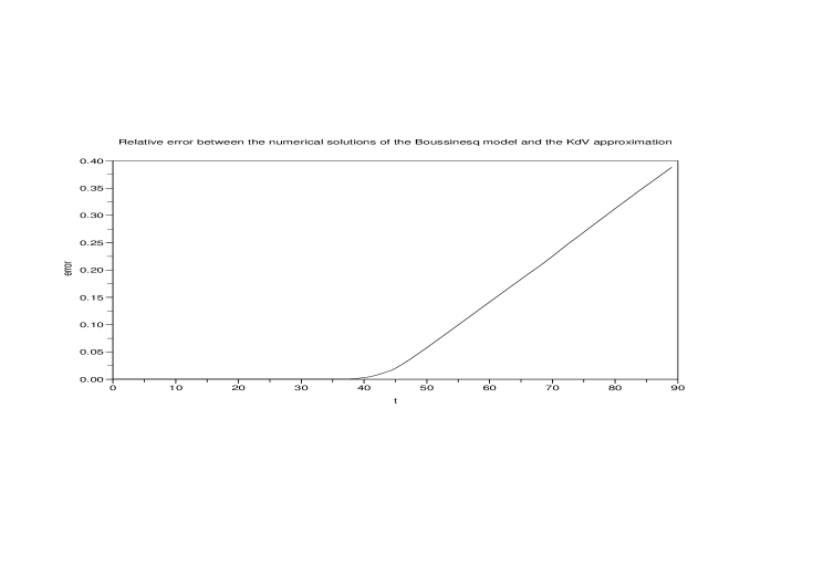
Figure 3.2.2: Relative $\displaystyle L^{\infty}$ error between the free surfaces for $\displaystyle\varepsilon=0.05$

Figure 3.2.3: Influence of the step for $\displaystyle\varepsilon=0.2$

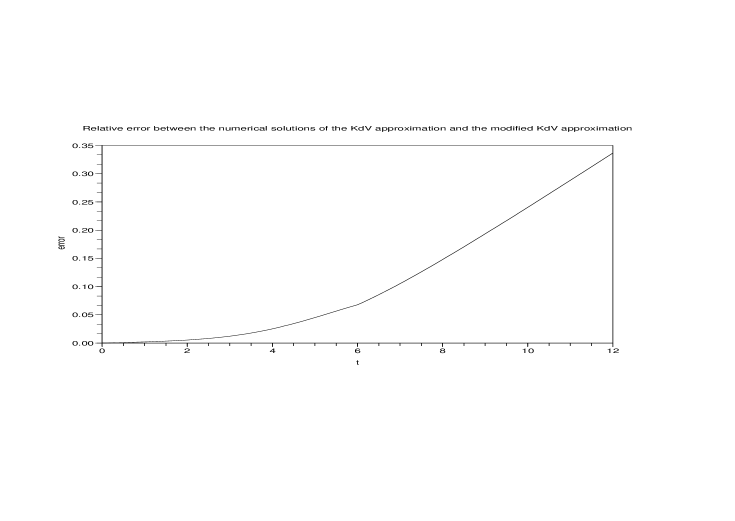
Figure 3.2.4: Relative $\displaystyle L^{\infty}$ error between the free surfaces for $\displaystyle\varepsilon=0.2$

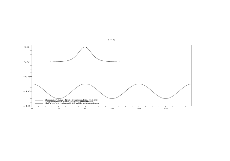
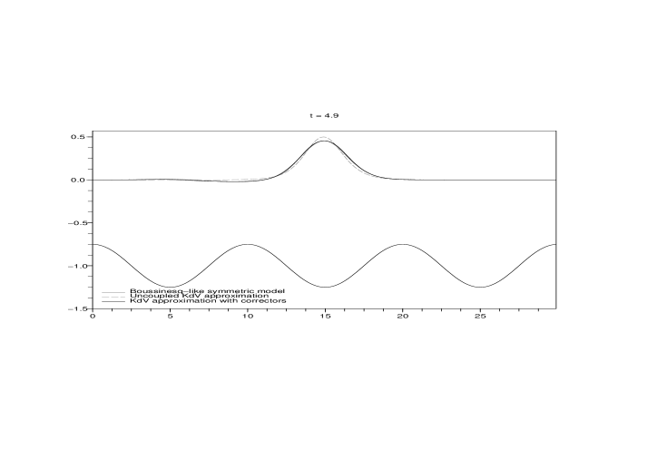
Figure 3.2.5: Influence of a slow sinusoidal bottom for $\displaystyle\varepsilon=0.1$

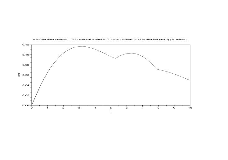
Figure 3.2.6: Relative $\displaystyle L^{\infty}$ error between the free surfaces for $\displaystyle\varepsilon=0.1$

3.2.2 Comments

For the sake of readability, we call the computed waves as follows : $\displaystyle\mathcal{B}$ denotes the wave coming from the Boussinesq model $\displaystyle(\Sigma)$, $\displaystyle\mathcal{K}_{topo}$ denotes the wave produced by the topographically modified KdV approximation $\displaystyle(\mathcal{M}_{b})$, and finally $\displaystyle\mathcal{K}$ denotes the solitary wave resulting from the usual KdV approximation $\displaystyle(\mathcal{M})$.

In the case of the step, we observe in figures 3.2.1 and 3.2.3 that for all tested values of $\displaystyle\varepsilon$, both the Boussinesq model and alternative version of the KdV approximation succeed in reproducing the phenomenon of reflexion on the bathymetry : a smaller solitary wave appears on the third snapshots when the main wave goes over the step. This reflected wave propagates to the left at the same speed as the main wave. The classical uncoupled KdV model cannot - of course - reproduce this phenomenon seing that it does not depend at all on the bottom topography. Moreover, the Boussinesq and topographically modified KdV models successfully describe the following expected physical phenomenons : the shoaling which corresponds to the growth in amplitude of the wave after the step ; the deceleration of the wave after the step : the waves $\displaystyle\mathcal{B}$ and $\displaystyle\mathcal{K}_{topo}$ are behind the wave $\displaystyle\mathcal{K}$ which propagates at a constant speed on the last snapshots of figures 3.2.1 and 3.2.3 ; and finally the loss of symmetry and the narrowing of the wave, which can be remarked by comparing - f.e. on the last snapshot of figure 3.2.3 - the distances between several points of the resulting waves at different heights : the solitary wave $\displaystyle\mathcal{K}$ propagates without any deformation and remains symmetric, whereas the symmetry and width of $\displaystyle\mathcal{B}$ and $\displaystyle\mathcal{K}_{topo}$ are modified by the step. All these phenomenons are the premisses of the process of wave breaking, and they are all successfully reproduced by the Boussinesq and new KdV models.

A very interesting remark on our KdV model is that the role of each correcting term in the approximation can be intuitively identified, and these intuitions have been confirmed with several simulations - that are not presented here - in the case of the step. Indeed, it appears clearly on figures 3.2.1 and 3.2.3 that :

• the correcting term $\displaystyle\frac{\varepsilon}{8}\int_{0}^{t}\partial_{x}b(x-t+s)U_{0}(x-t+2s)ds$ is responsible for the birth and propagation of the reflected wave, and for the very beginning of the shoaling effect,

• the correcting term $\displaystyle\frac{\varepsilon}{8}U_{0}(x-t)(b(x)-b(x-t))$ clearly reproduces the pursuit of the shoaling after the step,

• the correcting term $\displaystyle\frac{\varepsilon}{4}\partial_{x}U_{0}(x-t)\int_{0}^{t}b(x-t+s)ds$ is reponsible for the deceleration and loss of width and symmetry of the main wave after the step.

In the case of a slowly varying sinusoidal bottom - corresponding to figure 3.2.5 - the effect of the bottom is also clearly visible on $\displaystyle\mathcal{B}$ and $\displaystyle\mathcal{K}_{topo}$. To understand the speed variations of these waves, we have to keep in mind that the comparison is made with the wave $\displaystyle\mathcal{K}$ which evolves as if the bottom was flat and located at the height $\displaystyle y=-1$. Consequently, when $\displaystyle\mathcal{B}$ and $\displaystyle\mathcal{K}_{topo}$ propagate above the downward part of the sinusoidal gap - see second snapshot of 3.2.5 - they cross two different areas : a first area - for a time $\displaystyle t\leq T/4$ - where the depth is lower than for a flat bottom located at $\displaystyle y=-1$, and a second area - for $\displaystyle t\leq T/2$ - where this is the contrary. This explains why the waves $\displaystyle\mathcal{B}$ and $\displaystyle\mathcal{K}_{topo}$ are located for $\displaystyle t=T/2$ at the same position as $\displaystyle\mathcal{K}$ : the waves $\displaystyle\mathcal{B}$ and $\displaystyle\mathcal{K}_{topo}$ have speeded up over the first area in comparison with $\displaystyle(\mathcal{K})$, and then have decelerated over the second area. However, we can see - still on the second snapshot of 3.2.5 - that these waves are larger than $\displaystyle(\mathcal{K})$ at $\displaystyle t=T/2$ : this is due to the loss of amplitude of the waves $\displaystyle\mathcal{B}$ and $\displaystyle\mathcal{K}_{topo}$ during this downward part which makes the waves be naturally wider. About this loss of amplitude, it is explained by the fact that the amplitude of the bottom decreases over the downward part of the sinusoid, which produces the inverse effect of the shoaling from the previous case of the step. In addition, we can see a reflected wave for $\displaystyle\mathcal{B}$ and $\displaystyle\mathcal{K}_{topo}$ - a depression this time - which goes to the left at the same speed as the main wave, which corresponds to the same phenomenon of bathymetric reflexion as in the case of the step : the amplitude of the bottom decreases and thus produces a depression wave that propagates in the opposite direction. We can see that this depression wave is here larger than for a step because of the slow variations of the bottom. As far as the upward part - see last snapshot of 3.2.5 - of the sinusoid is concerned, all the previously described effects happen in an inverted way, and we finally recover three identical main waves for the three models. At this final point, the only remaining visible effects of the crossed topography are the reflected waves.

As specified earlier, we decided to simulate the models on the very large time $\displaystyle T=1/\varepsilon^{3/2}$ in the case of the step on figures 3.2.1 and 3.2.3. All these models have been proved to be valid on the time scale $\displaystyle O(1/\varepsilon)$ and it is interesting to check numerically their validity - or not - on larger time scales. For a time $\displaystyle T=1/\varepsilon^{3/2}$ , we can observe on the last two snapshots of figures 3.2.1 and 3.2.3 that the wave $\displaystyle\mathcal{K}_{topo}$ goes on growing more and more in amplitude, and that a depression wave deepens in front of the main wave. These effects are obviously not physical and can be explained by the fact that the size of the correcting term $\displaystyle\frac{\varepsilon}{4}\partial_{x}U_{0}(x-t)\int_{0}^{t}b(x-t+s)ds$ evolves in time like $\displaystyle\varepsilon/t$ as we saw in the previous section : on a time $\displaystyle T=1/\varepsilon^{3/2}$, this size become of order $\displaystyle O(1/\sqrt{\varepsilon})$, which explains why this model diverges from the other models on this time scale. This is the main restriction of this model, in comparison with the Boussinesq one which seems to remain stable on very large time scales. An interesting perspective would be to look for higher order terms - like Wright in [54] - in the approximation to deal with this problem.

To sum up, the results on these two examples of bottom show that both Boussinesq and topographically modified KdV models are able to reproduce the expected physical phenomenons : reflection, shoaling, loss of speed and symmetry. This is of course not the case for the usual KdV approximation which is independent from the bottom topography. Even if we can isolate the role of each correcting terms with our modified KdV aproximation, this one diverges when time goes over the theoretical limit time of validity $\displaystyle T=1/\varepsilon$. The Boussinesq does not have this drawback and remains stable on time scales of order $\displaystyle O(1/\varepsilon^{3/2})$.

Acknowledgments. This work was supported by the ACI Jeunes chercheurs du ministère de la Recherche “Dispersion et nonlinéarités”.

References

• [1] S. Alinhac, P. Gérard, Opérateurs pseudo-différentiels et théorème de Nash-Moser, Savoirs Actuels. InterEditions, Paris; Editions du Centre National de la Recherche Scientifique (CNRS), Meudon, 190 pp, 1991.
• [2] B. Alvarez-Samaniego, D. Lannes, Large time existence for 3D water-waves and asymptotics, Technical report (http://fr.arxiv.org/abs/math/0702015v1), Université Bordeaux I, IMB, 2007.
• [3] B. Alvarez-Samaniego, D. Lannes, A Nash-Moser theorem for singular evolution equations. Application to the Serre and Green-Naghdi equations, Preprint, to appear in Indiana University Mathematical Journal (http://arxiv.org/abs/math.AP/0701681v1), 2007.
• [4] D.M. Ambrose, N. Masmoudi, The zero surface tension limit of two-dimensional water waves, Comm. Pure Appl. Math., Vol. LVIII (2005), 1287-1315.
• [5] T.B. Benjamin, J.L. Bona, J.J. Mahony, Model equations for long waves in nonlinear dispersive systems, Philos. Trans. Roy. Soc. London Ser. A 272 (1972), 47-78.
• [6] C. Besse, Schéma de relaxation pour l’équation de Schrödinger non linéaire et les systèmes de Davey et Stewartson, C. R. Acad. Sci. Paris Sér. I, Vol. 326, No. 12, (1998) pp 1427-1432.
• [7] C. Besse, A relaxation scheme for Nonlinear Schrödinger Equation, Siam J. Numer. Anal., Vol. 42, No. 3, (2004), pp 934-952.
• [8] C. Besse, C.H. Bruneau, Numerical study of elliptic-hyperbolic Davey-Stewartson system : dromions simulation and blow-up, Mathematical Models and Methods in Applied Sciences, Vol. 8, No. 8 (1998) pp 1363-1386.
• [9] J.L. Bona, M. Chen, A Boussinesq system for two-way propagation of nonlinear dispersive waves, Physica D 116 (2004), 191-224.
• [10] J.L. Bona, M. Chen, J.C. Saut, Boussinesq Equations and Other Systems for Small-Amplitude Long Waves in Nonlinear Dispersive Media. I: Derivation and Linear Theory, J. Nonlinear Sci. 12 (2002), 283-318.
• [11] J.L. Bona, M. Chen, J.C. Saut, Boussinesq Equations and Other Systems for Small-Amplitude Long Waves in Nonlinear Dispersive Media. II: Nonlinear Theory, Nonlinearity 17 (2004), 925-952.
• [12] J.L. Bona, T. Colin, D. Lannes, Long Waves Approximations for Water Waves, Arch. Rational Mech. Anal. 178 (2005), 373-410.
• [13] J.L. Bona, R. Smith, The initial-value problem for the Korteweg-de Vries equation, Philos. Trans. Roy. Soc. London Ser. A, 278 (1975), 555-601.
• [14] J.V. Boussinesq Théorie de l’intumescence liquide appelée onde solitaire ou de translation se propageant dans un canal rectangulaire, C.R. Acad. Sci. Paris Sér. A-B 72 (1871), 755-759.
• [15] J.V. Boussinesq Théorie de des ondes et remous qui se propagent le long d’un canal rectangulaire horizontal, en communiquant au liquide contenu dans ce canal des vitesses sensiblement pareilles de la surface au fond, J. Math. Pures Appl. 17 (1872), no. 2, 55-108.
• [16] F. Chazel Influence of Bottom Topography on Long Water Waves, M2AN, 2007.
• [17] M. Chen, Equations for bi-directional waves over an uneven bottom, Mathematical and Computers in Simulation 62 (2003), 3-9.
• [18] W. Craig, An existence theory for water waves and the Boussinesq and Korteweg-de Vries scaling limits, Comm. Partial Differential Equations 10 (1985), no. 8, 787-1003.
• [19] W. Craig, P. Guyenne, D.P. Nicholls, C. Sulem, Hamiltonian long-wave expansions for water waves over a rough bottom, Proc. R. Soc. A 461 (2005) 839-873.
• [20] M.W. Dingemans, Water Wave Propagation over uneven bottoms. Part I: Linear Wave Propagation, Adanced Series on Ocean Engineering 13, World Scientific.
• [21] M.W. Dingemans, Water Wave Propagation over uneven bottoms. Part II: Nonlinear Wave Propagation, Adanced Series on Ocean Engineering 13, World Scientific.
• [22] D. Dutykh, F. Dias, Dissipative Boussinesq equations, Accepted to the special issue of C. R. Acad. Sci. Paris, dedicated to J.V. Boussinesq., 2007.
• [23] C. Fochesato, F. Dias, A fast method for nonlinear three-dimensional free-surface waves, Proceedings of the Royal Society of London A 462 (2001), 2715-2735.
• [24] A.E. Green, P.M. Naghdi, A derivation of equations for wave propagation in water of variable depth, J. Fluid Mech. 78 (1976), 237-246.
• [25] S. Grilli, P. Guyenne, F. Dias, A fully nonlinear model for three-dimensional overturning waves over arbitrary bottom, International Journal for Numerical Methods in Fluids 35 (2001), 829-867.
• [26] T. Iguchi, A long wave approximation for capillary-gravity waves and an effect of the bottom, Comm. Partial Differential Equations, 32 (2007), 37–85.
• [27] T. Iguchi, A mathematical justification of the forced Korteweg-de Vries equation for capillary-gravity waves, Kyushu J. Math., 60 (2006), 267-303.
• [28] R.S. Johnson, On the development of a solitary wave moving over an uneven bottom, Proc. Camb. Phil. Soc. 73 (1973), 183-203.
• [29] J.L. Joly, G. Métivier, J. Rauch, Generic rigorous asymptotic expansions for weakly nonlinear multidimensional oscillatory waves, Duke Math. J. 70 (1993), 373-404.
• [30] J.L. Joly, G. Métivier, J. Rauch, Diffractive nonlinear geometric optics with rectification, Indiana Univ. Math. J. 47 (1998), 1167-1241.
• [31] B.B. Kadomtsev, V.I. Petviashvili, On the stability of solitary waves in weakly dispersing media, Sov. Phys., Dokl. 15 (1970), 539-541.
• [32] T. Kakutani, Effect of an uneven bottom on gravity waves, J. Phys. Soc. Japan 30(1), 272-276, 1971.
• [33] T. Kato, On the Cauchy problem for the (generalized) Korteweg-de Vries equation, Studies in applied mathematics, 93-128. Advances in Mathematics, Supplementary Studies, 8. Academic, New York-London, 1983.
• [34] C.E. Kenig, G. Ponce, L. Vega, Well-posedness of the initial value problem for the Korteweg-de Vries equation., J. Amer. Math. Soc. 4 (1991), no. 2, 323-347.
• [35] J.T. Kirby, Gravity Waves in Water of Finite Depth, J. N. Hunt (ed). Advances in Fluid Mechanics, 10, 55-125, Computational Mechanics Publications, 1997.
• [36] D.G. Korteweg, G. de Vries On the change of form of long waves advancing in the rectangular canal and a new type of long stationary waves, Phil. Mag. 39 (1895), 422-443.
• [37] D. Lannes, Sur le caractère bien posé des équations d’Euler avec surface libre, Séminaire EDP de l’Ecole Polytechnique (2004), Exposé no. XIV.
• [38] D. Lannes, Well-posedness of the water-waves equations, J. Amer. Math. Soc. 18 (2005), 605-654.
• [39] D. Lannes, Secular growth estimates for hyperbolic systems, Journal of Differential Equations 190 (2003), no. 2, 466-503.
• [40] D. Lannes, J.C. Saut, Weakly transverse Boussinesq systems and the Kadomtsev-Petviashvili approximation, Nonlinearity 19 (2006) 2853-2875.
• [41] P.A. Madsen, R. Murray, O.R. Sorensen, A new form of the Boussinesq equations with improved linear dispersion characteristics (part 1), Coastal Eng. 15 (1991), 371-388.
• [42] G. Métivier, Small Viscosity and Boundary Layer Methods: Theory, Stability Analysis, and Applications, Modeling and Simulation in Science, Engineering and Technology, Birkhäuser, Boston-Basel-Berlin, 2004.
• [43] J.W. Miles, On the Korteweg-de Vries equation for a gradually varied channel, J. Fluid Mech. 91(1), 181-190, 1979.
• [44] V.I. Nalimov, The Cauchy-Poisson problem. (Russian) Dinamika Splošn. Sredy Vyp. 18 Dinamika Zidkost. so Svobod. Granicami, (1974), 104-210, 254.
• [45] A.C. Newell, Solitons in Mathematics and Physics, SIAM, Philadelphia, 244 pp., 1985.
• [46] D.P. Nicholls, F. Reitich A new approach to analyticity of Dirichlet-Neumann operators, Proc. Royal Soc. Edinburgh Sect. A, 131 (2001), 1411-1433.
• [47] O. Nwogu Alternative form of Boussinesq equations for nearshore wave propagation, J.Waterw. Port Coastal Eng. ASCE 119 (1993) No. 6, 618-638.
• [48] L.A. Ostrovskii, E.N. Pelinovskii, Refraction of nonlinear ocean waves in a beach zone, Izv., Atmos. and Oceanic Physics 6(9), 552-555, 1970.
• [49] D.H. Peregrine, Long waves on a beach, J. Fluid Mech., 27 (2005) No. 4, 815-827.
• [50] G. Schneider, C.E. Wayne, The long-wave limit for the water-wave problem. I. The case of zero surface tension., Comm. Pure Appl. Math., 162 (2002), no. 3, 247-285.
• [51] C.E. Wayne, J.D. Wright, Higher order corrections to the KdV approximations for a Boussinesq equation, SIAM Journal of Applied Dynamical Systems v. 1 (2002), 272-302.
• [52] G. Wei, J.T. Kirby A time-dependent numerical code for extended Boussinesq equations, Journal of Waterway, Port, Coastal and Ocean Engineering, 120 (1995), 251-261.
• [53] G. Wei, J.T. Kirby, S.T. Grilli, R. Subramanya, A fully nonlinear Boussinesq model for surface waves. I. Highly nonlinear, unsteady waves, Journal of Fluid Mechanics, 294 (1995), 71-92.
• [54] J.D. Wright, Corrections to the KdV approximation for water waves, SIAM Journal on Mathematical Analysis, v. 37, no. 4 (2005), 1161-1206.
• [55] S. Wu, Well-posedness in Sobolev spaces of the full water wave problem in $\displaystyle 2$-D, Invent. Math. 130 (1997), no. 1, 39-72.
• [56] S. Wu, Well-posedness in Sobolev spaces of the full water wave problem in $\displaystyle 3$-D, J. Amer. Math. Soc. 12 (1999), no. 2, 445-495.
• [57] H. Yosihara, Gravity waves on the free surface of an incompressible perfect fluid of finite depth. Publ. Res. Inst. Math. Sci. 18 (1982), no. 1, 49-96.