Application of afxy-code for parameterization of ionization yield function Y in the atmosphere for primary cosmic ray protons

Abstract

In this work is obtained new approximation for the yield function Y for cosmic ray induced ionization in the Earth atmosphere on the basis of simulated data. The parameterization is obtained using inverse nonlinear problem solution with afxy(analyze fx=y)-code. Short description of the methods is given. The found approximation is for primary proton nuclei, inclined up to 70 degrees zenith angle. This permits to estimate the direct ionization by primary cosmic rays explicitly. The parameterization is applicable to the entire atmosphere, from ground level to upper atmosphere. Several implications of the found parameterization are discussed.

Keywords:Cosmic Ray, Atmospheric Ionization, Inverse problem solution

Corresponding author:A.Mishev, INRNE-BAS, Tel: (+359) 29746310; e-mail: mishev@inrne.bas.bg

1 Introduction

Presently it is known that the Earth is hit by elementary particles and atomic nuclei of very large energies and in wide energy range, this is the cosmic ray radiation. The fluxes variate, from $10^{4}$ $m^{-2}$ $s^{-1}$ at energies $~{}10^{9}$ eV to $10^{-2}$ $km^{-2}$ $yr^{-1}$ at energies $~{}10^{20}$ eV. The cosmic ray intensity is approximatively expressed with (1), where E is the total particle energy per nucleon in GeV and $\alpha=-2.7$ is the spectral index. The majority of these particles are protons. The primary cosmic rays penetrate upper atmosphere, secondary cosmic rays are produced by the interactions of primary rays in the atmosphere.

$$I_{n}(E)\varpropto 1.8(\frac{E}{GeV})^{\alpha}nucleons.cm^{-2}.s^{-1}.sr^{-1}$$ (1)

The abundances are approximately independent of energy, at least over the dominant energy range of 10 MeV/nucleon through several GeV/nucleon. By mass about 79 percent of nucleons in cosmic rays are free protons, and about 80 percent of the remaining nucleons are bound in helium.

There are three different types of cosmic rays: galactic cosmic rays, solar cosmic rays and anomalous cosmic rays. Most galactic cosmic rays are accelerated in the shock waves of supernova remnants. Because of their deflection by magnetic fields, galactic cosmic rays follow convoluted paths and arrive at the top of the Earth’s atmosphere in practice uniformly from all directions. Galactic cosmic rays are the most typical cosmic rays, and their flux in the solar system is modulated by the solar activity: enhanced solar wind shields the system from these particles [1].

We know that the galactic cosmic rays create the ionization in the stratosphere and troposphere and also in the independent ionosphere layer at altitudes 50-80 km in the D region [2]. This ionization is a result from the impact of the secondary cosmic ray electromagnetic, muon and hadronic components on the planetary atmosphere. The cosmic ray induced ionization is an important factor of space influences on atmospheric properties.

In general the variations of cosmic ray induced ionization are caused by solar activity variations, which modulate the cosmic ray flux in interplanetary space, and changes of the geomagnetic field, which affects the cosmic ray penetration in the atmosphere and their access to Earth. The changing solar activity is responsible for the variation of solar wind, respectively cosmic rays. The solar wind reduces the flux of cosmic ray reaching the Earth, since a larger amount of energy is lost as they propagate up the solar wind. Since cosmic rays dominate the ionization, an increased solar activity will translate into a reduced ionization.

On the basis of satellite data analysis was shown that cloud cover varies with the variable cosmic ray flux reaching the Earth [3, 4]. Over the relevant time scale, the largest variations arise from the 11-yr solar cycle, and indeed, this cloud cover seemed to follow the cycle and a half of cosmic ray flux modulation. Specifically was shown that the correlation is primarily with low altitude cloud cover [5].

In this connection a detailed model of the cosmic ray induced ionization will be a good basis for a quantitative study of different mechanisms affecting Earth’s atmosphere. To estimate the cosmic ray induced ionization it is possible to use a model based on an analytical approximation of the atmospheric cascade [6] or on a Monte Carlo simulation of the atmospheric cascade [7, 8]. A key issue, which allows to estimate the cosmic ray induced ionization for given location, altitude and spectrum of cosmic rays is the use of ionization yield function Y (2) which is defined according [9]

$$Y(x,E)=\triangle E(x,E)\frac{1}{\triangle x}\frac{1}{E_{ion}}\Omega$$ (2)

where $\triangle E$ is the deposited energy in layer $\triangle x$ in the atmosphere and $\Omega$ is a geometry factor, integration over the solid angle with zenith of 70 degrees. Afterwards the ion pair production q by cosmic rays following steep spectrum is easy calculated according the expression:

$$q(h,\lambda_{m})=\int D(E,\lambda_{m})Y(h,E)\rho(h)dE$$ (3)

where $D(E,\lambda_{m})$ is the differential primary cosmic ray spectrum at given geomagnetic latitude, Y is the yield function according (2), $\rho(h)$ is the atmospheric density in [$g.cm^{-3}$].

The ionization yield function Y depends only of assumed physical models for cascade processes in the atmosphere, the atmospheric model and the type of the primary particle. Therefore having a convenient parameterization for ionization yield function Y and parameterized differential energy spectrum of galactic cosmic rays at the Earth’s orbit it is possible to estimate cosmic ray induced ionization in different locations and conditions. In this work we use the previously obtained ionization yield function Y [10, 11] for primary protons.

The major contribution of cosmic ray induced ionization in the atmosphere is due to particles having energy till 1 TeV, taking into account the steep spectrum of primary cosmic rays (1). This is the reason to deal in this paper with primary protons with maximal energy of 1 TeV.

2 How to investigate a given nonlinear system

Many problems in physics, applied mathematics even and pure mathematics lead to solution of nonlinear system of equation.

To analyze nonlinear equation, we write it in the form

$$fx=\overline{y},\quad f:D_{f}\subset\mathbb{R}^{n}\to\mathbb{R}^{m},\;x\in\mathbb{R}^{n},\;\overline{y}\in\mathbb{R}^{m}.$$ (4)

To analyze iteratively nonlinear systems involves two related classes of problems [12]- heuristic investigation of nonlinear systems issuing from not-refined mathematical models and automatic solution of streams of one-type nonlinear systems of equations.

2.1 Main iteration procedure in afxy-code[12]

A powerfull tool for an heuristic analysis of systems of nonlinear equations (4) is afxy-code (analyze fx=y).In the case $n\leq m$ as well in non-trivial case $n>m$ we employ regularized Gauss-Newton type iterator

$$\overline{x}\in D_{f},\;x^{0}\in D_{f},\;\epsilon^{0}>0,\quad({f^{\prime}}^{T}(x^{k})f^{\prime}(x^{k})+(\epsilon^{k}+\alpha^{k})I)(x^{k+1}-x^{k})=$$ (5)

$$-{f^{\prime}}^{T}(x^{k})(fx-\overline{y})-\alpha^{k}\overline{x}),\;k=0,1,\ldots\;.$$

The regularizators $\varepsilon^{k}$ (of the process) and $\alpha^{k}$ (of the problem) will be defined below.

In the right hand of (5) original problem (4) is transformed by Gauss manner $Fx:=f^{{}^{\prime}T}(x)(fx-\overline{y})$ and additively regularized by von Neumann-Tichonov manner. The space $\mathbb{R}^{n}$ we consider as a two different normed elementwise equal spaces $\mathbb{R}^{n}_{\infty}$ and $\mathbb{R}^{n}_{2}$.

The space $\mathbb{R}^{n}_{\infty}$ is normed by $L_{\infty}$ norm $\|a\|_{\infty}=\max\limits_{i}|a_{i}|$, $(a=[a_{1},a_{2},...,a_{n}]^{T}\in\mathbb{R}^{n})$ and $\mathbb{R}^{n}_{2}$ space is normed respectively by $L_{2}$ norm $\|a\|_{2}=(\sum_{i=1}^{n}a_{i}^{2})^{\frac{1}{2}}$.

The corresponding matrix spaces $[\mathbb{R}^{n}_{\infty},\mathbb{R}^{n}_{\infty}]$ and $[\mathbb{R}^{n}_{2},\mathbb{R}^{n}_{2}]$ are normed respectively by $\|A\|_{\infty}=\max\limits_{i}\sum_{j=1}^{n}|a_{ij}|$, $A=\{a_{i,j}\}\in[\mathbb{R}^{n}_{\infty},\mathbb{R}^{n}_{\infty}]$ and by $\|A\|_{2}=\lambda_{m}$, where $\lambda_{m}$ is the maximal spectral number of the matrix A [13]. Note, the norm $\|A\|_{\infty}$ is well defined. It is simultaneously completed and consisted to the vector norm $\|a\|_{\infty}$.

The iterator (5) produces two different approximating sequences subjects to the used regularizators.

To solve an ill-conditioned [14] problem (4) we use the process (5) in the $\mathbb{R}^{n}_{\infty}$ space with autoregularizator of the process [15, 16]

$$\epsilon^{k}=\frac{1}{2}\left(\sqrt{(\tau^{k})^{2}+4N\rho^{k}}-\tau^{k}\right),$$ (6)

where $\tau^{k}=||{f^{\prime}}^{T}(x^{k})f^{\prime}(x^{k})||_{\infty},\quad\rho^{k}=||{f^{\prime}}^{T}(x^{k})(fx^{k}-\overline{y})||_{\infty}$ and $N=const>0$. The behavior of the autoregularizator is accordant semilocal convergence [16] of the process (5). As a rule the convergence domain expands with increasing the initial value of the regularizator $\varepsilon^{0}$.

To solve a singular problem [14](4), we use the process (5) in the space $\mathbb{R}^{n}_{2}$ with autoregularizator (6) with

$$\tau^{k}=\lambda^{k}_{m}$$ (7)

is the smallest non-negative eigenvalue of the matrix ${f^{\prime}}^{T}(x^{k})f^{\prime}(x^{k})$ and

$$\rho^{k}=||{f^{\prime}}^{T}(x^{k})(fx^{k}-\overline{y})-\alpha{{}^{k}}\overline{x})||_{2},\;\alpha{{}^{k}}=\gamma exp(-\sigma(k-1)),\;\gamma,\sigma={\it const}\geq 0.$$ (8)

Presently in the case of singular problem we have not good semilocal theory for the convergence of the process (5)-(8). In the case of when convergence persists to a point $x^{*}$, the value $\|x^{*}-\overline{x}\|_{2}$ is minimal. Usually one takes $\overline{x}=0$. However the proposed iterator is fully applicable and was used for analysis of large diversity of problems.

The described main iteration procedure starting from Levenberg-Marquardt years till present days was applied extremely successful.

2.2 From local root extractors to global iterative processes

In order to find all solutions of Eq. (4) in the domain $D_{f}$ the vector $Fx^{k}$ is repeatedly multiplied by the local root extractor

$$e^{j}(x,\bar{x}^{(j)})=\frac{1}{1-\exp\left(-||x-\bar{x}^{(j)}||_{2}^{2}\right)},$$

in which $\bar{x}^{(j)}$ is the $j$-th solution of Eq. (4). In the repeated solutions of the transformed problem

$$F^{J}x:=\left(\prod_{j=1}^{J}e^{j}(x,\bar{x}^{(j)})\right)Fx=0,\quad J\geq 1,$$ (9)

the process (5) is executed with a new $Fx:=F^{J}x$. For every solution the process (5) is started many times with different $x^{0}$ and $\epsilon^{0}$. Each time when $J$ increases the derivatives $f^{\prime}(x^{k})$ are computed analytically and the matrices ${f^{\prime}}^{T}(x^{k})f^{\prime}(x^{k})$ are adaptively scaled.

To analyze globally nonlinear problem (4) means to find all solutions with estimation of themselves isolation in the domain $D_{f}$. For this purpose was build the mentioned above local root extractor.

3 The parameterization of ionization yield function Y

The ionization yield function Y gives the number of ion pairs, produced in 1 g of the ambient air at a given atmospheric depth by one particle of the primary cosmic ray radiation with given kinetic energy per nucleon.

The approximation is obtained following procedures similar to described in [17, 18]. In this case we take the logarithm of the problem, which permits to approximate large diversity of distributions with similar shapes, having different amplitudes with one model function with different parameters [19, 20, 21].

3.1 Approximation of ionization yield function Y

Usually the proposed approximation are carried out with large diversity and classes of functions, some very complicated. It exist powerful class of approximations - fractional-rational functions applied in our case. As a result we obtain description of the simulated data and fast convergence of the iteration process. For example we utilize simple fractional-rational function

$$Y(h)=\frac{ah^{2}+bh+c}{dh^{2}+eh+f}$$ (10)

where h is the atmospheric depth and a,b,c,d,e and f are parameters. The fits for ionization yield function Y are presented in Fig.1-8 for protons with energies 500 MeV, 1 GeV, 5 GeV, 10 GeV, 50 GeV, 100 GeV, 500 GeV and 1 TeV. In the figures with solid black squares are shown the obtained approximations and with open circles the simulated data. During the solution of the inverse problem we take logarithm of problem and scaling of the argument. This permits to obtain parameterization with small uncertainties and fast convergence of the process. In this case we solve ill-conditioned problem with large number of condition $10^{17}$. The solution is obtained after only 100 iterations steps. In this case the normalized $\chi^{2}$ varies between 0.13 for 500 MeV protons and 0.001 for 1 TeV protons.

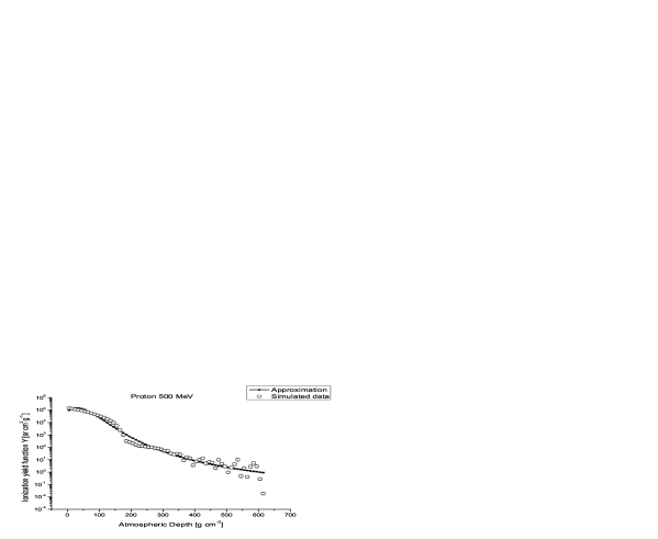
Figure 1: Approximation of ionization yield function Y for 500 MeV primary protons

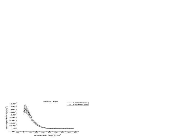
Figure 2: Approximation of ionization yield function Y for 1 GeV primary protons

Figure 3: Approximation of ionization yield function Y for 5 GeV primary protons

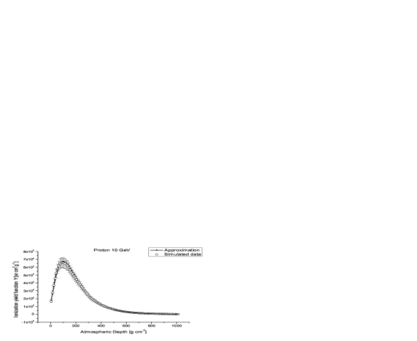
Figure 4: Approximation of ionization yield function Y for 10 GeV primary protons

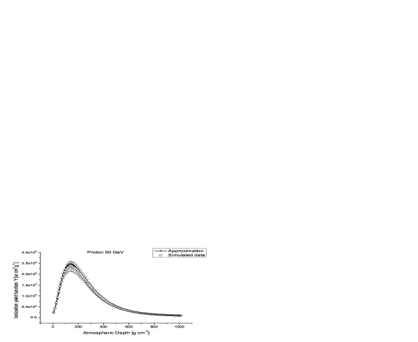
Figure 5: Approximation of ionization yield function Y for 50 GeV primary protons

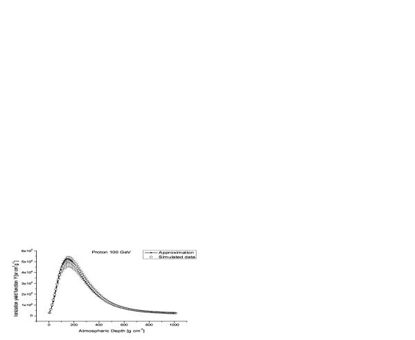
Figure 6: Approximation of ionization yield function Y for 100 GeV primary protons

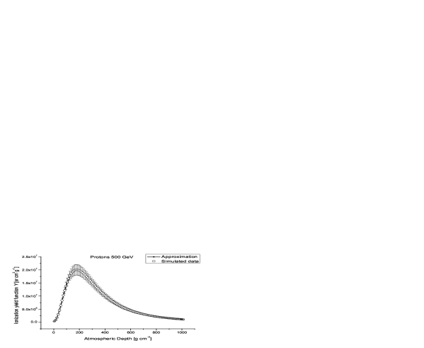
Figure 7: Approximation of ionization yield function Y for 500 GeV primary protons

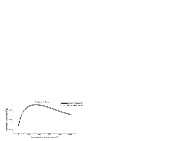
Figure 8: Approximation of ionization yield function Y for 1 TeV primary protons

3.2 Main results and parameters

The quality of the parameterization is the same in all cases.

The general aim is in one hand the precise description of the position of the Pfotzer maximum and on the other hand good description in the low atmosphere.

In the case of ionization yield function for 500 MeV protons Fig.1 the end points of the distribution are equally weighted. Our approximation is chosen to take the mean values at distribution tail.

In the remain cases the main difficulties are connected with precise description of the Pfotzer maximum. As example for the ionization yield function for 1 GeV and 5 GeV protons on observes very good coincidence between approximation and simulated data (see Fig. 2 and Fig.3). The approximated ionization yield function for 10 GeV protons coincides with simulated data (Fig.4).

In the case for 50 and 100 GeV, the parameterization gives slight increase of ion pairs in Pfotzer maximum (Fig. 5 and Fig.6).

Finally in the case of ionization yield function for 500 GeV and 1 TeV protons the approximation coincides once more with simulated data (Fig. 7 and Fig.8).

In all cases the approximation in practice coincides with simulated data in all other regions of the atmosphere,especially in the lower atmosphere. The parameters of the approximation are presented in Table.1.

Table 1: The parameters of the approximation

Energy	a	b	c	d	e	f
500 MeV	-6.09548	3.14499	0.31817	2.76023	0.37625	0.06494
1 GeV	-2.51931	3.81687	0.78784	1.0136	0.64061	0.15493
5 GeV	-4.55444	6.69186	0.47114	0.2117	1.0687	0.09188
10 GeV	-0.89284	4.01468	0.19579	0.30881	0.5975	0.03812
50 GeV	1.82327	2.46817	0.15813	0.55512	0.31109	0.02995
100 GeV	2.28484	1.99474	0.13683	0.56878	0.22815	0.0255
500 GeV	0.99557	2.65916	0.10061	0.29285	0.30755	0.01891
1 TeV	0.03717	2.72562	0.24925	0.13949	0.27453	0.04701

The approximation parameters are easy to fit with exponential or power low functions. This permits using the expression for ionization (3) to estimate the cosmic ray induced ionization at given location and altitude.

In addition, it is important that the approximation (10) is analytically integrable , which gives the possibility to estimate the total atmospheric ionization explicitly.

4 Discussion

The obtained parameterization of ionization yield function Y permits easily to compute the ionization rates from cosmic rays in the Earth atmosphere for given location and conditions, instead of using counting rates from different devices as a proxy. Moreover the parameterization allows to estimate variations of the cosmic ray induced ionization caused by the variable solar activity and as result to evaluate several atmospheric effects of cosmic rays, on different timescales and under different heliospheric conditions.

The cosmic rays may affect climate, and are probably important climate driver. Recently, it was shown in [22] that the variations in the amount of cloud cover follow the expectations from a cosmic-ray cloud cover link, specifically for low altitudes [5]. It was shown that the relative change in the low altitude cloud cover is proportional to the relative change in the solar-cycle induced atmospheric ionization at the given geomagnetic latitudes. Namely, at higher latitudes the ionization variations are about twice as large as those of low latitudes.

Above 100 percent saturation, the phase of water is liquid and it will not be able to condense unless it has a surface to. Therefore for formation of cloud droplets the air must have cloud condensation nuclei. Changing the density of these particles, the properties of the clouds can be varied. Having more cloud condensation nuclei, the cloud droplets are more numerous but smaller, this tends to make whiter and longer living clouds. The suggested hypothesis, is that in regions devoid of dust, the formation of cloud condensation nuclei takes place from the growth of small aerosol clusters, and that the formation of the latter is governed by the availability of charge, such that charged aerosol clusters are more stable and can grow while neutral clusters can more easily break apart.

If this process is dominant, charge and therefore cosmic ray ionization would play an important role in the formation of cloud condensation nuclei. With this in mind assuming our parameterization (10) for ionization yield function Y and relation (3), as well the parameterization for differential cosmic ray spectrum [23] we estimate the ionization rates for several cut-off rigidities (Fig.9).

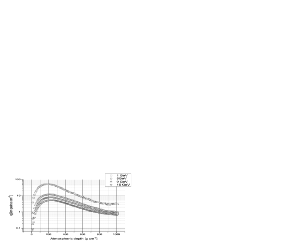
Figure 9: Ion pairs for Proton induced showers for 1, 5, 9 and 15 GV rigidities

The presented results demonstrate realistic cosmic ray induced ionization profile using average primary cosmic ray spectrum during moderate solar activity. As it is seen these results are applicable for different geomagnetic latitudes, respectively different locations. The obtained results are in good agreement with the profiles described in [9, 11].

It exists the hypothesis that the intrinsic variation in the cosmic ray flux are clearly evident in the geological paleoclimate data. Within the determinations of the period and phase of the spiral-arm climate connection, the astronomical determinations of the relative velocity agree with the geological sedimentation record for when Earth was in a hothouse or icehouse conditions [24]. Moreover, it was found that the cosmic ray flux can be independently reconstructed using the so called ”exposure ages” of Iron meteorites [25].

Thus it is very important, in one hand to investigate the hypothetic influence of cosmic rays on the Earth’s climate trough the mechanism cosmic rays induced ionization-condensation nuclei-cloud condensation nuclei-cloud cover, and on the other hand to study the impact of intrinsic variation in the cosmic ray flux during the motion of our planet in the Galaxy in attempt to estimate and clarify their contribution.

5 Conclusions

In this work is presented new convenient parameterization of the yield ionization function Y of primary cosmic rays into the Earth atmosphere. The parameterization was obtained on the basis of inverse problem solution using afxy-code.

The importance of cosmic ray induced ionization is widely discussed, precisely the mechanism related to clod cover formation.

Our results are important for precise estimation of the ionization profiles in the atmosphere, when one deal with proton nuclei from primary cosmic ray.

Acknowledgments
The authors thank the Bogolubov Laboratory of Theoretical Physics JINR, Dubna for hospitality and support, especially Prof. V. B. Priezzhev. We acknowledge our colleagues from Solar-Terrestrial Influences Laboratory - Bulgarian Academy of Sciences. We warmly acknowledge Prof. V. Yanke and Dr. E. Eroshenko as well as Prof. L. Miroshnichenko from IZMIRAN Russia for the fruitful discussions. Finally we thank Dr. I. Usoskin from Oulu university for several suggestions.

References

- [1] S. Forbush, Worldwide cosmic ray variations, 1937-1952. Journal of Geophysical Research 59, 525-542 (1954)
- [2] P. Velinov et al. Cosmic Ray Influence on the Ionosphere and on the Radio-Wave Propagation. BAS Publ. House, Sofia, 1974
- [3] H. Svensmark and E. Friis-Christensen, Variation of cosmic ray flux and global cloud coverage a missing link in solar-climate relationships. Journal of Atmospheric and Solar-Terrestrial Physics, 59(11), 1225-1232 (1997)
- [4] B. Tinsley, Correlations of atmospheric dynamics with solar wind-induced changes of air-earth current density into cloud tops. Journal of Geophysical Research 101(29), 701-714 (1996)
- [5] N. Marsh and H. Svensmark, Low cloud properties influenced by cosmic rays. Physical Review Letters 85, 5004 (2000)
- [6] K. O’Brien, Proceedings of the 7th International Symposium on the Natural Radiation Environment, 29- 44 (2005)
- [7] I. Usoskin., O. Gladysheva and G. Kovaltsov, Cosmic ray-induced ionization in the atmosphere: spatial and temporal changes. Journal of Atmospheric and Solar Terrestrial Physics 66(18), 1791- 1796 (2004)
- [8] L . Desorgher et al., Atmocosmics: A GEANT 4 code for computing the interaction of cosmic rays with the Earth’s atmosphere. Internatinal Journal of Modern Physics A, 20, 6802- 6804 (2005)
- [9] I. Usoskin and G. Kovaltsov, Cosmic ray induced ionization in the atmosphere: Full modeling and practical applications. Journal of Geophysical Research. 111, D21206 (2006)
- [10] A. Mishev and P. I.Y. Velinov, Atmosphere Ionization Due to Cosmic Ray Protons Estimated with Corsika Code Simulations. Comptes rendus de l’Academie bulgare des Sciences, 60(3), 225-230 (2007)
- [11] P.I.Y. Velinov and A. Mishev, Cosmic Ray Induced Ionization in the Atmosphere Estimated with CORSIKA Code Simulations. Comptes rendus de l’Academie bulgare des Sciences, 60(5), 493-500 (2007)
- [12] L. Alexandrov, Unified code for heuristic investigation and automatic solution of nonlinear systems of equations. http://www.math.nsc.ru/conference/ipmp07/abstracts/Section3/AlexandrovL.doc, (2007)
- [13] L. Collatz, Funktionanalysis und Numerische Mathematik. Springer Berlin (1964)
- [14] A. Tikhonov and V. Arsenin, Methods for the Solution of Noncorrect Problems, Nauka, Moskow, 1979.
- [15] L. Alexandrov, Newton-Kantorovich type autoregularized iteration processes. Communications of JINR Dubna P5 5515, Dubna, 1970
- [16] L. Alexandrov, Regularized numerical Newton-Kantorovich type processes.Journal of Computational Mathematics and Mathematical Physics 11(1), 36-43 (1971)
- [17] L. Alexandrov, M. Brankova, I. Kirov, S. Mavrodiev, A. Mishev, J. Stamenov and S.Ushev,A Possible estimation of atmospheric Cherenkov light parameters. Communications of JINR Dubna E2 -98-48, Dubna, 1998
- [18] L. Alexandrov M. Brankova, I. Kirov, S. Mavrodiev, A. Mishev, J. Stamenov and S.Ushev, Estimation of primary cosmic ray charateristics with the help of EAS Cherenkov light. Communications of JINR Dubna E2 -99-233, Dubna, 1999
- [19] A. Mishev, S. Mavrodiev and J. Stamenov, Primary Cosmic Ray Studies Based on Atmospheric Cherenkov Light Technique at High-Mountain Altitude. Frontiers in Cosmic Ray Research (Nova Science) ISBN: 1-59454-793-9, 35-82 (2007)
- [20] A. Mishev S. Mavrodiev and J. Stamenov, Ground based Gamma Ray Studies based on Atmospheric Cherenkov technique at high mountain altitude. International Journal of Modern Physics A, 20(29), 7016-7019 (2005)
- [21] S. Mavrodiev A. Mishev and J. Stamenov, A method for energy estimation and mass composition determination of primary Cosmic rays at Chacaltaya observation level based on atmospheric Cerenkov light technique. Nuclear Instruments and Methods A 530, 359-366 (2004)
- [22] I. Usoskin, N. Marsh, G.A. Kovaltsov, K. Mursula and O. Gladysheva, Latitudinal dependence of low cloud amount on cosmic ray induced ionization.Geophysical Research Letters 31, L16109 (2004).
- [23] M. Buchvarova and P.I.Y. Velinov, Modeling spectra of cosmic rays influencing on the ionospheres of the earth and outer planets during solar maximum and minimum. Advances in Space Research, 36(11), 2127-2133 (2005)
- [24] N. Shaviv, The spiral structure of the Milky Way, cosmic rays, and ice age epochs on Earth. New Astronomy 8, 39 (2003)
- [25] N. Shaviv, Cosmic Ray Diffusion from the Galactic Spiral Arms, Iron Meteorites, and a Possible Climatic Connection. Physical Review Letters 89, 051102 (2002).