Formation and transformation of the 3:1 mean-motion resonance in 55 Cancri System

Abstract

We report in this paper the numerical simulations of the capture into the 3:1 mean-motion resonance between the planet b and c in the 55 Cancri system. The results show that this resonance can be obtained by a differential planetary migration. The moderate initial eccentricities, relatively slower migration and suitable eccentricity damping rate increase significantly the probability of being trapped in this resonance. Otherwise, the system crosses the 3:1 commensurability avoiding resonance capture, to be eventually captured into a 2:1 resonance or some other higher-order resonances. After the resonance capture, the system could jump from one orbital configuration to another one if the migration continues, making a large region of the configuration space accessible for a resonance system. These investigations help us understand the diversity of resonance configurations and put some constrains on the early dynamical evolution of orbits in the extra-solar planetary systems.

1 Introduction

Up to date, more than 200 extra-solar planetary systems have been found. Those hosting more than one planet are multiple planet systems. In some of the multiple planet systems, planets are observed to be locked in mean-motion resonance (MMR), for example, the well-known 2:1 MMR in GJ876 system (e.g. [Marcy et al. (2001), Marcy et al. 2001]) and the 3:1 MMR in 55 Cancri system (e.g. [Zhou et al. (2004), Zhou et al. 2004]). In a 3:1 MMR, at least one of the three resonant angles ($\theta_{1}=\lambda_{1}-3\lambda_{2}+2\varpi_{1}$, $\theta_{2}=\lambda_{1}-3\lambda_{2}+2\varpi_{2}$, $\theta_{3}=\lambda_{1}-3\lambda_{2}+\varpi_{1}+\varpi_{2}$) librates, where $\lambda_{1,2}$ and $\varpi_{1,2}$ are the mean longitudes and periastron longitudes of the inner and outer planet respectively. The resonant systems are particularly attractive because not only of the complicated dynamics of the resonance but also of interesting information about its origin and early evolution buried in the configuration and dynamics.

The 55 Cancri system is the only example of 3:1 MMR found in the extra-solar planetary systems till now. Four planets have been reported in this system and two of them, 55 Cnc b and 55 Cnc c, seem to be locked in a 3:1 MMR. In our previous work, we have found that they are most likely in one of the three possible configurations ([Zhou et al. (2004), Zhou et al. 2004]). G.Marcy declared in his lecture in this Symposium that a fifth planet has been dug out from observing data of this system, enriching the whole story with more connotations. In the dynamical simulations of their 5-planet solution ([Fischer et al. (2007), Fischer et al. 2007]), they did not found the resonance between the two planets, although their orbital periods are very close to the 3:1 commensurability. However, the current orbit determinations may not be robust enough to determine the resonant angles, especially for orbits with low eccentricities as be given in this new determination, thus the resonant character of this pair of orbits may change as more observations are included ([Beaugé (2008), Beaugé 2008]). Furthermore, what we will discuss in this paper has some general significance so that we may still adopt the orbital elements and planetary masses from the previous literature ([McArthur et al. (2004), McArthur et al. 2004]), as listed in Table 1

Table 1: Orbital elements and masses. The mass of the central star is $1.03M_{\odot}$ ([McArthur et al. (2004), McArthur et al. 2004]). In this paper we adopt the planet masses by assuming $\sin i=1$.

Parameter	Cancri e	Cancri b	Cancri c	Cancri d
$M\sin i$ $(M_{J})$	0.045	0.784	0.217	3.92
$P$ (days)	2.81	14.67	43.93	4517.4
$a$ (AU)	0.038	0.115	0.240	5.257
$e$	0.174	0.0197	0.44	0.327

It is widely accepted that a planet may experience (generally inward) migration, and through differential migrations of planets, different commensurabilities among planets can be attained (e.g. [Nelson & Papaloizou (2002), Nelson & Papaloizou 2002]). For example, the 2:1 MMR in GJ876, whose configuration can be obtained through the inward migration of the outer planet ([Lee & Peale (2002), Lee & Peale 2002]).

On the other hand, the resonant capture probability depends on the order of the resonance, the migration rate and the initial planetary eccentricity ([Quillen (2006), Quillen 2006]). The formation process of the 3:1 MMR may be very different from the one of the 2:1 MMR. As the only example of 3:1 MMR in extra-solar planetary systems, the 55 Cancri system deserves a detailed investigation. In this paper, we will report our numerical simulations of the capture into resonance, and the evolution of the resonance thereafter, provided the migration continues.

2 Numerical simulations of resonance formation

There are more planets than the two (planet b and c) in our focus of attention in this planetary system. However, besides these two planets, the massive one (55 Cnc d) is too far and the close one (55 Cnc e) is too small. Moreover, even the newly reported planet (55 Cnc f) is neither very massive ($M_{f}\sin i=0.144M_{\rm Jup}$) nor very close to this planet pair ($a_{f}=0.781$ AU, $P_{f}=260$ days). Therefore as a simplified model, it is reasonable to discuss only the two planets under the influences of the central star and the disc.

2.1 Numerical Model

As usual, the influence of the disc on the planets is simply simulated by an artificial force, which is acting on the outer planet to drive it to migrate inward. The force is defined so that the semi-major axis of the planetary orbit will change following an exponential law:

$$a(t)=a_{0}+\Delta a\times e^{-t/\tau}.$$ (1)

where $a_{0}$ is the initial semi-major axis of the planet, and $\tau$ is the timescale of the migration. The two planets are assumed to be located initially on orbits with semi-major axes of 1.25 AU and 0.5 AU, with an initial semi-major axes ratio of 2.5 (periods ratio 3.95), which will evolve downward to the value corresponding to the 3:1 MMR (2.08). Obviously the value of $\tau$ determines the migration speed. The smaller the $\tau$, the faster the migration, and vice versa. Different $\tau$ values were adopted in different papers. The standard migration scenario (type II) gives an estimate of migration rate ([Ward (1997), Ward 1997]):

$$\left|\frac{\dot{a}}{a}\right|=9.4\times 10^{5}\left(\frac{\alpha}{4\times 10^{-3}}\right)\left(\frac{H/a}{0.05}\right)^{2}P^{-1}.$$ (2)

Taking the typical parameters $\alpha$ and $H/a$, the $\tau$ for a planet starting from 1.25 AU is $\sim 1.43\times 10^{4}$ yrs. Some other rules have been applied in different papers. According to these rules, the $\tau$ would be, for example, $1.56\times 10^{4}$ yrs ([Lee & Peale (2002), Lee & Peale 2002]), $1.38\times 10^{4}$ yrs ([Nelson & Papaloizou (2002), Nelson & Papaloizou 2001]), and $2.65\times 10^{4}$ yrs ([Kley (2003), Kley 2003]; [Kley, Peitz & Bryden (2004), Kley et al. 2004]). In our simulations, it is set to be $2\times 10^{4},1\times 10^{5},2\times 10^{5}$ and $5\times 10^{5}$ yrs. Some large values (meaning slow migration) are adopted here to guarantee the capture into the 3:1 MMR.

Although it is still not very clear now how a certain disk will damp or stimulate the eccentricity of an embedded planet, people hope the disk will circularize an orbit if it was too eccentric. In order to control the unlikely eccentricity increasing during the artificially induced migration, we have included an eccentricity-damping force in our simulations. A parameter $K$ was introduced to describe the damping rate, with which we control the eccentricity $e$ of a planet by:

$$\left|\dot{e}/e\right|=K\left|\dot{a}/a\right|.$$ (3)

In our simulations, the parameter $K$ has the values 0 (no damping), 1, 10 and 100. The damping is always put on planet 55 Cnc c with the migrating force modifying its semimajor axis simultaneously.

In the simulations, the two orbits are nearly coplanar (in the practice of numerical simulations we adopt an arbitrarily defined small inclination between these two orbits, say 0.1 degree), and the initial orbital eccentricities of planet 55 Cnc b ($e_{1}^{0}$) and 55 Cnc c ($e_{2}^{0}$) are set to be $0.001$ (a typical value for a nearly circular orbit) as well as $0.01,0.05,0.1,0.2$. For each mode (with certain $\tau,K,e_{1}^{0},e_{2}^{0}$), we numerically integrate 100 systems with randomly selected orbital angles (longitudes of periastrons, mean longitudes, and ascending nodes). Each testing try is integrated up to a time of $2\tau$. During an integration, if the two semi-major axes are locked in a definite value and keep this value at least for ten percent of the integration time, that is $\tau/5$, we say the system is in the given commensurability.

2.2 Results

Generally, the migration may drive the two planets into a given commensurability. The inner planet 55 Cnc b will also migrate after it has been captured by a commensurability. The final configuration of a system depends sensitively on the migration speed and the initial conditions. We summarize some remarkable outcomes from our numerical simulations as follow.

(1) The migration with $\tau\sim 2\times 10^{4}$ yrs is too fast to form the 3:1 MMR. If we start from nearly circular orbits ($e_{1}^{0}=e_{2}^{0}=0.001$) and neglect the eccentricity damping ($K=0$), all the 200 runs for $\tau=2\times 10^{4}$ yrs and $\tau=1\times 10^{5}$ yrs cross the 3:1 MMR without being trapped and are eventually captured into the 2:1 resonance. The 3:1 MMR is observed only when $\tau=2\times 10^{5}$ yrs. When $\tau=2\times 10^{4}$ yrs, the number of simulation runs, in which the 3:1 MMR forms, is very small, if not null, no matter what $e_{1}^{0},e_{2}^{0}$ and $K$ are.

(2) A slow migration favors the formation of the 3:1 MMR. For initially near circular orbits, when $\tau=2\times 10^{5}$ yrs, we have obtained 53 out of the 100 runs trapped in the 3:1 MMR and the number increases to 100 when $\tau=5\times 10^{5}$ yrs.

(3) The initial eccentricities strongly affects the resonance trapping. A nonzero but small initial eccentricity of either orbits ($e_{1}^{0}$ or $e_{2}^{0}\sim 0.01)$ will increase significantly the probability of the 3:1 MMR. For the runs with $e_{1}^{0}$ or $e_{2}^{0}=0.01$, although there is no 3:1 MMR when $\tau=2\times 10^{4}$ yrs, we found 163 out of the totally 200 runs trapped in this resonance when $\tau=1\times 10^{5}$ yrs. Higher initial eccentricities ($e_{1}^{0},e_{2}^{0}\sim 0.05,0.10$) will bring in more higher-order resonances, such as the 5:2, 7:3 and 7:2 MMRs. It is interesting to see that a few runs were trapped in the 11:4 resonance. Even higher eccentricities ($e_{1}^{0},e_{2}^{0}\sim 0.20$) generally leads the system to catastrophic planetary scattering.

(4) The eccentricity damping affects the resonance capture too. Without the eccentricity damping ($K=0$), higher initial eccentricities would likely lead to high order commensurabilities, while low initial eccentricities would cause eccentricities to grow too much after the planets are locked into a low-order resonance. On the other hand, a high $K$ value restrains the eccentricity increasing and therefore causes the system to evolve preferably to a 2:1 MMR rather than the 3:1 MMR. For example, when $K=100$ all the test systems starting from circular orbits ($e_{1}^{0}=e_{2}^{0}=0.001$) are driven into the 2:1 MMR if $\tau\leq 2\times 10^{5}$ yrs. Even in a very slow migration ($\tau=5\times 10^{5}$ yrs), the 2:1 MMR captures 41 out of the 100 runs. So we need a suitable damping rate for the formation of 3:1 MMR. In all our simulations, the most probable modes for the formation of the 3:1 MMR were a slow migration ($\tau\geq 1\times 10^{5}$ yrs), moderate initial eccentricities $(e_{1,2}^{0}=0.01\sim 0.05)$ and moderate eccentricity damping ($K\sim 10$).

3 Evolution of orbital configuration in resonance

After being captured into the 3:1 MMR, the system will continue to evolve if the migration does not halt. In this section we will discuss the evolution of the system in the resonance.

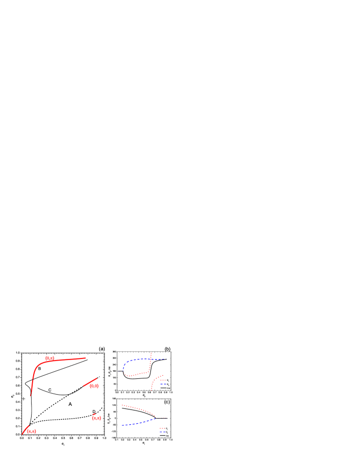
Figure 1: Periodic solutions in the 3:1 MMR. (a) Periodic solution families on the $(e_{1},e_{2})$ plane. The stable symmetrical ACR solutions are thick solid curves, the unstable symmetrical ACR solutions are short-dashed curves, and the thin solid curves indicate the asymmetrical solutions. The value of $(\theta_{1},\Delta\varpi)$ of the symmetrical solutions appear as labels along the curves. We also label different solution families with A, B, C and D. The eccentricities $(e_{1},e_{2})=(0.0197,0.44)$ in Table 1 are indicated by a cross. (b) The variation of the angles $\theta_{1}$ (dotted), $\theta_{2}$ (dashed) and $\Delta\varpi$ (solid) along the solution family A. Note $\Delta\varpi$ begins from $180^{\circ}$ (symmetrical ACR). (c) The same as (b) but for solution family C, where $\Delta\varpi$ reaches at symmetrical value $0^{\circ}$ at the end.

3.1 Periodic solutions in 3:1 MMR

Fig. 1 shows the periodic solutions, both stable and unstable, symmetrical and asymmetical, computed using the mass ratio of the planets 55 Cnc b and 55 Cnc c and assuming coplanar orbits. (For other mass ratios and for details of the method used see [Michtchenko, Beaugé & Ferraz-Mello (2006), Michtchenko et al. (2006)]).

In the real system, if we assume that it evolved from nearly circular orbits through an adiabatical migration, as suggested in many references, the configuration of two planets captured into a 3:1 resonance should be located on or near the family A of periodic solutions shown in Fig. 1(a). In such a migration, the angles $(\theta_{1},\Delta\varpi)$ evolve from the symmetrical $(\pi,\pi)$ values to asymmetrical values. Since each solution family is not connected by stable periodic solutions to other families, there is no reason to expect a system in resonance with orbital configuration far away from the family A. In fact, the eccentricities $(e_{1},e_{2})$ in Table 1 are not on the family A. However, we have found that this configuration could be obtained by a resonance captured from initial eccentric orbits. An example of such kind of resonance trapping is shown in Fig. 2(a). Surely a perturbation happening to a system in the equilibrium periodic solution may also lead to this observed configuration. We just show here another possibility of the resonance formation.

3.2 Jump between solution families

If the disc does not disappear just after the resonance capture happens, the outer planet will continue to migrate inward accompanied by the inner planet locked in the resonance. During such after-capture migration stage, the system will evolve along the solution family A as shown in Fig. 1, provided the migration is “adiabatic”. But if the migration is faster (not adiabatic), as some of our numerical simulations, the solution may jump from a family to another. An example of jump from family A to C is illustrated in Fig. 2(b). Comparing the variations of angles in Fig. 2(c) and Fig. 1(b), (c), it is clear that the jump happens around $t=1.9\times 10^{4}$ yrs. At this moment, if the system goes along family A, the angles $\theta_{1}$ and $\Delta\varpi$ will go up and cross the value $180^{\circ}$ one after another with the increasing eccentricity $e_{2}$. But they fail and turn around following another evolving route, that is, family C. This turnaround is due to some perturbation (in our case it’s the migration itself), and it happens around the critical point where the apsidal difference $\Delta\varpi$ crosses the symmetrical value $180^{\circ}$ in an asymmetical ACR. In fact, the stable region of motion around this critical turning point (on family A with $(e_{1},e_{2})=(0.0423,0.623)$ in Fig. 1(a) ), is very small. Therefore a slight disturbance could drive the system out of the family A.

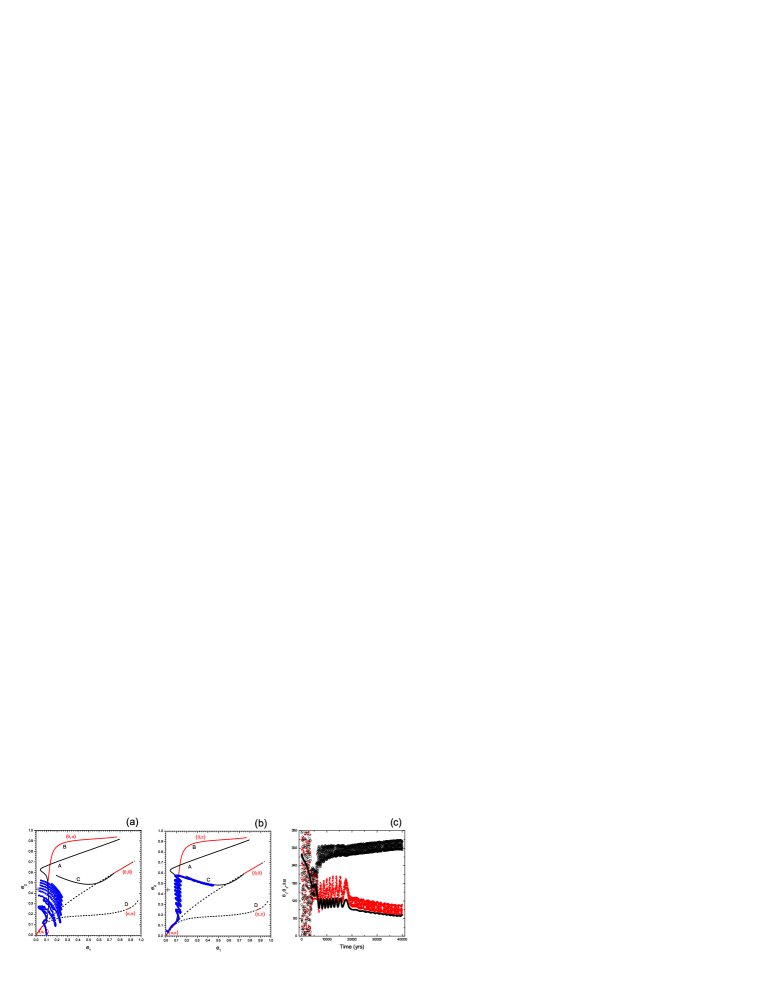
Figure 2: The evolution of orbital configuration in the 3:1 MMR. (a) An example of evolution starting from eccentric initial orbits. The eccentricities in Table 1 can be reached by the solution in this case. Solution families are shown in the same way as in Fig. 1, and the dots indicate the evolution of one run in our numerical simulations. (b) An example of orbital configuration jump from solution family A to family C. (c) The time variations of angles $\theta_{1}$ (small dots), $\theta_{2}$ (open circles) and $\Delta\varpi$ (solid thick curve) for the numerical simulation shown in (b).

The jump from family A to family B has also been observed in our simulations. The angles $\theta_{1}=\theta_{2}=0^{\circ}$ in family B, that is to say, both $\varpi_{1}$ and $\varpi_{2}$ have to adjust to new values in a jump from A to B. On the other hand, as we see from Fig. 1(b),(c) and Fig. 2(c), we need only an adjustment of $\varpi_{1}$ but not $\varpi_{2}$ for a jump from family A to C, since this jump does not affect the $\theta_{2}$. When the jump happens, the inner planet is on a near circular orbit ($e_{1}=0.0423$) while the outer one is on a highly eccentric orbit ($e_{2}=0.623$). As a result, it is much easier to adjust $\varpi_{1}$ than $\varpi_{2}$. This analysis tells why we observe much more A to C jumps than A to B jumps.

These jumps between different solution families make it possible for a resonant system to occupy much larger potential volume in the orbital elements space, increasing the diversity of resonant configuration in extra-solar planetary systems.

4 Conclusions

The 3:1 mean-motion resonance in the 55 Cancri planetary system is far from a necessary result of the differential planetary migration. Our numerical simulations showed that the favourable scenario for the formation of the 3:1 resonance is moderate initial eccentricities ($0.01\sim 0.05$), relatively slower migration ($\tau\sim 10^{5}$ yrs) and suitable eccentricity damping rate ($K\sim 10$). After being captured in the resonance, the system may exhibit some evolutions different from the behaviours in an adiabatic migration, and evolve to some unexpectable orbital configurations. All these put some constraints on the planetary migration and early dynamical evolution in the extra-solar planetary systems.

References

- [Beaugé (2008)] Beaugé, C., 2008, Proceedings of IAUS249, this issue
- [Fischer et al. (2007)] Fischer, D., Marcy, G., Butler, P., Vogt, S., Laughlin, G., Henry, G., Abouav, D., Peek, K., Wright, J., Johnson, J., McCarthy, C. & Isaacson, H. 2007, preprint
- [Kley (2003)] Kley, W. 2003, Cel. Mech. & Dyn. Astron. 87, 85
- [Kley, Peitz & Bryden (2004)] Kley, W., Peitz, J. & Bryden G. 2004, A&A 414, 735
- [Lee & Peale (2002)] Lee, M. & Peale S. 2002, ApJ, 567, 596
- [Marcy et al. (2001)] Marcy, G., Butler, P., Fischer, D., Vogt, S., Lissauer, J., & Rivera, E. 2001, ApJ, 556, 296
- [McArthur et al. (2004)] McArthur, B., Endl, M., Cochran, W., Benedict, F., Fischer, D., Marcy, G., Butler, P., Naef, D., Mayor, M., Queloz, D., Udry, S. & Harrison, T. 2004, ApJ(Letters), 614, L81
- [Michtchenko, Beaugé & Ferraz-Mello (2006)] Michtchenko, T., Beaugé, C. & Ferraz-Mello, S. 2006, Cel. Mech. & Dyn. Astron., 94, 411
- [Nelson & Papaloizou (2002)] Nelson, R. & Papaloizou, J. 2002, MNRAS(Letters), 333 L26
- [Quillen (2006)] Quillen, A. 2006, MNRAS, 365, 1367
- [Ward (1997)] Ward, W. 1997, Icarus, 126, 261
- [Zhou et al. (2004)] Zhou, L.-Y., Lehto, H., Sun, Y.-S. & Zheng, J. 2004, MNRAS, 350, 1495