Two-dimensional elastic turbulence

Abstract

We investigate the effect of polymer additives on a two-dimensional Kolmogorov flow at very low Reynolds numbers by direct numerical simulations of the Oldroyd-B viscoelastic model. We find that above the elastic instability threshold the flow develops the elastic turbulence regime recently observed in experiments. We observe that both the turbulent drag and the Lyapunov exponent increase with Weissenberg, indicating the presence of a disordered, turbulent-like mixing flow. The energy spectrum develops a power-law scaling range with an exponent close to the experimental and theoretical expectations.

One of the most remarkable effects of highly viscous polymer solutions which has been recently observed in experiments is the development of an “elastic turbulence” regime in the limit of strong elasticity GS00 . The flow of polymer solution in this regime displays irregularities typical of turbulent flows (broad range of active scales and growth of flow resistance) even at low velocity and high viscosity, i.e. in the limit of vanishing Reynolds number. As a consequence of turbulent motion at small scales, elastic turbulence has been proposed as an efficient technique for mixing in very low Reynolds flows, such as in microchannel flows GS01 ; BSBGS04 ; AVG05 . Despite its great technological interest, elastic turbulence is still only partially understood from a theoretical point of view. Recent theoretical predictions are based on simplified versions of viscoelastic models and on the analogy with MHD equations BFL01 ; FL03 .

In this letter we investigate the phenomenology of elastic turbulence in direct numerical simulation of polymer solutions in two dimensions. Our main objective is to show that usual viscoelastic models, developed for studying high Reynolds turbulent flows, are able to capture, in the limit of vanishing Reynolds numbers, the main phenomenology of elastic turbulence, i.e. irregular temporal behavior and spatially disordered flow. Despite the important geometrical differences, our numerical results are in remarkable agreement with experimental observations of elastic turbulence: this suggests the possibility to understand elastic turbulence on the basis of known viscoelastic models.

To describe the dynamics of a dilute polymer solutions we adopt the well known linear Oldroyd-B model BCAH87

$$\partial_{t}{\bm{u}}+({\bm{u}}\cdot{\bm{\nabla}}){\bm{u}}=-{\bm{\nabla}p}+\nu{\Delta}{\bm{u}}+\frac{2\eta\,\nu}{\tau}{\bm{\nabla}}\cdot{\bm{\sigma}}+{\bm{f}}$$ (1)

$$\partial_{t}{\bm{\sigma}}+({\bm{u}}\cdot{\bm{\nabla}}){\bm{\sigma}}=({\bm{\nabla}\bm{u}})^{T}\cdot{\bm{\sigma}}+{\bm{\sigma}}\cdot({\bm{\nabla}\bm{u}})-2\frac{({\bm{\sigma}}-{\bm{1}})}{\tau}$$ (2)

where ${\bm{u}}$ is the incompressible velocity field and the symmetric positive definite matrix ${\bm{\sigma}}$ represents the normalized conformation tensor of polymer molecules and ${\bm{1}}$ is the unit tensor. The solvent viscosity is denoted by $\nu$ and $\eta$ is the zero-shear contribution of polymers to the total solution viscosity $\nu_{t}=\nu(1+\eta)$ and is proportional to the polymer concentration. In absence of flow, ${\bm{u}}=0$, polymers relax to the equilibrium configuration and ${\bm{\sigma}}={\bm{1}}$. The trace $\textrm{tr}{\bm{\sigma}}$ is therefore a measure of polymer elongation.

The simplest geometrical setup that will prove useful to study the elastic turbulence regime for viscoelastic flows is the periodic Kolmogorov flow in two dimensions AM60 . With the forcing ${\bm{f}}=(F\cos(y/L),0)$, the system of equations (1-2) has a laminar Kolmogorov fixed point given by

$${\bm{u}}=(U_{0}\cos(y/L),0)$$

(3)

$${\bm{\sigma}}=\left(\begin{array}[]{cc}1+{\tau}^{2}\,{U_{0}^{2}\over 2L^{2}}\sin^{2}{(y/L)}&-{\tau}{U_{0}\over 2L}\sin{(y/L)}\\ -{\tau}{U_{0}\over 2L}\sin{(y/L)}&1\end{array}\right)$$ (6)

with $F=[\nu U_{0}(1+\eta)]/L^{2}$ BCMPV05 . The laminar flow fixes a characteristic scale $L$, velocity $U_{0}$ and time $T=L/U_{0}$. In terms of these variables, we define the Reynolds number as $Re={U_{0}L\over\nu_{t}}$ and the Weissenberg number as $Wi={\tau U_{0}\over L}$. The ratio of these numbers defines the elasticity of the flow $El=Wi/Re$.

It is well known that the Kolmogorov flow displays instability with respect to large-scale perturbations, i.e. with wavelength much larger than $L$. In the Newtonian case, the instability arises at $Re_{c}=\sqrt{2}$ MS61 . At small Reynolds numbers, the presence of polymers can change the stability diagram of laminar flows Larson92 ; GS96 or induce elastic instabilities which are not present in Newtonian fluids LSM90 ; Shaqfeh96 ; BCMPV05 . The Kolmogorov flow is no exception, and recent analytical and numerical investigations have found the complete instability diagram in the $Re$-$Wi$ plane BCMPV05 . For the purpose of the present work, we just have to recall that linear stability analysis shows that for sufficient large values of elasticity, the Kolmogorov flow displays purely elastic instabilities, even at vanishing Reynolds number (see Fig. 1 of BCMPV05 ). We remark that the fact that the original flow has rectilinear streamlines does not exclude the onset of the elastic instability. Above the elastic instability the flow can develop a disordered secondary flow which persists in the limit of vanishing Reynolds number and eventually leads to the elastic turbulence regime GS04 .

The equations of motion (1,2) are integrated by means of a pseudo-spectral method implemented on a two-dimensional grid of size $L_{0}=2\pi$ with periodic boundary conditions at resolution $512^{2}$. Nmerical integrations of viscoelastic models are limited by Hadamard instabilities associated with the loss of positiveness of the conformation tensor SB95 . These instabilities are particularly important at high elasticity and limit the possibility to investigate the elastic turbulent regime by direct implementation of equations (1,2). To overcome this problem, we have implemented an algorithm based on a Cholesky decomposition of the conformation matrix that ensures symmetry and positive definiteness VC03 and allows to reach high elasticities.

Figure 1: Mean power injection normalized with its laminar value $r=P/P_{lam}$ as a function of $Wi=\tau U/L$ for a set of simulations with $\nu=0.769$, $\eta=0.3$, $L=1/4$ and $\tau=4$. The elasticity is $El=64$ and the maximum Reynolds number $Re=Wi/El$ is $Re=0.7$. The line represents the power-law behavior $r\sim Wi^{0.25}$. Inset: amplitude of the Reynolds stress $\Pi_{r}$ ($\times$), polymer stress $\Pi_{p}$ ($+$) and viscous stress $\Pi_{\nu}$ ($*$) nondimensionalized by the total stress amplitude $FL$.

One of the main features of a turbulent-like regime is the growth of the flow resistance to external forcing. This can be quantified as the power needed to maintain a given mean velocity in the turbulent flow. The power injection in (1) is $P=\langle{\bf f}\cdot{\bf u}\rangle$ which, for the laminar flow (3) becomes $P_{lam}=U_{0}^{2}\nu(1+\eta)/(2L^{2})$. A remarkable feature of the Kolmogorov flow is that even in the turbulent regime the mean velocity and conformation tensor are accurately described by sinusoidal profiles BCM05 : $\langle u_{x}\rangle=U\cos(y/L)$, $\langle\sigma_{xy}\rangle=-\Sigma\sin(y/L)$ with different amplitudes with respect to the laminar fixed point. Therefore the reduced average power injection for the turbulent flow is simply

$$r={P\over P_{lam}}={FL^{2}\over\nu(1+\eta)U}$$ (7)

Figure 1 shows the behavior of the power injection as a function of the Weissenberg number $Wi=\tau U/L$. We see that at $Wi\simeq 15$ there is a transition from the laminar regime to a turbulent-like regime in which $r>1$. The growth for the higher values of $Wi$ is compatible with a power law scaling $r\simeq Wi^{0.25}$ which is qualitatively similar with experimental observations BSS07 where an exponent $0.49$ is found. The different exponent observed here can be ascribed to the two-dimensional nature of our flow or to its geometrical property (rectilinear streamlines and absence of material boundaries).

Because the Reynolds number in Fig.1 is always small, and therefore the inertial term in (1) is negligible, it is natural to ask where is the origin of turbulent fluctuations. The momentum budget, in stationary conditions, reads

$$\partial_{y}\Pi_{r}=\partial_{y}(\Pi_{\nu}+\Pi_{p})+f_{x}$$ (8)

where $\Pi_{r}=\langle u_{x}u_{y}\rangle$ is the usual Reynolds stress, $\Pi_{\nu}=\nu\partial_{y}\langle u_{x}\rangle$ the viscous stress and $\Pi_{p}=2\nu\eta\tau^{-1}\langle\sigma_{xy}\rangle$ is the stress induced by polymers. The numerical observation that also the Reynolds stress is well described by a monochromatic profile, $\langle u_{x}u_{y}\rangle=U_{2}\sin(y/L)$, allows us to write the momentum budget for the amplitudes as $FL=U_{2}+\nu U/L+(2\nu\eta/\tau)\Sigma$. The inset of Fig.1 shows the different contributions (normalized with the total stress) as a function of $Wi$. In the laminar regime ($Wi\to 0$) $U_{2}=0$ and from (3) one has $\Pi_{p}/\Pi_{\nu}=\eta$. Above the transition to elastic turbulence, the polymer stress starts growing and reaches a value close to the viscous stress at the present maximum Weissenberg number. We remark that we observe no indication of saturation and therefore we may expect $\Pi_{p}$ to become the dominant term at larger values of $Wi$. The contribution of the Reynolds stress always remains smaller than $10^{-2}$, confirming the irrelevance of inertial terms. This is the hallmark of elastic turbulence where elastic stress has the role played by the Reynolds stress in usual turbulence.

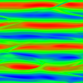
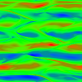
Figure 2: (color online) Snapshot of vorticity field at $Wi=22$ (left) and $Wi=45$ (right). The flow is forced with a Kolmogorov forcing $f_{x}=Fcos(y/L)$ with $L=1/4$.

In order to get more insight in the elastic turbulence flow, in Fig. 2 we show two snapshots of the two-dimensional vorticity field at two different $Wi$. The first snapshot is taken at $Wi=22$, slightly above the elastic instability threshold. The flow in this regime is still not turbulent and a secondary flow in the form of thin filaments is clearly observable. These small scale filaments, moving along the $x$ direction, are elastic waves, reminiscent of the Alfven waves propagating in presence of a large scale magnetic field in plasma. Indeed, the possibility of observe elastic waves in polymer solution was theoretically predicted within a simplified uniaxial elastic model FL03 which has strong formal analogies with MHD equations, but they were never observed before.

At higher values of elasticity the vorticity pattern becomes progressively more irregular with chaotic motion of filaments. At $Wi=45$ we observe a highly irregular pattern in which the underlying basic flow is hardly distinguishable. This is the regime of elastic turbulence in which the flow develops active modes at all the scales. Fig. 3 shows the power spectrum of velocity fluctuations averaged over several configurations like the one shown in Fig. 2. A power-law behavior $E(k)\simeq k^{-\alpha}$ is clearly observable with a spectral exponent $\alpha$ larger than $3$. Again, this is in quantitative agreement with what observed in laboratory experiments GS00 and with the theoretical predictions based on the uniaxial model FL03 .

Figure 3: Velocity fluctuation spectra at $Wi=26$ (squares) and $Wi=45$ (circles). The line represents the power-law behavior $k^{-3.8}$.

One of the most promising applications of elastic turbulence is efficient mixing at very low Reynolds number. This is an issue of paramount importance in many industrial problems, namely in microfluidic applications. Indeed, laboratory experiments in curvilinear channels have demonstrated that very viscous polymer solutions in the elastic turbulence regime are very efficient for small scale mixing GS01 . Mixing efficiency of polymer solutions has been studied in various setups, including microchannels BSBGS04 and two-dimensional magnetically driven flows AVG05 . Because in the elastic turbulent regime the flow is smooth (i.e. the energy spectrum is steeper that $k^{-3}$) a suitable characterization of mixing is given in terms of Lagrangian Lyapunov exponent $\lambda$ PV87 . This is defined as the mean rate of separation of two infinitesimally close particles transported by the flow and, in the present case, is related to the polymer stretching rate BCM03 .

Figure 4: Lagrangian Lyapunov exponent as a function of the Weissenberg number. Inset: Cramer function for three different Weissenberg numbers: $Wi=12$ (solid line), $Wi=21$ (dashed line) and $Wi=53$ (dotted line).

Figure 4 shows the behavior of the Lyapunov exponent as a function of $Wi$ at fixed $Re=1$. We observe that, above $Wi=10$, $\lambda$ grows and saturates at values $\approx 2/\tau$ for $Wi$ larger than $60$. We remark that this behavior is opposite to the one observed in the case of high Reynolds numbers viscoelastic flows where the injection of polymers reduces the degree of chaoticity by lowering $\lambda$ below $1/\tau$ BCM03 .

In the inset of Fig. 4 we plot the Cramer function $G(\gamma)$ which is defined from the probability density functions of finite-time Lyapunov exponents $P_{t}(\gamma)\sim\exp(-tG(\gamma))$ PV87 . As it is evident, increasing $Wi$ not only the degree of mean chaoticity increases, but also fluctuations becomes larger, in particular the distribution of $\gamma$ becomes asymmetric with a larger relative probability of positive fluctuations. It is remarkable that the same qualitative behavior is observed in the case of high-Reynolds Newtonian turbulence, where the distribution of Lyapunov fluctuations becomes more asymmetric with increasing $Re$ BBBCMT06 . This suggests that in elastic turbulence elasticity (i.e. $Wi$) plays a similar role as non-linearity (i.e. $Re$) in ordinary hydrodynamic turbulence.

Finally, we have investigated the dependence of polymer statistics on the Weissenberg number. In Figure 5 we show the average squared polymer elongation $\langle\mathrm{tr}{\bm{\sigma}}\rangle$ integrated over the flow volume and the amplitude of cross stress $\Sigma$. At small $Wi$ these follow the laminar behavior, i.e. $2+Wi^{2}/4$ and $Wi/2$, respectively. At the onset of elastic turbulence the cross polymer stress $\Sigma$ grows faster than linearly in $Wi$, as already shown in Figure 1, and eventually appears to approach a power-law behavior with a slope close to $1.5$. On the contrary, the squared polymer elongation in elastic turbulence grows more slowly than its laminar value. This is probably due to the loss of coherence in stretching experienced in the turbulent flow. At large $Wi$ an asymptotic behavior $\sim Wi^{1.5}$ appears to set in for $\mathrm{tr}{\bm{\sigma}}$ as well and the ratio $\langle tr{\bm{\sigma}}\rangle/\Sigma$ becomes constant.

Figure 5: Average polymer elongation $\langle tr{\bm{\sigma}}\rangle$ (open circles) and polymer stress amplitude $\Sigma$ (filled circles) as a function of $Wi$. Lines represent the laminar behaviors $2+Wi^{2}/4$ (continuous) and $Wi/2$ (dotted).

Summarizing, we have shown that elastic turbulence can be successfully reproduced numerically with the aid of a widely known viscoelastic model of polymer solutions (the Oldroyd-B model) and a simple geometrical setup (the two-dimensional Kolmogorov flow). Most observed features have a strong qualitative resemblance with experimental results. Quantitative differences exist, however, and may be traced back to the two-dimensional or to the boundaryless nature of our toy flow, or both. In this context it would prove extremely useful to perform numerical simulations in more realistic geometries and dimensionality to ascertain the origin of such differences.

We thank V. Steinberg for valuable discussions. This work was carried out under the auspices of the National Nuclear Security Administration of the U.S. Department of Energy at Los Alamos National Laboratory under Contract No. DE-AC52-06NA25396. SB acknowledges the support of TEKES-2007 ”Multimodel” project.

References

- (1) A. Groisman and V. Steinberg, Nature 405, 53 (2000).
- (2) A. Groisman and V. Steinberg, Nature 410, 905 (2001).
- (3) T. Burghelea, E. Segre, I. Bar-Joseph, A. Groisman and V. Steinberg, Phys. Rev. E 69, 066305 (2004).
- (4) P.E. Arratia, G.A. Voth and J.P. Gollub, Phys. Fluids 17 053102 (2005).
- (5) E. Balkovsky, A. Fouxon and V. Lebedev, Phys. Rev. E 64, 056301 (2001).
- (6) A. Fouxon and V. Lebedev, Phys. Fluids 15, 2060 (2003).
- (7) R.B. Bird, C.F. Curtiss, R.C. Armstrong, and O. Hassager, Dynamics of polymeric fluids Vol.2, Wiley, New York (1987).
- (8) V.I. Arnold and L. Meshalkin, Uspekhi Mat. Nauk 15, 247 (1960).
- (9) G. Boffetta, A. Celani, A. Mazzino, A. Puliafito and M. Vergassola, J. Fluid Mech. 523, 161 (2005).
- (10) L. Meshalkin and Y.G. Sinai J. Appl. Math. Mech. 25, 1700 (1961).
- (11) R.G. Larson, Rheol. Acta 31, 213 (1992).
- (12) A. Groisman and V. Steinberg, Phys. Rev. Lett. 77, 1480 (1996).
- (13) R.G. Larson, E.S.G. Shaqfeh and S.J. Muller, J. Fluid Mech. 218, 573 (1990).
- (14) E.S.G. Shaqfeh, Annu. Rev. Fluid Mech. 28, 129 (1999).
- (15) A. Groisman and V. Steinberg, New J. Phys. 6, 29 (2004).
- (16) R. Sureshkumar and A.N. Beris, J. Non-Newtonian Fluid Mech. 60, 53 (1995).
- (17) T. Vaithianathan and L.R. Collins, J. Comp. Phys. 187, 1 (2003).
- (18) G. Boffetta, A. Celani and A. Mazzino, Phys. Rev. E 71, 036307 (2005).
- (19) T. Burghelea, E. Segre and V. Steinberg, Phys. Fluids 19, 053104 (2007).
- (20) G. Paladin and A. Vulpiani, Phys. Rep. 156, 147 (1987).
- (21) G. Boffetta, A. Celani and S. Musacchio, Phys. Rev. Lett. 91, 034501 (2003).
- (22) J. Bec, L. Biferale, G. Boffetta, M. Cencini, S. Musacchio and F. Toschi, Phys. Fluids 18, 091702 (2006).