How winding is the coast of Britain ? Conformal invariance of rocky shorelines

Abstract

We show that rocky shorelines with fractal dimension $4/3$ are conformally invariant curves by measuring the statistics of their winding angles from global high-resolution data. Such coastlines are thus statistically equivalent to the outer boundary of the random walk and of percolation clusters. A simple model of coastal erosion gives an explanation for these results. Conformal invariance allows also to predict the highly intermittent spatial distribution of the flux of pollutant diffusing ashore.

I Introduction

Forty years after Mandelbrot’s seminal paper [Mandelbrot, 1967] where the concept of fractional dimension was introduced, there is a compelling evidence of the fractal nature of many geographical phenomena, including the shaping of shorelines [Goodchild and Mark, 1987]. Statistically self-similar curves are characterized by their fractal exponent $D$. If we select two points on the curve and measure their distance $L$ along the curve (e.g. by walking a divider of given width) on average this will be proportional to their Euclidean distance $R$ to the power $D$, i.e. $L\sim R^{D}$, where $D$ can take values between $1$ and $2$. Such curves are widespread in nature, and often enjoy a much richer symmetry than mere global scale invariance. This is the case of conformally invariant curves, whose statistics is covariant with respect to local scale transformations, i.e. coordinate changes that preserve the relative angle between two infinitesimal segments. Conformal invariance is a pervasive feature of two-dimensional physics, from string theory and quantum gravity to the statistical mechanics of condensed matter and fluid turbulence [Polyakov, 1970; Belavin et al., 1984; Schramm, 2006; Bernard et al., 2006, 2007]. A remarkable consequence of conformal invariance is the high degree of symmetry that often allows to make substantial analytical progress [Cardy, 2005; Bauer and Bernard, 2006]. Among the many characteristic features that make conformally invariant curves peculiar within the class of self-similar ones, the former are also distinguished by the special statistics of the winding angle about a point belonging to the curve itself (see Fig. 1b). The probability distribution of the winding angle is Gaussian, and therefore specified only by its mean (that is zero, i.e. curves do not have a preferred winding direction, or chirality), and its variance, that increases proportionally to the logarithm of the distance from the reference point with a proportionality constant which depends on the fractal dimension. This provides a simple and useful diagnostics for conformal invariance of curves extracted from experimental or numerical data.

Here we show that rocky shorelines display a Gaussian distribution of winding angles with a logarithmic dependence of the variance as expected for conformally invariant curves with the correct numerical prefactor. We use conformal invariance to predict the statistics of the flux of pollutant diffusing over shorelines, which characterized by a strongly intermittent spatial distribution which can vary dramatically between locations just a few hundred meters apart (see for instance Fig. 1 of Peterson et al. [2003] about the Exxon-Valdez oil spill).

II Statistical analysis of rocky shoreline

Since the famous paper of Mandelbrot [1967], the west coast of Britain has become the paradigmatical example of fractal shoreline. In Figure 1 we show a satellite image of a portion of the western coast of Scotland along with its digitized shoreline, that is a polygonal approximation to the real coastline. It is also displayed in a double logarithmic plot the fraction of pairs of vertices of the polygon that lie within a ball of diameter $R$: the slope of this curve is the correlation dimension [Grassberger and Procaccia, 1983], that is very close to $4/3$ in this case.

The shoreline shown in Fig. 1 is one example of the curves extracted from the high-resolution, self-consistent GSHHS database [Wessel and Smith, 1996]. The complete database covers the world shoreline which has been partitioned into $11503$ segments of length $\approx 200$ km with a resolution of about $200$ m. The computation of fractal dimension (as in Fig. 1) for each segment, gives different values of $D$ that depend on the geomorphological processes at work in that particular geographical area. We observe a fractal dimension close to $1$ for sedimentary shores while for rocky coasts it is about $1.3$ or larger. The overall most probable value is found to be $D\simeq 1.2$. Within this large sample, we have selected the $1146$ shorelines which present a correlation dimension close to $D=4/3$ (with a tolerance of $5\%$). The capacity dimension for such curves, computed by a box-counting algorithm, yields a value consistent with the correlation dimension, pointing to the conclusion that these are truly fractal curves and not multifractals [Grassberger and Procaccia, 1983].

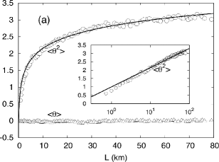
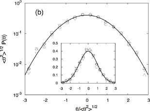
Figure 2: Winding angle statistics. Panel (a) shows the mean and the variance of the winding angle as a function of the length of the shoreline between points $P$ and $Q$. (see Fig. 1). The line is the law $\langle\theta^{2}\rangle=a+\frac{2(D-1)}{D}\ln L$ with $D=4/3$ and $a=0.98$. In the inset, the variance in semilogarithmic coordinates. In panel (b) is shown the probability density function of the winding angle at lengths $L=5,10,20$ km rescaled by the respective standard deviation and compared to the standard Gaussian density, in semilogarithmic (main frame) and in linear coordinates (inset).

The statistics of winding angles for rocky coastlines is shown in Fig. 2. The winding angle $\theta$ is defined as the angle between the line joining two points separated by a length $L$ along the curve and the local tangent in the reference point, measured counterclockwise in $rad$ (see Fig. 1b). Because our curves do not have a preferred direction, the mean winding angle $\langle\theta\rangle$ is very close to zero while the variance is found to grow with $L$ according to the logarithmic law predicted for conformal invariant curves [Duplantier and Saleur, 1988; Duplantier and Binder, 2002; Wieland and Wilson, 2003]

$$\langle\theta^{2}\rangle=a+{2(D-1)\over D}\ln L$$ (1)

Here $a$ is a constant that depends on the details of the definitions and whose actual value is irrelevant. The numerical evaluation of the coefficient in (1) gives $D\simeq 1.33$, i.e. very close to the direct measure of $D$. Figure 2b shows that the probability density function (pdf) of $\theta$ is very close to a Gaussian distribution for different separations in the logarithmic range. Winding angle statistics have been computed using different reference points located along the curve: we have found no detectable dependence on this choice.

Values of the fractional dimension other than $4/3$ (e.g. $D=1.2$ and $D=1.5$) fail to give such an impressive agreement with the prediction for conformally invariant curves, in the sense that the prefactor differs significantly from the value predicted by (1). An explanation for the peculiarity of this value of $D$ is provided by a simple model, introduced by Sapoval et al. [2004], of mechanical erosion of rocky coasts. Of course, the real properties of rocky coast morphology are the result of several mechanisms acting on various space-time scales [Carter and Woodroffe, 1994] and are beyond the scope of this simple modeling. The basic ingredients of this model are two: (i) the mechanical resistance of rocks to erosive processes, essentially determined by their structure, composition and by the slow corrosion process due to chemical agents, is assumed to have a typical scale of variation of the order of hundreds of meters and to be essentially uncorrelated on larger distances; (ii) rocks that are more exposed to the action of waves have a larger propensity to be fragmented by mechanical erosion: for instance, an isthmus will be eroded more rapidly than the shoreline within a gulf.

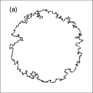
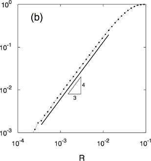
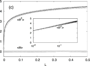
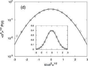
Figure 3: Artificial shorelines. In panel (a) one example of a coast generated by the model of wave erosion described in the text. The simulation has been done on a square grid with $8000^{2}$ collocation points. The number of realizations is $800$. Panel (b) shows the correlation dimension. The unit for $R$ and $L$ is the simulation box size. A fit in the range of $R$ between $5\cdot 10^{-4}$ and $0.1$ yields $D=1.32\pm 0.02$. Panels (c) and (d) show the winding angle statistics as in Fig. 2 compared to the theoretical expectations.

This model can be implemented on a two-dimensional lattice where the sites represent regions of land or sea of dimensions about a hundred meters. To every point on the land is assigned a number that measures the resistance of the rock to erosion. Then, if the resistance of a land site adjacent to the sea falls below a given threshold, it will be eroded, and thus transform into a sea site. Subsequently, the resistance values for land sites along the shoreline are updated depending on the local conformation of the coast [Sapoval et al., 2004]. This procedure is iterated until no further updates are necessary and a stationary artificial shoreline is obtained (see Fig. 3a). The similarities of this model with the well-known problem of percolation [Stauffer and Aharony, 1991] are evident, as already pointed out in Sapoval et al. [2004]. Indeed, in presence of rule (i) alone the islands generated by the algorithm would be statistically equivalent to percolation clusters — except for the inner “lakes” present in the latter case — and thus display a fractal dimension $7/4$. However, rule (ii) prevents the formation of deep gulfs and peninsulae with narrow isthmi, therefore reducing the shoreline to the outer boundary of percolation clusters that is known to have fractal dimension $4/3$ [Grossman and Aharony, 1986; Saleur and Duplantier, 1987]. Further refinements of the model, including damping of sea-waves and slow erosive processes do not modify the main features described above. As a consequence of the statistical equivalence between the artificial shoreline and the external frontier of percolation clusters, the former inherits the known conformal invariance of the latter. In Figure 3 we show the numerical results for the artificial shorelines generated by the model, which confirm the theoretical expectations.

III Intermittency of diffusing pollutants

By virtue of the rich symmetry underlying conformal invariance, many interesting results can be obtained analytically. As a remarkable example we consider here the evaluation of the flux of pollutant diffusing ashore from a source located in the sea. Transport and mixing of tracers is a complex issue of paramount importance from microscopic to planetary scales [Ottino, 1989]. At the simplest level of description dispersion is modeled as pure diffusion. In the present case, this may be justified by estimates of the horizontal eddy-diffusivity in the ocean that yield a ratio about $0.1$ to $1$ between mean currents and velocity fluctuations over scales of a hundred kilometers [Marshall et al., 2006].

Pollutant concentration $c$ is therefore assumed to be given by the solution of the Laplace equation $\Delta c=0$ with a pointwise source in the ocean and absorbing boundary conditions on the coastline ($c=0$). This problem can be solved with the aid of conformal transformations by mapping the region of interest (i.e. a region of sea bounded by the shoreline) into an infinite strip, solving the Laplace problem in the new domain (now a trivial task), and mapping the solution back to the initial region.

The upshot of the conformally invariant nature of the shoreline is that techniques borrowed from theoretical physics enable to compute analytically the pollutant flux distribution $\phi=\partial c/\partial n$ at the boundary [Duplantier, 2000; Duplantier and Binder, 2002; Bettelheim et al., 2005]. The main result is that the probability of observing a flux $\phi$ of intensity $\phi_{0}(R/R_{0})^{\alpha}$ — where $\phi_{0}$ is the rate of emission by the source, $R$ the size of the region where the flux is computed, and $R_{0}$ the distance of the source from the coast — is proportional to $(R/R_{0})^{-f(\alpha)}$ with $f(\alpha)=\alpha+\frac{(2D-1)^{2}}{4(D-1)}\left[1-\alpha^{2}/(2\alpha-1)\right]$, for $R\ll R_{0}$. Small values of the flux correspond to large values of $\alpha$, whereas the largest ones take place for $\alpha\searrow 1/2$. This can be understood by means of the geometrical interpretation of the variable $\alpha$ [Duplantier, 2000]. Indeed, let us recall that the flux inside a wedge of opening angle $\theta$ scales exactly as $R^{\pi/\theta}$. The result above can thus be interpreted as if the shoreline was made of a random collection of wedges of size $\sim R$ and opening angles $\theta$ with probability $\sim R^{-f(\pi/\theta)}$. Large $\alpha$ and small fluxes are equivalent to small $\theta$, i.e. deep fjords in the shoreline. On the opposite, as $\alpha$ reaches the minimum value $1/2$, the flux attains its maximum value $\sim\phi_{0}(R/R_{0})^{1/2}$ corresponding to $\theta=2\pi$, that is a needle-like cape. The average flux $\langle\phi\rangle$ is exactly $\phi_{0}$. By means of a variable change from $\alpha$ to $\phi$ it is possible to derive the exact probability density for the flux. Besides the exact form, it is interesting to notice that for $\phi\ll\phi_{0}$ the probability of observing a value $\phi$ of the flux scales as a power law:

$$p(\phi)\sim\phi^{-2+\frac{(2D-1)^{2}}{8(D-1)}}$$ (2)

This power-law dependence is a reflection of the strongly intermittent character of flux fluctuations. In Figure 4 we show the flux of pollutant emitted for a source located $40$ km offshore the coastline of Fig 1, together with its probability density. This closely follows the theoretical predictions for small fluxes over a range of several decades. Note that similar arguments hold for the longitudinal flux of pollutant diffusing along the shoreline under reflecting boundary conditions.

In conclusion, we have demonstrated that world coastlines with dimension $D\simeq 4/3$ are conformally invariant curves by measuring their winding angle statistics. The distinguishing feature of such random curves is their high degree of symmetry which enables to compute analytically many statistical properties. We have focused our attention on the flux of pollutant diffusing toward the shoreline, however many other interesting results could be relevant to geophysical applications. For instance, an archipelago of conformally invariant islands (loops) would display a power law distribution $A^{-1}$ of the number of islands of area larger than $A$ with a known prefactor. These would be also characterized by a ratio between the average area and the average squared radius equal to $\pi D/(2D-1)$. All these properties, and many others, are also shared by self-avoiding walks (polygons), i.e. closed random walks that never hit themselves. These have been conjectured to be conformally invariant curves with dimension $4/3$ via the equivalence with stochastic Loewner evolution curves SLE_8/3 (see Lawler et al. [2004] for a review). Remarkably enough, self-avoiding walks were introduced by Mandelbrot as well, when he conjectured the (now proven) equivalence between them and the external frontier of two-dimensional Brownian motion. Today, in view of our results, all these curves reveal their unexpected and intimate connection with the brilliant intuition by Richardson and Mandelbrot about the fractal nature of world coastlines.

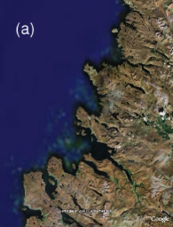
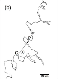
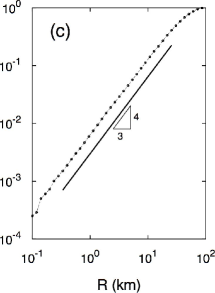
Figure 1: The west coast of Scotland: an example of the $1146$ shorelines that have been searched for conformal invariance. Panel (a) shows the satellite image of the geographical area, centered around the point $58^{\circ}05^{\prime}$N, $5^{\circ}21^{\prime}$W. In Panel (b) is shown the GSHHS polygonal approximation of the shoreline with resolution $\approx 200$ m together with an example of winding angle between points $Q$ and $P$. Panel (c) shows the fraction of pairs of points of the curve (b) lying at a distance smaller than $R$. The logarithmic slope of the curve is the fractal correlation dimension. A least-squares fit for the data over the range from $300$ m to $20$ km gives an exponent $1.30\pm 0.04$. Also shown for comparison a straight line of slope $4/3$.

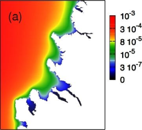
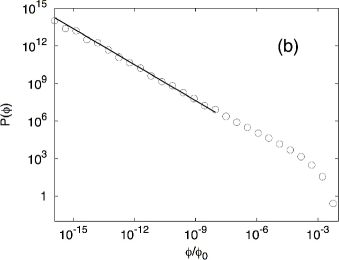
Figure 4: Flux of diffusing pollutant. In panel (a) is shown the contour plot of the pollutant concentration in the domain bounded by the shoreline of Fig. 1. Panel (b) shows the probability density of flux computed along the present shoreline, compared with the theoretical expectation (2) for the left tail.

- (1) Bauer, M., and D. Bernard (2006), 2D growth processes: SLE and Loewner chains, Phys. Rep., 432, 115.
- (2) Belavin, A.A., A.M. Polyakov, and A.A. Zamolodchikov (1985), Conformal field theory, Nucl. Phys. B, 241, 333.
- (3) Bernard, D., G. Boffetta, A. Celani, and G. Falkovich (2006), Conformal invariance in two-dimensional turbulence, Nature Physics, 2, 124.
- (4) Bernard, D., G. Boffetta, A. Celani, and G. Falkovich, Inverse turbulent cascades and conformally invariant curves, Phys. Rev. Lett., 98, 024501.
- (5) Bettelheim, E., I. Rushkin, I.A. Gruzberg, and P. Wiegmann (2005), Harmonic Measure of Critical Curves, Phys. Rev. Lett., 95, 170602.
- (6) Cardy, J. (2005), SLE for theoretical physicists, Ann. Phys., 318, 81.
- (7) Carter, R.W.G., and C.D. Woodroffe (1994), Coastal evolution. Late Quaternary shoreline morphodynamics, Cambridge Univ. Press, Cambridge
- (8) Duplantier, B. (2000), Conformally Invariant Fractals and Potential Theory, Phys. Rev. Lett., 84, 1363.
- (9) Duplantier, B., and I. A. Binder (2002), Harmonic Measure and Winding of Conformally Invariant Curves, Phys. Rev. Lett., 89, 264101.
- (10) Duplantier, B., and H. Saleur (1988), Winding-Angle Distributions of Two-Dimensional Self-Avoiding Walks from Conformal Invariance, Phys. Rev. Lett., 60, 2343.
- (11) Goodchild, M.F., and D.M. Mark (1987), The fractal nature of geographic phenomena, Annals of the Association of American Geographers, 77, 265.
- (12) Grassberger, P., and I. Procaccia (1983), Measuring the strangeness of strange attractors, Physica D, 9, 189.
- (13) Grossman, T., and A. Aharony (1986), Structure and perimeters of percolation clusters, J. Phys. A, 19, L745.
- (14) Lawler, G.F., O. Schramm, and W. Werner (2004), On the scaling limit of planar self-avoiding walk, Proc. Sympos. Pure Math., 72, 339.
- (15) Mandelbrot, B. (1967), How long is the coast of Britain ? Statistical self-similarity and fractional dimension, Science, 156, 636.
- (16) Marshall, J., E. Shuckburgh, H. Jones, and C. Hill (2006), Estimates and Implications of Surface Eddy Diffusivity in the Southern Ocean Derived from Tracer Transport, J. Phys. Oceanog., 36, 1806.
- (17) Ottino, J.M. (1989), The kinematics of mixing: stretching, chaos, and transport, Cambridge University Press.
- (18) Peterson, C.H. et al (2003), Long-Term Ecosystem Response to the Exxon Valdez Oil Spill, Science, 302, 2082.
- (19) Polyakov, A.M. (1970), Conformal symmetry of critical fluctuations, JETP Lett., 12, 381.
- (20) Saleur, H., and B. Duplantier (1987), Exact Determination of the Percolation Hull Exponent in Two Dimensions, Phys. Rev. Lett., 58, 2325.
- (21) Sapoval, B., A. Baldassarri, and A. Gabrielli (2004), Self-Stabilized Fractality of Seacoasts through Damped Erosion Phys. Rev. Lett., 93, 098501.
- (22) Schramm, O. (2006), Conformally invariant scaling limits (an overview and a collection of problems), math.PR/0602151.
- (23) Stauffer, D., and A. Aharony (1991), Introduction to Percolation Theory Taylor and Francis, London.
- (24) Wessel, P., and W.H.F. Smith, (1996), A Global Self-consistent, Hierarchical, High-resolution Shoreline Database, J. Geophys. Res., 101, B4, 8741.
- (25) Wieland, B., and D. B. Wilson (2003), Winding angle variance of Fortuin-Kasteleyn contours, Phys. Rev. E, 68, 056101.