Wavefunction considerations for the central spin decoherence problem in a nuclear spin bath

Abstract

Decoherence of a localized electron spin in a solid state material (the “central spin” problem) at low temperature is believed to be dominated by interactions with nuclear spins in the lattice. This decoherence is partially suppressed through the application of a large magnetic field that splits the energy levels of the electron spin and prevents depolarization. However, the dephasing decoherence resulting from a dynamical nuclear spin bath cannot be removed in this way. Fluctuations of the nuclear field lead to an uncertainty of the electron’s precessional frequency in a process known as spectral diffusion. This paper considers the effect of the electron’s wavefunction shape on spectral diffusion and provides wavefunction dependent decoherence time formulas for a free induction decay as well as spin echoes and concatenated dynamical decoupling schemes for enhancing coherence. We also discuss a dephasing of a qubit encoded in singlet-triplet states of a double quantum dot. A central theoretical result of this work is the development of a continuum approximation for the spectral diffusion problem which we have applied to GaAs and InAs materials specifically.

I Introduction

Understanding quantum decoherence is a fundamental subject of interest in modern physics. In this work, we theoretically study the issue of quantum decoherence for the problem of one localized electron spin in a solid state nuclear spin environment, where the electron spin eventually loses its quantum phase memory (i.e., dephases) due to its interaction with the surrounding nuclear spin bath. This is often called “central spin” decoherence in a spin bath, with the localized electron spin being the central spin and the surrounding nuclear spin environment being the spin bath. This particular problem is important in the context of quantum information processing and quantum computation using localized electron spins as qubits, and as such, we concentrate on a few systems of interest in solid state quantum computation architectures, namely, Si:P donor electron spin qubits and GaAs and InAs quantum dot electron spin qubits, all of which have considerable recent experimentaltyryshkin ; abe ; petta05 ; Delft ; modeLock and theoreticaldesousa03b ; Basel ; witzelHahnShort ; yaoHahn ; deng ; witzelHahnLong ; witzelCPMG ; yaoCDD ; yaoCDDlong ; witzelCDD interest. The theory we develop is, however, applicable to the general situation of the quantum dephasing of a single localized electron spin in solids due to the environmental influence of the slowly fluctuating nuclear spin bath consisting of many millions of surrounding nuclear spins mutually flip-flopping due to their magnetic dipolar coupling.

The issue of specific interest in this paper, as the title of this paper suggests, is how the detailed form of the confinement for the localized electron in the solid (e.g., the exponentially confined hydrogenic confinement for the localized P donor electron state in Si or the Gaussian-type simple harmonic oscillator confinement for the localized electron in the GaAs/InAs quantum dot) could have qualitative influence on its nuclear induced spin dephasing. This subtle (but potentially significant) dependence of electron spin dephasing on the nature of the electron localization has recently been emphasized in the discoveryUDD that a particular type of dynamical decoupling (DD) sequenceUhrigSequence can be ideal in restoring quantum coherence in the GaAs quantum dot system, but not particularly effective in the Si:P system, which can be traced back to the Gaussian versus the exponential wavefunction localization in the two systems, leading to the validity or the lack thereof of a particular time perturbation expansion as discussed in depth in this work. Thus, a detailed investigation of the effect of the localized electron wavefunction on the nuclear induced electron spin dephasing problem is both important and timely in view of the intense current activity in fault-tolerant quantum computation using spin qubits in semiconductors.

It is important in the context of studying electron spin decoherence to distinguish among three different spin relaxation or decoherence times, $T_{1}$, $T_{2}^{*}$, and $T_{2}$, which are discussed in the literature. (We should mention right at the outset that our work is focused entirely on $T_{2}$, sometimes also denoted $T_{M}$ or spin memory time. $T_{2}$ is variously called spin decoherence time, spin dephasing time, transverse spin relaxation time, spin-spin relaxation time, and spin memory time in the literature.) The spin relaxation time $T_{1}$, also often called the longitudinal spin relaxation time or the energy relaxation time, is connected with the spin flip process which, in the presence of an externally applied magnetic field (the case of interest to us in this work), necessarily requires phonons (and spin-orbit coupling) to carry away the electron spin Zeeman energy, which is 3 orders of magnitude larger than the nuclear spin Zeeman energy. This $T_{1}$-relaxation process can be made arbitrarily long by lowering the lattice temperature so that phonons are simply not available to provide the energy conservation. At the low ($\sim 100~{}\mbox{mK}$ or lower) temperatures of interest to us in the quantum computing context, the relevant $T_{1}$ times are very long ($T_{1}>100~{}\mbox{ms}\gg T_{2}$) and are unimportant for our consideration. The $T_{2}^{*}$ time is the relevant decoherence time in the presence of substantial inhomogeneous broadening as, for example, in ensemble measurements over many electron spin qubits with varying (i.e., inhomogeneous) nuclear spin environments. In the context of single spin qubits, i.e. involving a single electron spin, the $T_{2}^{*}$ decoherence sets in due to the requisite time averaging which, due to ergodicity, becomes equivalent to the spatial inhomogeneity of the varying nuclear spin environments of many electron spins. Thus, $T_{2}^{*}$ is measured either in a measurement over an ensemble of localized spins with the associated spatial averaging or in a time-averaged measurement for a single spin over many runs. A spin echo (or Hahn spin echo) measurement gets rid of the inhomogeneous broadening and characterizes $T_{2}$, the pure dephasing time of a single spin (typically for the systems of our interest $T_{2}^{*}\lesssim T_{2}/1000$ and $T_{2}<T_{1}/1000$), which is what we theoretically study in this work. A closely related, but by no means identical, definition of $T_{2}$ comes from considering the free induction decay (FID) of a single spin in a single-shot measurement without involving either spatial averaging over many spin qubits or temporal averaging over many runs. Alternatively, FID is observed in a homogeneous ensemble. We will call such a FID dephasing time $T_{I}~{}(\lesssim T_{2})$ to distinguish it from the spin echo dephasing time $T_{2}$.

The above discussion of $T_{1}$, $T_{2}^{*}$, $T_{2}$, and $T_{I}$ illustrates the considerable semantic danger of discussing “spin decoherence” because, depending on the context, the “spin decoherence time” for the same system could vary by many orders of magnitude (i.e., $T_{1}\gg T_{2}\gtrsim T_{I}\gg T_{2}^{*}$, etc.). To avoid such confusion, we emphasize that, in our opinion, the only sensible way of discussing spin decoherence is by considering specific experimental contexts. Our definition of $T_{2}$ is thus the decoherence time measured in a Hahn spin echo experiment. The only license we take with our definition of $T_{2}$ is that we continue using $T_{2}$ as the notation for spin decoherenc time even in situations where the spin coherence has been extended far beyond the Hahn spin echo time by using multiple pulse sequences [Carr-Purcell-Meiboom-Gill (CPMG), concatenated dynamical decoupling (CDD), etc.] much more complex than the single $\pi$-pulse Hahn sequence. For us, therefore, $T_{2}$ is the spin decoherence time as measured in an echo-type pulse sequence measurement, which could be a simple $\pi$-pulse spin echo or more complex pulse sequences meant to prolong spin memory beyond the spin echo refocusing.

Finally, we point out an additional important complication, often erroneously neglected in the literature, associated with discussing spin decoherence in terms of a single decoherence time parameter, $T_{\mbox{\tiny Coh}}$ (e.g., $T_{1}$ or $T_{2}$ or $T_{2}^{*}$ or $T_{I}$, etc.). Such a description assumes, by definition, that the quantum memory (i.e., some precisely defined quantum amplitude or probability) falls off in a simple exponential manner with time, i.e., $\exp{(-t/T_{\mbox{\tiny Coh}})}$ or $\exp{(-[t/T_{\mbox{\tiny Coh}}]^{n})}$, where $n$ is a constant, so that a single decoherence time $T_{\mbox{\tiny Coh}}$ can completely parametrize the nature of decoherence. This is, however, not always the case, and the detailed functional dependence of quantum coherence on time almost always changes with $t$ in a complex manner, ruling out any simple single-parameter characterization of spin decoherence. To be consistent with the standard literature, we often discuss or describe our results by a single $T_{2}$, but we simply define $T_{2}$ as the time it takes for the quantum memory to decay by a factor of $e$ (or the extrapolated time at which an approximate exponential decay form will reach $1/e$). This way we are not assuming any particular functional form of the quantum memory versus time decay. To be explicit, our results clearly indicate the decay of the spin probability density over time.

The rest of the paper is organized as follows: Section II introduces the concept of spectral diffusion, which is the only spin dephasing mechanism considered in this work (we believe it to be the most important spin decoherence mechanism for solid state quantum information processing using electron spins). Sections II.1, II.2, and II.3 formally define the problem in terms of the Hamiltonian, the decoherence measure, and pulse sequences, respectively. In Sec. III, we review our cluster expansion methodwitzelHahnShort ; witzelHahnLong ; witzelCDD for solving this problem. Section IV introduces the role of confinement or wavefunction by considering the initial time (“short time”) decay of spin coherence and then providing the detailed theoretical considerations associated with the functional form of the localized wavefunction as relevant for spin dephasing; Section IV.3 contains a particularly important continuum approximation, which provides convenient formulas that yield estimated $T_{2}$ times as a function of the wavefunction size and shape. In Sec. V, we consider a specific recent experimental situation of singlet-triplet states in a double quantum dot and show its equivalence to the single electron case as far as spin dephasing is concerned; Sec. V.1 discusses the limit on the experimentally discovered Zamboni effect in enhancing spin coherence. In Sec. VI, we conclude with a summary and a brief discussion of open questions.

II Spectral diffusion

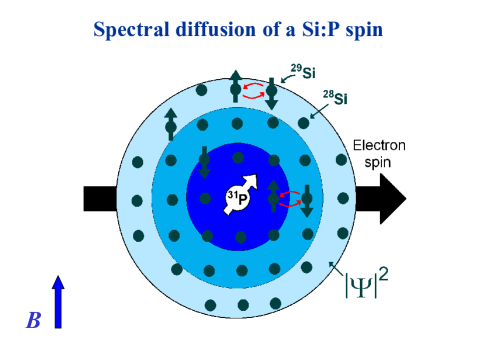
Figure 1: (Color online) The electron of a P donor in Si experiences spectral diffusion due to the spin dynamics of the enveloped bath of Si nuclei. Of the naturally occurring isotopes of Si, only ²⁹Si has a net nuclear spin, which may contribute to spectral diffusion by flip-flopping with nearby ²⁹Si. Natural Si contains about $5\%$ ²⁹Si or less through isotopic purification. Isotopic purification or nuclear polarization will suppress spectral diffusion in Si.

The spin decoherence mechanism known as spectral diffusion (SD) has a long historyherzog56 ; feher59 ; mims60_61 ; klauder62 ; zhidomirov69 ; chiba72 , and has been extensively studied recentlytyryshkin ; abe ; petta05 ; Delft ; desousa03b ; witzelHahnShort ; yaoHahn ; witzelHahnLong ; witzelCPMG ; yaoCDD ; yaoCDDlong ; witzelCDD ; SaikinLinkedCluster in the context of spin qubit decoherence. Consider a localized electron in a solid. This is our central spin. The electron spin could decohere through a number of mechanisms. In particular, spin relaxation would occur via phonon or impurity scattering in the presence of spin-orbit coupling, but these relaxation processes are strongly suppressed in localized systems and can be arbitrarily reduced by lowering the temperature and applying a strong external magnetic field, creating a large electronic Zeeman splitting. In the dilute doping regime of interest in quantum computation, where the localized electron spins are spatially well separated, a direct magnetic dipolar interaction between the electrons themselves is not an important dephasing mechanism.desousa03a Therefore, the interaction between the electron spin and the nuclear spin bath is the important decoherence mechanism at low temperatures and for localized electron spins. Now we restrict ourselves to a situation in the presence of an external magnetic field (which is the situation of interest to us) and consider the spin decoherence channels for the localized electron spin interacting with the lattice nuclear spin bath. Since the gyromagnetic ratios (and, hence, the Zeeman energies) for the electron spin and the nuclear spins are typically a factor of 2000 different (the electron Zeeman energy being larger), hyperfine-induced direct spin-flip transitions between electron and nuclear spins would be impossible (except as virtual transitions as will be discussed in Sec. II.1) at low temperature since phonons would be required for energy conservation. This leaves the indirect SD mechanism as the most effective electron spin decoherence mechanism at low temperatures and finite magnetic fields. The SD process is associated with the dephasing of the electron spin resonance due to the temporally fluctuating nuclear magnetic field at the localized electron site. These temporal fluctuations cause the electron spin resonance frequency to diffuse in the frequency space, hence the name spectral diffusion. These fluctuations result from the dynamics of the nuclear spin bath due to dipolar interactions with each other along with their hyperfine interactions with the qubit. This scenario is illustrated in Fig. 1. Nuclear spins in the spin bath flip-flop due to their mutual dipolar coupling (since the typical experimental temperature scale $\sim 100~{}\mbox{mK}$ is essentially an infinite temperature scale for the nuclear spins with nano-Kelvin scale coupling), and this leads to a temporally random magnetic-field fluctuation on the central spin, i.e., the electron.

II.1 Interactions

In the most general form, the SD Hamiltonian for the central spin decoherence problem may be written (in $\hbar=1$ unit)

$$\hat{\cal H} = \Omega_{e}\hat{S}_{z}+\sum_{n}\hat{\vec{I}}_{n}\cdot\bm{A}_{n}\cdot\hat{\vec{S}}$$

$${}+\sum_{n}\omega_{n}\hat{I}_{nz}+\sum_{n<m}\hat{\vec{I}}_{n}\cdot\bm{B}_{nm}\cdot\hat{\vec{I}}_{m},$$

where $\hat{\vec{S}}$ and $\hat{\vec{I}}_{n}$ are vectors of spin operators for the electron (central spin) and nucleus $n$ respectively, $\Omega_{e}$ and $\omega_{n}$ are their respective Zeeman energies (with an external magnetic field applied in the $z$ direction), and $\bm{A}_{n}$ and $\bm{B}_{nm}$ are tensors describing electronuclear and internuclear interactions respectively. Isotropic Fermi-contact hyperfine (HF) interactions typically dominate $\bm{A}_{n}$ (i.e., $\bm{A}_{n}=A_{n}\mathbbm{1}$) although anisotropic HF interactions, due to dipolar contributions, may also be important. Internuclear dipolar interactions often dominate $\bm{B}_{nm}$, though other local interactions between nuclei such as indirect exchange interactionsshulman55 ; shulman58 ; sundfors69 may also be significant.yaoHahn Typical energy scales are shown in Table 1 for convenience.

Table 1: Interactions and estimated energy scales. (A similar table appears in Ref. yaoCDDlong, .)

Interaction	Symbol	Scale ($\hbar=1$)	Scale ($k_{B}=1$)
Zeeman (electron)	$\Omega_{e}$	$10^{11}~{}\mbox{s}^{-1}$ a	$1~{}\mbox{K}$ a
Zeeman (nucleus)	$\omega_{n}$	$10^{8}~{}\mbox{s}^{-1}$ a	$1~{}\mbox{mK}$ a
Contact HF	$A_{n}$	$10^{6}~{}\mbox{s}^{-1}$ b	$10~{}\mbox{$\mu$K}$ b
Cumulative HF	${\cal A}=\sum_{n}A_{n}$	$\lesssim 10^{11}~{}\mbox{s}^{-1}$ c	$\lesssim 1~{}\mbox{K}$ c
Dipolar	$B_{nm}$	$10^{2}~{}\mbox{s}^{-1}$	$1~{}\mbox{nK}$
Indirect exchange	$B_{nm}^{\mbox{\scriptsize Ex}}$	$10^{2}~{}\mbox{s}^{-1}$	$1~{}\mbox{nK}$
HF mediated	$A_{nm}$	$10~{}\mbox{s}^{-1}$	$10^{-1}~{}\mbox{nK}$

^a With a magnetic field of about $1~{}\mbox{T}$.

^b In III-V compound quantum dots with $N\sim 10^{5}$ nuclei and also in Si:P donors.

^c In III-V compound quantum dots, ${\cal A}\sim 10^{11}~{}\mbox{s}^{-1}$. In Si:P donors, ${\cal A}\sim f\times 10^{10}~{}\mbox{s}^{-1}$, where $f$ is the fraction of ²⁹Si.

The HF energies are typically many orders of magnitude larger than internuclear dipolar energies: $\|\bm{A}_{n}\|\gg\|\bm{B}_{nm}\|$. By ignoring the $\bm{B}_{nm}$ term for a moment, decoherence may occur as a result of real or virtual electronuclear flip-flops via the HF interaction.Basel ; deng Such a process may be suppressed, however, by increasing the applied magnetic field due to a conservation of Zeeman energies. These Zeeman energies are given by $\Omega_{e}=\gamma_{S}B$ and $\omega_{n}=-\gamma_{n}B$, where $B$ is the applied magnetic-field strength, and $\gamma_{S}$ and $\gamma_{n}$ are gyromagnetic ratios of the electron and nucleus $n$, respectively (with $\gamma_{n}$ defined in an opposite sense as $\gamma_{S}$). Typically, $\gamma_{S}\sim 10^{3}\gamma_{n}$ so that the nuclear Zeeman energy is negligible relative to the electron’s Zeeman energy and the electron must overcome its Zeeman energy barrier in order to flip. In the limit of $\Omega_{e}\gg{\cal A}$, with ${\cal A}=\sum_{n}A_{n}$, HF-induced electronuclear flip-flops are effectively suppressed. When we reintroduce $\bm{B}_{nm}$, however, decoherence still occurs and is well defined in the $\Omega_{e}\rightarrow\infty$ limit because the electron spin will dephase as a result of nuclear field fluctuations induced by inter-nuclear interactions. This decoherence is spectral diffusion.

In the limit of a large applied field (formally we will say $\Omega_{e}\rightarrow\infty$), electron flips are completely suppressed. In this limit, the effective Hamiltonian becomes $\hat{\cal H}\approx\sum_{n}\omega_{n}\hat{I}_{nz}+\sum_{n}\left(\vec{A}_{n}\cdot\hat{\vec{I}}_{n}\right)\hat{S}_{z}+\sum_{n<m}\hat{\vec{I}}_{n}\cdot\bm{B}_{nm}\cdot\hat{\vec{I}}_{m}$, where $\vec{A}_{n}$ is the $z$ column vector of $\bm{A}_{n}$. We are free to drop $\Omega_{e}\hat{S}_{z}$ for any dynamical considerations now because it is a conserved energy in this limit. Effects due to anisotropic HF interactions may be treated independently of SD with a trivial disregard to internuclear interactions.witzelAHF For our purposes, therefore, we will treat only the $z$ component of $\vec{A}_{n}$ from the Fermi-contact HF interaction, which leaves us with

$$\hat{\cal H} \approx \sum_{n}A_{n}\hat{I}_{nz}\hat{S}_{z}+\sum_{n}\omega_{n}\hat{I}_{nz}+\sum_{n<m}\hat{\vec{I}}_{n}\cdot\bm{B}_{nm}\cdot\hat{\vec{I}}_{m},~{}~{}~{}$$ (2)

$$A_{n} = \frac{8\pi}{3}\gamma_{S}\gamma_{n}\hbar|\Psi(\bm{R}_{n})|^{2}.$$ (3)

Equation (3) gives Fermi-contact HF coupling constants that are proportional to the probability of the electron being at the nuclear site (the square of its wavefunction).

How large of a magnetic field must we apply for Eq. (2) to be a valid effective Hamiltonian? To be explicit, one may use quasidegenerate perturbation theory Winkler to systematically transform Eq. (II.1) into the block form $\hat{\cal H}\approx\sum_{\pm}\lvert\pm\rangle\hat{\cal H}_{\pm}\langle\pm\rvert$, where $\left\{\lvert+\rangle,\lvert-\rangle\right\}$ are the electron spin states. This transformation will be convergent if $\Omega_{e}\gg{\cal A}$, where ${\cal A}=\sum_{n}A_{n}$ is the maximum cumulative HF field. In III-V compound quantum dots, $\Omega_{e}\sim{\cal A}$ with an applied field of $1~{}\mbox{T}$, calling this approach into question; however, the $\Omega_{e}\gg{\cal A}$ condition is overly strict because this maximum HF field is never reached in a bath that is not fully polarized. It is more relevant to consider how higher orders of this transformation [Eq. (2) represents the zeroth order] compare with the internuclear $\bm{B}_{nm}$ coupling term to generate decoherence. In the next order of the transformation, HF-mediated interactions between nonlocal nuclei emerge. This interaction, wellknownslichter ; bloembergen55 as the Ruderman-Kittel-Kasenya-Yosida interaction, results from virtual electron spin flips and is suppressed with a large applied magnetic field. This next order contribution to the Hamiltonian is given byyaoHahn

$$\hat{\cal H}^{\mbox{\scriptsize HFM}}=\sum_{n\neq m}A_{nm}\hat{I}_{n+}\hat{I}_{m-}\hat{S}_{z},$$ (4)

where $A_{nm}=A_{n}A_{m}/\Omega_{e}$. In applying this transformation, we must slightly rotate the basis states; this results in a “visibility” lossshenvi05 of coherence estimated asyaoHahn $\sum_{n}\left(A_{n}/\Omega_{e}\right)^{2}$ and is certainly small for a large bath in which $\Omega_{e}\gtrsim{\cal A}$. In this paper, we will restrict ourselves to the $\Omega_{e}\rightarrow\infty$ limit and merely mention how HF-mediated or other higher order interactions may play a role.

Direct interactions between nuclei are often dominated by their magnetic dipoles with the form

$$\hat{\cal H}^{\mbox{\scriptsize D}}_{nm}=\frac{\gamma_{n}\gamma_{m}\hbar}{2}\left[\frac{\hat{I}_{n}\cdot\hat{I}_{m}}{R_{nm}^{3}}-\frac{3(\hat{I}_{n}\cdot{\bm{R}_{nm}})(\hat{I}_{m}\cdot{\bm{R}_{nm}})}{R_{nm}^{5}}\right].$$ (5)

The dipolar interaction between nuclear spins in semiconductors has a typical strength of $\hat{\cal H}^{\mbox{\scriptsize D}}_{nm}\sim 10^{2}~{}s^{-1}$, which is much smaller than typical nuclear Zeeman energies of about $10^{8}~{}s^{-1}$ in an applied field of $1~{}T$. Therefore, energy conservation arguments allow us to neglect any term that changes the total Zeeman energy of the nuclei. This leaves the following Zeeman energy-conserving secularabragam62 ; slichter part of the interaction:

$$\sum_{n<m}\hat{\cal H}^{\mbox{\scriptsize D}}_{nm} \approx \frac{1}{2}\sum_{n\neq m}B_{nm}\left[\delta_{\gamma_{n},\gamma_{m}}\hat{I}_{n+}\hat{I}_{m-}-2\hat{I}_{nz}\hat{I}_{mz}\right],~{}~{}~{}$$ (6)

$$B_{nm} = -\frac{1}{2}\gamma_{n}\gamma_{m}\hbar\frac{1-3\cos^{2}{\theta_{nm}}}{R^{3}_{nm}},$$ (7)

where $R_{nm}$ is the length of the vector joining nucleus $n$ and nucleus $m$, and $\theta_{nm}$ is the angle of this vector relative to the $z$ magnetic-field direction. The $\delta_{\gamma_{n},\gamma_{m}}$ denotes that the flip-flop interaction between nuclei with different gyromagnetic ratios should be excluded because of Zeeman energy conservation in the same way that the nonsecular part of the dipolar interaction is suppressed. This occurs, for example, in GaAs because the two isotopes of Ga and the isotope of As that are present have significantly different gyromagnetic ratios. This secular interaction corresponds to a $\bm{B}_{nm}$ matrix for Eq. (2), with $B_{nm}$, $B_{nm}$, and $-2B_{nm}$ along the diagonal, respectively, in the $x$-$y$-$z$ spin basis for a pair of nuclei having the same gyromagnetic ratios. (The $\hat{I}_{nz}\hat{I}_{mz}$ term plays an insignificant role, which is why we use the same $B_{nm}$ symbol, in different fonts, for the scalar and tensor).

In addition to the dipolar interactions between nuclei, an indirect nuclear-spin exchange,bloembergen55 ; anderson55 ; shulman55 ; shulman58 ; sundfors69 which is mediated by virtual electron-hole pairs, may also have a significant quantitative impact on SD in III-V materials.yaoHahn This interaction takes the form

$$\hat{\cal H}^{\mbox{\scriptsize Ex}}_{nm}=B^{\mbox{\scriptsize Ex}}_{nm}\hat{I}_{n}\cdot\hat{I}_{m}.$$ (8)

The corresponding $\bm{B}_{nm}$ is $\bm{B}_{nm}^{\mbox{\scriptsize Ex}}=B^{\mbox{\scriptsize Ex}}_{nm}\mathbbm{1}$. The leading contribution to this pseudoexchange interaction for nearest neighbors may be expressed as anderson55 ; shulman55

$$B_{nm}^{\mbox{\scriptsize Ex}}=\frac{\mu_{0}}{4\pi}\frac{\gamma_{n}^{\mbox{\scriptsize Ex}}\gamma_{m}^{\mbox{\scriptsize Ex}}}{{\bm{R}}_{nm}^{3}}\frac{a_{0}}{{\bm{R}}_{nm}},$$ (9)

where $\gamma^{\mbox{\scriptsize Ex}}_{n}$ is the effective gyromagnetic ratio determined by a renormalization of the electron charge density.yaoHahn This interaction has been experimentally studied many years ago.shulman55 ; shulman58 ; sundfors69 In GaAs quantum dots, these interactions can be comparable to the direct dipolar interactions. There may be other local interactions between nuclei in the bath, such as the indirect pseudodipolar interaction bloembergen55 or internuclear quadrapole interaction, but the dipolar and indirect exchange interactions alone account for nuclear magnetic resonance line shapes.yaoHahn ; shulman55 ; shulman58 ; sundfors69 In any case, all such local interactions may easily be included in our formalism.

To summarize and put everything in a convenient general form, we approximate our Hamiltonian as $\hat{\cal H}\approx\sum_{\pm}\lvert\pm\rangle\hat{\cal H}_{\pm}\langle\pm\rvert$ where

$$\hat{\cal H}_{\pm} = \pm\hat{\cal H}_{eb}+\epsilon\hat{\cal H}_{bb}.$$ (10)

$\hat{\cal H}_{eb}$ is the electron dependent part that plays the role of coupling the electron spin to the bath, and $\hat{\cal H}_{bb}$ includes secular (preserving nuclear Zeeman energy) bath-bath, i.e., internuclear, interactions such as the secular dipolar interaction [Eq. (6)] and the exchange interaction [Eq. (8)]. Zeeman energies are omitted from this Hamiltonian because they are preserved by all included interactions and, thus, not relevant to the dynamics.

In the $\Omega_{e}\rightarrow\infty$ limit,

$$\hat{\cal H}_{eb}\approx\frac{1}{2}\sum_{n}A_{n}\hat{I}_{nz},$$ (11)

with a factor of $1/2$ from the magnitude of the electron spin, and $A_{n}$ given by Eq. (3) with a proportionality to the square of the electron wavefunction at site $n$. To validate this approximate form, one may consider the effects of higher order interactions of the canonical transformation, such as the HF-mediated interactions [Eq. (4)] that contribute to $\hat{\cal H}_{eb}$ (due to its $\hat{S}_{z}$ dependence). These higher order interactions introduce additional decoherence mechanisms that will shorten coherence times at lower magnetic fields. The main consideration of this paper is the decoherence that may not be removed by simply increasing the magnetic-field strength and is applicable in the limit of a large applied field at the point where decoherence is insensitive to the strength of the applied field.

II.2 Decoherence

We characterize decoherence as the expectation value of the electron spin over the evolution of the experiment. Since we consider a dephasing-only Hamiltonian of the form $\hat{\cal H}\approx\sum_{\pm}\lvert\pm\rangle\hat{\cal H}_{\pm}\langle\pm\rvert$, we need only deal with dephasing decoherence. Dephasing decoherence involves only the transverse component of the electron spin. For a given experiment, we define the up and down evolution operators, $\hat{U}^{\pm}$, as evolution operators for the bath given an initially up or down electron spin. If we just have free evolution for a time $t$, then $\hat{U}_{\pm}=\hat{U}^{\pm}_{0}=\exp{\left(-i\hat{\cal H}_{\pm}t\right)}$. In general, we can consider an experiment with a sequence of $\pi$ pulses that flip the electron spin between periods of free evolution time $\tau_{j}$, so that

$$\hat{U}_{\pm}=...\exp{\left(-i\hat{\cal H}_{\mp}\tau_{2}\right)}\exp{\left(-i\hat{\cal H}_{\pm}\tau_{1}\right)}.$$ (12)

The transverse component of the expectation value of the electron spin will then decay, in magnitude, by a factor of $\left\|\left\langle\hat{U}_{-}^{{\dagger}}\hat{U}_{+}\right\rangle\right\|=\left\|\langle\hat{W}\rangle\right\|$, where $\hat{W}\equiv\hat{U}_{-}^{{\dagger}}\hat{U}_{+}$, $\langle...\rangle$ denotes an appropriately weighted average over the bath states, and $\|...\|$ takes the magnitude of the resulting complex number. The coherence decay is thus characterized by $\left\|\langle\hat{W}\rangle\right\|$. In an echo experiment, one initializes an ensemble of pure electron spin state in some transverse direction, applies a sequence of $\pi$ pulses designed to refocus the spins, and observes an echo signal, $v_{E}=\left\|\langle\hat{W}\rangle\right\|$, at the end of the experiment.

Given an arbitrary initial bath density matrix written in the form $\hat{\rho}_{b}\equiv\sum_{j}P_{j}\lvert{\cal B}_{j}\rangle\langle{\cal B}_{j}\rvert$, we may average $\hat{W}$ over bath states with

$$\langle\hat{W}\rangle=\sum_{j}P_{j}\langle{\cal B}_{j}|\hat{W}|{\cal B}_{j}\rangle,$$ (13)

where each $\lvert{\cal B}_{j}\rangle$ is a different bath state. By referring to the energy scale estimates of Table 1, temperatures on the $\mbox{mK}-\mbox{K}$ scale are justifiably treated as infinite with respect to the nK scale intrabath interactions. The remaining Zeeman and Fermi-contact HF interactions in our approximate Hamiltonian quantize the nuclear spins in the $z$ direction (involving only $\hat{I}_{nz}$ nuclear spin operators) and, thus, we can approximate the initial bath density matrix as a mixed state composed of uncorrelated pure nuclear spin states in this basis so that

$$\lvert{\cal B}_{j}\rangle\approx\prod_{\otimes~{}n}\left(\sum_{m}p_{nm}\lvert I_{n},m\rangle_{n}\right),$$ (14)

where $I_{n}$ is the magnitude of the $n$th nuclear spin and $\lvert I_{n},m\rangle_{n}$ represents the state of the $n$th nuclear spin with a $z$ projection of $m$. The cluster approximation in Sec. III.1 will make use of the assumption that the bath is initially uncorrelated (at least, approximately). Section IV will use the $z$ quantization as a further convenience.

II.3 Dynamical decoupling pulse sequences

If we simply let the system freely evolve, the decay of the electron spin expectation value strongly depends on the type of averaging we perform over bath states. If we consider an ensemble of electron spins, each with its own bath, then we will see rapid electron spin dephasing simply due to the distribution of HF nuclear fields, $\sum_{n}A_{n}\hat{I}_{nz}/2$. This is known as inhomogeneous broadening because it broadens the electron spin precessional frequency due to inhomogeneity of the effective magnetic field. This, however, is an artifact of the ensemble or our lack of knowledge of the effective nuclear field of a static bath and not true decoherence. If we consider a single electron spin with a known nuclear field, or a homogeneous ensemble which may be obtained through mode locking,modeLock for example, we arrive at a dynamical decoherence known as FID. In our dephasing model, FID can only arise from interactions among bath elements, such as local dipolar or nonlocal HF-mediated interactions.

Traditionally,herzog56 nonhomogeneously broadened coherence is measured from Hahn spin echoes. The Hahn echo sequence simply involves a single $\pi$ rotation midway through the evolution such that $\hat{U}_{\pm}(t)=\hat{U}^{\pm}_{1}(t)=\hat{U}^{\mp}_{0}(\tau)\hat{U}^{\pm}_{0}(\tau)$, with $\tau=t/2$. We denote this sequence with $\tau\rightarrow\pi\rightarrow\tau$: free evolution for a time $\tau$, then a $\pi$ pulse, then free evolution for a time $\tau$ again, with the arrows indicating the sequence ordered in time. This sequence will reverse the effect of any inhomogeneous static field. What remains is SD induced by a dynamical nuclear bath. It is important to note, however, that the effects of the Hahn echo go beyond the elimination of inhomogeneous broadening. The Hahn echo is also a DD sequence,longKhodjasteh in which the first order of the Magnus expansionMagnus is removed by the fact that the time-averaged Hamiltonian, proportional to $\hat{\cal H}_{+}+\hat{\cal H}_{-}\propto\hat{\cal H}_{b}$, decouples the qubit from the bath. For this reason, the Hahn echo does not have the same effect as homogeneous (or single qubit) free induction decay.yaoHahn In particular, the Hahn echo removes the lowest-order effects of HF-mediated interactions.yaoHahn This is because HF-mediated interactions, having an $\hat{S}_{z}$ factor [Eq. (4)], belong to $\hat{\cal H}_{eb}$, and if we consider only HF-mediated intrabath interactions, then $\hat{U}_{1}^{\pm}=\exp{\left(\pm i\hat{\cal H}_{eb}\tau\right)}\exp{\left(\mp i\hat{\cal H}_{eb}\tau\right)}=\hat{\mathbbm{1}}$.

Given a DD sequence, such as the Hahn echo for a dephasing system, coherence over a given net amount of time may be increased through a rapid repetition of the basic sequence. This strategy, known as bang-bang in the quantum information community,ViolaPRL05 gives coherence enhancement at the cost of more frequent applications of $\pi$ pulses. Pulses must be applied more frequently because errors due to higher order terms of the Magnus expansion pile up over the course of the sequence. A better strategy is to use recursion, rather than repetition, to generate concatenated sequences.KhodjastehPRL Such CDD, with the Hahn echo as the base sequence, has been shownwitzelCDD to be effective for the SD problem. In fact, with each concatenation, we demonstrated, in Ref. witzelCDD, , coherence enhancement with an increase in the time between pulses (let alone, the net sequence time).

With $l>0$ levels of concatenation, our CDD pulse sequence is recursively defined by KhodjastehPRL $\mbox{p}_{l}:=\mbox{p}_{l-1}\rightarrow\pi\rightarrow\mbox{p}_{l-1}\rightarrow\pi$, with $\mbox{p}_{0}:=\tau$. CDD with $l=0$ is simply free evolution. At $l=1$, we have $\mbox{p}_{1}:=\tau\rightarrow\pi\rightarrow\tau\rightarrow\pi$, which is simply the Hahn echo (with an extra $\pi$ pulse at the end to bring the electron spin back to its original phase apart from the decoherence). With each concatenation, we do to the previous sequence what the Hahn echo does to free evolution and, in this way, we obtain improved DD. This sequence may be simplified by noting that two $\pi$ pulses in sequence do nothing. Thus,

$$\mbox{p}_{l}:=\left\{\begin{array}[]{ll}\mbox{p}_{l-1}\rightarrow\pi\rightarrow\mbox{p}_{l-1}&,~{}\mbox{odd}~{}l\\ \mbox{p}_{l-1}\rightarrow\mbox{p}_{l-1}&,~{}\mbox{even}~{}l\end{array}\right.$$ (15)

(again, arrows indicate sequences ordered in time) and the up and down evolution operators at level $l$ have the recursive form ofyaoCDD

$$\hat{U}_{l}^{\pm}=\hat{U}_{l-1}^{\mp}\hat{U}_{l-1}^{\pm}.$$ (16)

Recently, a series of DD sequences was discovered by UhrigUhrigSequence to be optimal in the number of pulses for the spin-boson model. The $n$-pulse sequence in this series may be defined by

$$\tau_{j}=\frac{1}{2}\left[\cos{\left(\frac{\pi(j-1)}{n+1}\right)}-\cos{\left(\frac{\pi j}{n+1}\right)}\right]$$ (17)

for $1\leq j\leq n+1$. Unlike CDD, Uhrig DD (UDD) requires only a linear (rather than exponential) overhead in the number of pulses for each order of coherence enhancement. Furthermore, UDD was shownUDD to kill off successive orders in a time expansion in a completely model-independent manner. The UDD sequence has a strong advantage over CDD in its linear versus exponential scaling of the number of pulses; however, it is effective only when a time expansion is convergent, while CDD is also effective in the intrabath perturbation for SD (this is important since $B_{nm}\ll A_{n}$).

In Sec. IV, we will discuss the wavefunction dependence in the short-time approximation. It would be natural to discuss this in the context of the UDD series since UDD is effective in this short-time limit. However, the methods of Sec. IV.3 work for the CDD series but, unfortunately, do not work for the UDD series. In this work, we therefore focus attention on FID and the CDD series. Note, however, that the UDD and CDD series are the same for levels zero (FID), 1 (Hahnherzog56 ), and 2 (CPMGMeiboom ; witzelCPMG ).

III Cluster method

In this section, we review our cluster expansion methodwitzelHahnShort ; witzelHahnLong for solving the SD problem in a particularly simple and illuminating form. Section III.1 gives the basic cluster expansion result, the cluster approximation, in which we equate $\langle\hat{W}\rangle$ [see Sec. II.2] to the exponentiation of single-cluster contributions. This is useful because perturbation theory cannot be directly applied to $\langle\hat{W}\rangle$, but it can be applied to its single-cluster contributions (it is the multicluster contributions that are particularly problematic for perturbation theories due to the large number of possibilities in combing different clusters). We consider aspects of such perturbation expansions in Sec. III.2 that will be relevant to Sec. IV.

III.1 Cluster approximation

The cluster expansion is based on the fact that our $\hat{\cal H}_{\pm}$ Hamiltonians couple nuclei via relatively weak pairwise interactions in a large bath with $N$ nuclei (any $n$-way interactions could justify such an approximation as long as $n\ll N$). The $\hat{W}$ operator, which is the product of evolution operators arising from $\hat{\cal H}_{\pm}$, can, in principle, be expanded into a sum of products of the Hamiltonian interaction elements. The interaction elements of each such term will uniquely determine a set of clusters of nuclei; each cluster, with respect to this term, may involve interactions among itself but not among any other cluster, and no cluster may be divided into further subclusters. For example, a term with $B_{1,2}I_{1+}I_{2-}B_{3,4}I_{3+}I_{4-}$ forms two clusters, $\{1,2\}$ and $\{3,4\}$, while $B_{1,2}I_{1+}I_{2-}B_{2,3}I_{2+}I_{3-}$ forms a single cluster of $\{1,2,3\}$. The term “cluster” implies proximity among the member nuclei as applicable to local dipolar interactions; however, we may also treat nonlocal HF-mediated interactions using the term cluster in a more general sense as a set of nuclei that are interconnected by interactions under consideration.

If one considers a perturbative expansion of $\langle\hat{W}\rangle$ with respect to the pairwise interactions, one immediately faces the problem that the number of terms of $\hat{W}$ scales in powers of $N$ with successive inclusion of the pairwise interactions, destroying any hope of convergence when $N$ is large. To resolve this problem, let us first partition $\hat{W}$ according to the number of clusters involved in each term such that

$$\hat{W}=\sum_{p=0}^{N}\hat{W}^{[p]},$$ (18)

where we define $\hat{W}^{[p]}$ as the sum of the terms from $\hat{W}$ that involve $p$ independent clusters. Note that $\hat{W}^{[0]}=\hat{\mathbbm{1}}$. By considering only local interactions (e.g., dipolar), then it is apparent that a perturbative expansion of $\langle\hat{W}^{[1]}\rangle$ with respect to the pairwise interactions does not suffer from the adverse $N$ scaling suffered by $\langle\hat{W}\rangle$ because, when interactions are local, there are ${\cal O}\left(N\right)$ clusters of any size. Even with nonlocal interactions, the perturbative expansion of $\langle\hat{W}^{[1]}\rangle$ is a generally significantly better controlled expansion for large $N$ than that of $\langle\hat{W}\rangle$.

Assume that, arising from a perturbative expansion with respect to the pairwise interactions, $\hat{W}^{[1]}$ is well approximated when only including contributions due to clusters of some maximum size that is much less than $N$. Along with our assumption that the bath nuclei are initially uncorrelated, Appendix A shows that $\langle\hat{W}^{[k]}\rangle\approx\langle\hat{W}^{[1]}\rangle^{k}/k!$ [Eq. (59)]. This approximation breaks down as $k$ becomes significant relative to $N$; however, for a large enough bath where the previous assumptions are met,

$$\langle\hat{W}\rangle\approx\exp{\left(\langle\hat{W}^{[1]}\rangle\right)}$$ (19)

and

$$v_{E}=\left\|\langle\hat{W}\rangle\right\|\approx\exp{\left(\operatorname{Re}{\left\{\langle\hat{W}^{[1]}\rangle\right\}}\right)}.$$ (20)

A formalized cluster expansion, with a discussion on convergence tests, is presented in Ref. witzelHahnLong, . The cluster approximation presented in this subsection gives an equivalent result with a simpler derivation.

III.2 Single-cluster perturbation

Given the result of Eq. (20), we have reduced the problem of SD decoherence to that of perturbatively treating $\operatorname{Re}{\left\{\langle\hat{W}^{[1]}\rangle\}\right\}}$. That is, we wish to consider a perturbative expansion of $\hat{W}$ where we neglect terms involving multiple clusters. To be consistent with the cluster approximation, such a perturbation should be directly or indirectly tied to cluster size so that large clusters may be neglected. To this effect, we may perturbatively treat the pairwise interactions (the intrabath perturbation) or we may consider a time expansion which, in a sense, perturbatively treats all of the interactions (e.g., HF, dipolar, and HF mediated); in either case, larger clusters require more interaction factors and thereby increase the order of the perturbation.

In this section, we will consider general perturbative properties that apply to both the intrabath and time perturbation expansions. In Sec. IV, we will specifically consider the time perturbation and see how it may be used in the formulation of a convenient continuum approximation. In a perturbation whose order increases with increasing cluster size, the lowest order of $\langle\hat{W}\rangle-1$ is equivalent to the same order of $\langle\hat{W}^{[1]}\rangle$ because terms of $\hat{W}$ with multiple clusters are automatically higher order terms (products of lower order terms). To the lowest order, then, and in the context of CDD with $l$ levels of concatenation, we will consider $\langle\hat{W}\rangle$.

By noting that $\hat{U}^{\pm}_{l}$ are unitary operators such that $\left[\hat{U}^{\pm}_{l}\right]^{{\dagger}}\hat{U}^{\pm}_{l}=\hat{\mathbbm{1}}$, we may write

$$\operatorname{Re}{\left\{\left\langle\hat{W}_{l}\right\rangle\right\}} = \frac{1}{2}\left\langle\left[\hat{U}^{-}_{l}\right]^{{\dagger}}\hat{U}_{l}^{+}+\left[\hat{U}_{l}^{+}\right]^{{\dagger}}\hat{U}_{l}^{-}\right\rangle$$ (21a)

$$= 1-\frac{1}{2}\left\langle\Delta_{l}^{{\dagger}}\Delta_{l}\right\rangle,$$ (21b)

where we define $\Delta_{l}\equiv\hat{U}^{+}_{l}-\hat{U}^{-}_{l}$. Thus, $\left\langle\Delta_{l}^{{\dagger}}\Delta_{l}\right\rangle$ gives a measure of the decoherence. By applying the recursive definitions for the $\hat{U}^{\pm}_{l}$ evolution operators [Eq. (16)],

$$\hat{\Delta}_{l}\equiv\hat{U}_{l}^{+}-\hat{U}_{l}^{-}=\left[\hat{U}_{l-1}^{-},\hat{U}_{l-1}^{+}\right]=\left[\hat{U}_{l-1}^{-},\hat{\Delta}_{l-1}\right],$$ (22)

since $\hat{U}^{-}_{l-1}$ commutes with itself.

Let us consider a perturbation with a smallness parameter $\lambda$ in which $\hat{U}_{l}^{\pm}=\hat{\mathbbm{1}}+{\cal O}\left(\lambda\right)$ for all $l\geq l_{0}$ for some $l_{0}$. Two such perturbations are the time expansion with $\lambda=\tau$, $l_{0}=0$ (since no evolution occurs in the $\tau\rightarrow 0$ limit) and intrabath perturbation with $\lambda=\epsilon$, $l_{0}=1$ (since there is a perfect spin echo refocusing in the $\epsilon\rightarrow 0$ limit). Because the identity commutes with anything, it is easy to see from Eq. (22) that $\hat{\Delta}_{l}={\cal O}\left(\lambda\right)\times\hat{\Delta}_{l-1}$ for all $l>l_{0}$; this proves that we get successive cancellations of the low-order perturbation ($\tau$ or $\epsilon$) with each concatenation of the sequence.witzelCDD The lowest order result is given by

$$\hat{\Delta}_{l}\approx\lambda\left[\left.\frac{d}{d\lambda}\hat{U}_{l-1}^{-}\right\rvert_{\lambda=0},\hat{\Delta}_{l-1}\right],~{}\forall~{}l>l_{0}.$$ (23)

Conveniently, for all $l>l_{0}$,

$$\left.\frac{d}{d\lambda}\hat{U}_{l}^{\pm}\right\rvert_{\lambda=0} = \left.\frac{d}{d\lambda}\hat{U}_{l-1}^{+}\right\rvert_{\lambda=0}+\left.\frac{d}{d\lambda}\hat{U}_{l-1}^{-}\right\rvert_{\lambda=0}$$

$$= 2^{l-l_{0}}\left.\frac{d}{d\lambda}\left(\hat{U}_{l_{0}}^{+}+\hat{U}_{l_{0}}^{-}\right)/2\right\rvert_{\lambda=0},$$

so that Eq. (23) becomes

$$\hat{\Delta}_{l}\approx\lambda\left\{\begin{array}[]{ll}2^{l-l_{0}-1}\left[\left.\frac{d}{d\lambda}\left(\frac{\hat{U}_{l_{0}}^{+}+\hat{U}_{l_{0}}^{-}}{2}\right)\right\rvert_{\lambda=0},\hat{\Delta}_{l-1}\right]&,~{}l>l_{0}\\ \left.\frac{d}{d\lambda}\left(\hat{U}_{l_{0}}^{+}-\hat{U}_{l_{0}}^{-}\right)\right\rvert_{\lambda=0}&,~{}l=l_{0}\end{array}\right..$$ (25)

Note that in the $l=l_{0}+1$ case, Eq. (22) yields

$$\hat{\Delta}_{l_{0}+1}\approx\lambda^{2}\left.\left[\frac{d}{d\lambda}\hat{U}_{l_{0}}^{-},\frac{d}{d\lambda}\hat{U}_{l_{0}}^{+}\right]\right\rvert_{\lambda=0},$$ (26)

which is equivalent to the corresponding case in Eq. (25) recalling that any operator commutes with itself.

IV Wavefunction dependence in the short time limit

In this section, we use the formalism developed in Sec. III, with the cluster approximation and general perturbation formulation of Sec. III.2, to derive results applicable in a short-time limit and use these results to formulate a continuum approximation useful for understanding the dependence of spectral diffusion on the shape of the electron wavefunction. In Sec. IV.1, we apply the general results of Sec. III.2 to obtain the lowest time perturbation results of $\operatorname{Re}{\{\langle\hat{W}^{[1]}\rangle\}}$. This is done for the cases of free induction decay and concatenated echoes. Section IV.2 shows how the nuclear dependent and electron dependent parts of this lowest-order time perturbation solution may be separated in a way that allows us to generically treat the bath for any electron wavefunction. Section IV.3 takes this one step further by treating the bath as a continuum so that we may obtain results via integration for any given electron wavefunction. In Sec. IV.4, we discuss the circumstances in which the time expansion may or may not be applicable.

IV.1 Time perturbation

Section III.2 considered the perturbations of concatenated Hahn sequences in a general sense in the context of the cluster approximation of Sec. III.1. Now we are specifically interested in the time expansion. We first address this in the case of FID and then treat the Hahn sequence and its concatenations.

IV.1.1 Free induction decay

The $l=0$ result of $\hat{\Delta}=\hat{U}_{+}-\hat{U}_{-}$, without any pulses, gives $\Delta_{0}=-2i\hat{\cal H}_{eb}\tau$. Where $\hat{\cal H}_{eb}=\sum_{n}A_{n}\hat{I}_{nz}/2$, this result for $\Delta_{0}$ is simply due to inhomogeneous broadening. In the case of free induction decay, we are not concerned with inhomogeneous broadening and would like to obtain the SD decoherence of a single electron spin (or a mode-locked ensemblemodeLock ). We may do this by entering the rotating frame of reference for the electron precessing in the nuclear field. This may be done, effectively, by making the transformations, $\hat{U}_{0}^{\pm}(t)\rightarrow\hat{U}_{0}^{\pm}(t)\exp{\left(\pm i\hat{\cal H}_{eb}t\right)}$. for free induction decay, we then obtain

$$\hat{\Delta}_{0}=\left[\hat{\cal H}_{eb},\hat{\cal H}_{b}\right]t^{2}.$$ (27)

The free induction decay is then given by Eq. (20) via Eq. (21b) with this form of $\hat{\Delta}_{0}$.

IV.1.2 Concatenated dynamical decoupling

We now consider the Hahn echo sequence and its concatenations: $l\geq 1$. There is no need to go into a rotating frame as we did for FID because these sequences automatically reverse the effects of inhomogeneous broadening. We will apply Eq. (25) by using $\lambda=\tau$. In the limit of $\tau\rightarrow 0$, no evolution can occur, so it is apparent that $\left.\hat{U}_{0}^{\pm}\right\rvert_{\tau=0}=\hat{\mathbbm{1}}$ and, thus, $l_{0}=0$ in this context. For $l=1$, the Hahn echo [Eq. (25)] becomes

$$\hat{\Delta}_{1} \approx 2\left[\hat{\cal H}_{eb},\hat{\cal H}_{b}\right]\tau^{2}.~{}~{}~{}$$ (28)

Note that there is a simple relationship between Eqs. (28) and (27) for the Hahn echo and FID, respectively. The relationship is not so simple when we move away from the $\Omega_{e}\rightarrow\infty$ limit and consider HF-mediated interactions. In that situation, discussed in Ref. yaoHahn, , the lowest order contribution to FID in the time expansion will come from HF-mediated interactions but this lowest order effect will be cancelled in the Hahn echo.

To consider concatenations of the echo, we simply apply the recursion of Eq. (25) to obtain

$$\hat{\Delta}_{l} = -2^{(l^{2}-l+2)/2}\left[...\left[\left[\hat{\cal H}_{eb},\hat{\cal H}_{b}\right],\hat{\cal H}_{b}\right],...\right]\left(i\tau\right)^{l+1}$$ (29)

$${}+{\cal O}\left(\tau^{l+2}\right),~{}~{}\forall~{}l>0,$$

with $l$ nested commutations abbreviated by $...$’s. As a result of these nested commutations and as observed in Ref. witzelCDD, , each concatenation introduces larger cluster sizes to the lowest-order expression (i.e., each time we commute with $\hat{\cal H}_{b}$, we may introduce an additional nuclear site to any term of this operator).

IV.2 Pair “correlations”

A reasonable assumption for many solid-state spin baths is that the bath Hamiltonian $\hat{\cal H}_{b}$, which excludes qubit-bath interactions, is homogeneous. That is, sites that are equivalent in terms of the Bravais lattice are equivalent with regard to bath interactions. A notable exception to this is where isotopes in the lattice are interchangeable; for example, three different isotopes of Si may occupy any lattice site in Si, and two different isotopes of Ga may occupy the Ga sublattice in GaAs. However, if we simply want to know the decoherence that results from averaging different types of isotopic configurations, then we may regard the bath (apart from the qubit interactions) as homogeneous and use isotopic probabilities in expressions for $\hat{\cal H}_{b}$. Then the only inhomogeneity is in the interactions with the qubit, $\hat{\cal H}_{eb}$. We can then factor out this inhomogeneous part and compute the rest in a way that is independent of the qubit interactions. This will be convenient, for example, when analyzing a quantum dot in which the wavefunction of the electron (whose spin represents the qubit) can take on many shapes and sizes.

By referring to Eqs. (27) and (29), we can make the following factorization of the homogeneous and nonhomogeneous parts of $\left\langle\hat{\Delta}_{l}^{{\dagger}}\hat{\Delta}_{l}\right\rangle$ [determining SD via Eqs. (21b) and (20)]:

$$\frac{1}{2}\left.\left\langle\hat{\Delta}_{l}^{{\dagger}}\hat{\Delta}_{l}\right\rangle\right\rvert_{\Omega_{e}\rightarrow\infty} = \sum_{n,m}A_{n}^{*}A_{m}f_{n,m}^{(l)}\tau^{p}$$

$${}+{\cal O}\left(\tau^{p+2}\right),~{}~{}~{}~{}$$

where

$$p(l)=\left\{\begin{array}[]{ll}4&,~{}l=0\\ 2l+2&,~{}l>0\end{array}\right..$$ (31)

For $l=0$ (FID),

$$f_{n,m}^{(0)} = \frac{1}{2}\left\langle\left[\hat{F}_{nz}^{(0)}\right]^{{\dagger}}\hat{F}_{mz}^{(0)}\right\rangle,$$ (32)

$$\hat{F}_{nz}^{(0)} = \left[\hat{I}_{nz},{\hat{H}}_{b}\right],$$ (33)

and for $l>0$,

$$f_{n,m}^{(l)} \equiv (-)^{(l+1)}2^{(l^{2}-l+1)}\left\langle\left[\hat{F}_{nz}^{(l)}\right]^{{\dagger}}\hat{F}_{mz}^{(l)}\right\rangle,~{}~{}~{}~{}$$ (34)

$$\hat{F}_{nz}^{(l)} = \left[...\left[\left[\hat{I}_{nz},{\hat{H}}_{b}\right],{\hat{H}}_{b}\right],...\right].$$ (35)

where the $...$’s again denote $l$ nested commutations.

Since we assume the high field limit where secular coupling $\hat{\cal H}_{b}$ preserves nuclear polarization, $\left[\hat{\cal H}_{b},\sum_{n}\hat{I}_{nz}\right]=0$ so that $\sum_{m}f_{n,m}^{(l)}=\sum_{m}f_{m,n}^{(l)}=0$ for any $n$. Then, $f_{n,n}^{(l)}=-\sum_{m\neq n}\left(f_{n,m}^{(l)}+f_{m,n}^{(l)}\right)/2$. By using this fact, we may rewrite Eq. (IV.2) in terms of the differences of the HF constants; after all, if $A_{n}$ is the same for all nuclei, there is no nuclear induced spectral diffusion in the high field limit (nuclear flip-flops would have no effect on the electron). We will assume that the HF constants are real, $A_{n}=A_{n}^{*}$, as is the case for the Fermi-contact interaction [Eq. (3)]. Then,

$$\sum_{n,m}A_{n}A_{m}f_{n,m}^{(l)} = \frac{1}{2}\sum_{n\neq m}A_{n}A_{m}\left(f_{n,m}^{(l)}+f_{m,n}^{(l)}\right)$$

$${}+\sum_{n}A_{n}^{2}f_{n,n}^{(l)}$$

$$= -\frac{1}{4}\sum_{n\neq m}(A_{n}-A_{m})^{2}\left(f_{n,m}^{(l)}+f_{m,n}^{(l)}\right).$$

Thus, in the short-time limit of Eq. (IV.2),

$$\frac{1}{2}\left\langle\hat{\Delta}_{l}^{{\dagger}}\hat{\Delta}_{l}\right\rangle\approx-\frac{1}{2}\sum_{n\neq m}(A_{n}-A_{m})^{2}\operatorname{Re}{\left\{f_{n,m}^{(l)}\right\}}\tau^{p}.$$ (37)

The homogeneous part is represented by $f_{n,m}^{(l)}$, and by exploiting this homogeneity, we note that this function is equivalent when we shift by any Bravais lattice vector, $\vec{R}$: $f^{(l)}(\vec{r}_{n},\vec{r}_{m})\equiv f_{n,m}^{(l)}=f^{(l)}(\vec{r}_{n}-\vec{R},\vec{r}_{m}-\vec{R})$. We may then relate any $\vec{r}_{n}-\vec{R}$ to one of the basis sites of the Bravais lattice, so then, with $b$ representing the corresponding basis site of $\vec{r}_{n}$, we may write

$$f_{n,m}^{(l)}=f_{b}^{l}(\vec{r}_{n}-\vec{r}_{m}).$$ (38)

IV.3 Continuum approximation

The pair correlation formulation above is particularly convenient in the context of a continuum approximation for HF coupling constants. From the Fermi-contact HF interaction [Eq. (3)],

$$A_{n}=\frac{8\pi}{3}\gamma_{e}\gamma_{n}\hbar\left(\frac{d_{n}V_{u}}{a^{3}}\right)P(\vec{r}_{n}),$$ (39)

where $d_{n}$ is the charge density for the isotope at site $n$, $V_{u}$ is the volume of the unit cell of the Bravais lattice, $a$ is the lattice constant, and $P(\vec{r})\propto\|\Psi(\vec{r})\|^{2}$ is the electron’s probability density normalized such that $\int d^{3}\vec{r}P(\vec{r})/a^{3}=1$.

Let $\ell$ characterize the correlation length scale from Eq. (34). Then, if $\left\lvert\partial_{i}P\right\rvert/\left\lvert\partial^{2}_{ij}P\right\rvert\ll\ell$, where $\partial_{i}=\partial/\partial x_{i}$ and $\partial^{2}_{ij}=\left(\partial/\partial x_{i}\right)\left(\partial/\partial x_{j}\right)$, for a given $n$ and $m$ pair in Eq. IV.2 we may use

$$P(\vec{r}_{n})-P(\vec{r}_{m})\approx\left(\vec{r}_{n}-\vec{r}_{m}\right)\cdot\vec{\nabla}P\left(\vec{r}_{m}\right).$$ (40)

Furthermore, by using a continuum approximation where we replace one of the summations with an integral, Eq. (37) then becomes

$$\frac{1}{2}\left\langle\hat{\Delta}_{l}^{{\dagger}}\hat{\Delta}_{l}\right\rangle\approx-\frac{\tau^{p}}{2}\sum_{j}C_{j}^{l}\int\frac{d^{3}\vec{r}}{a^{3}}\left[\vec{r}_{j}\cdot\vec{\nabla}P\left(\vec{r}\right)\right]^{2},$$ (41)

where

$$C_{j}^{(l)}=n_{c}\left\langle\left[\frac{8\pi}{3}\gamma_{e}\gamma_{I}\hbar d_{I}\left(\frac{V_{u}}{a^{3}}\right)\right]^{2}f_{I}^{(l)}(\vec{r}_{j})\right\rangle_{I}$$ (42)

and $n_{c}$ is the number of sites in the conventional cell (of volume $a^{3}$) and $\langle...\rangle_{I}$ averages over different isotopes. Note that $n_{c}$ is equal to the number of basis sites multiplied by $a^{3}/V_{u}$.

By rearranging Eq. (41),

$$\frac{1}{2}\left\langle\hat{\Delta}_{l}^{{\dagger}}\hat{\Delta}_{l}\right\rangle \approx \tau^{p}\int\frac{d^{3}\vec{r}}{a^{3}}\left[\vec{\nabla}P(\vec{r})\right]^{\scriptscriptstyle\mathrm{T}}{\bf M}^{(l)}\left[\vec{\nabla}P(\vec{r})\right],$$

$${\bf M}^{(l)} = -\frac{1}{2}\sum_{j}\left[\vec{r}_{j}\right]\left[\vec{r}_{j}\right]^{\scriptscriptstyle\mathrm{T}}C_{j}^{(l)},$$ (43)

where $\vec{x}^{\scriptscriptstyle\mathrm{T}}$ denotes the transpose of any vector $\vec{x}$, $\left[\vec{r}_{j}\right]\left[\vec{r}_{j}\right]^{\scriptscriptstyle\mathrm{T}}$ is an outer product, and ${\bm{M}}^{(l)}$ is a matrix. It is important to note that ${\bf M}^{(l)}$ is independent of the electron wavefunction (or its probability density); these are constants that are predetermined for a particular lattice and applied magnetic-field direction. The wavefunction dependence is entirely of the form $\int d^{3}\vec{r}\left[\partial_{i}P(\vec{r})\right]\left[\partial_{j}P(\vec{r})\right]$. Being symmetric, we may diagonalize ${\bf M}^{(l)}$ to the form ${\bf M}^{(l)}=\sum_{i}\vec{u}_{i}\vec{u}_{i}^{\scriptscriptstyle\mathrm{T}}m_{i}^{(l)}$ so that

$$\frac{1}{2}\left\langle\hat{\Delta}_{l}^{{\dagger}}\hat{\Delta}_{l}\right\rangle\approx\tau^{p}\sum_{i}m_{i}^{(l)}\int\frac{d^{3}\vec{r}}{a^{3}}\left[\vec{u}_{i}\cdot\vec{\nabla}P(\vec{r})\right]^{2}.$$ (44)

Details of how we actually computed ${\bm{M}}^{(l)}$ for various systems are given in Appendix B.

Putting this in yet another form,

$$\frac{1}{2}\left\langle\Delta_{l}^{{\dagger}}\Delta_{l}\right\rangle = \left[\tau/\tau_{0}^{(l)}\right]^{p(l)}+{\cal O}\left(\tau^{p(l)+2}\right),$$ (45)

$$\frac{1}{\left[\tau_{0}^{(l)}\right]^{p(l)}} \approx \sum_{i}\frac{\int d^{3}\vec{r}\left[\vec{u}_{i}\cdot\vec{\nabla}P(\vec{r})\right]^{2}/a}{\left[\mu_{i}^{(l)}\right]^{p(l)}},~{}~{}~{}~{}$$ (46)

where $p(l)$ is defined by Eq. (31) and the $\mu_{i}^{(l)}=\left[m_{i}^{(l)}/a^{2}\right]^{-1/(2l+2)}$ have units of time. For a given concatenation level $l$, the echo signal [Eq. (20)] is approximately

$$v_{E}\approx\exp{\left(-\left[\tau/\tau_{0}^{(l)}\right]^{p(l)}\right)}$$ (47)

in the limits of a strong applied magnetic field and in the short-time approximation (i.e., extrapolated from the short-time behavior which may or may not be valid at $\tau=\tau_{0}$).

We will now treat, specifically, the case of a quantum well with thickness $z_{0}$ and Fock-Darwin radius $r_{0}$ (resulting from a combination of parabolic confinement and confinement due to the magnetic field).desousa03b In this case, the wavefunction is sinusoidal in the $z$ direction and has a Gaussian form in the lateral direction. The probability density is of the form

$$P(x,y,z) \propto \exp{\left(-\frac{x^{2}+y^{2}}{r_{0}^{2}}\right)}\times$$ (48)

$$\cos^{2}{\left(\frac{\pi}{z_{0}}z\right)}\Theta(z_{0}/2-|z|).$$

Let us consider the case where the $z$ vector is an eigenvector of $\bm{M}^{(l)}$ (e.g., when the problem, with the applied magnetic field direction, is symmetric about the $z$ axis). By recalling that $P(\vec{r})$ should be normalized such that $\int d^{3}\vec{r}P(\vec{r})/a^{3}=1$,

$$\int d^{3}\vec{r}\left[\frac{\partial P(\vec{r})}{\partial x}\right]^{2} = \int d^{3}\vec{r}\left[\frac{\partial P(\vec{r})}{\partial y}\right]^{2}$$

$$= \frac{3a^{6}}{4\pi z_{0}r_{0}^{4}},$$

$$\int d^{3}\vec{r}\left[\frac{\partial P(\vec{r})}{\partial z}\right]^{2} = \frac{\pi a^{6}}{z_{0}^{3}r_{0}^{2}}.$$ (50)

We may simply plug these into Eq. (46) as follows:

$$\tau_{0}^{(l)}=\left\{\frac{\pi(a/z_{0})^{2}}{N_{a}}\left[\mu_{z}^{(l)}\right]^{-p(l)}+\frac{3(a/r_{0})^{2}}{2\pi N_{a}}\left[\mu_{x}^{(l)}\right]^{-p(l)}\right\}^{\frac{-1}{p(l)}},$$ (51)

defining $N_{a}=V/a^{3}$ as the number of $a\times a\times a$ lattice cubes in a quantum dot of volume $V=z_{0}r_{0}^{2}$. When $r_{0}\gg z_{0}$, for example, we have

$$\tau_{0}^{(l)}\approx\mu_{z}^{(l)}\left[\frac{N_{a}(z_{0}/a)^{2}}{\pi}\right]^{\frac{1}{p(l)}}.$$ (52)

Table 2 shows computed values of $\mu_{i}^{(l)}$ for the GaAs or InAs lattice with $0\leq l\leq 3$ (free induction decay, Hahn echo, and up to three levels of concatenation). Subscripts of $\mu$ in this table indicate corresponding eigenvector, $\vec{u}_{i}$, lattice directions. GaAs and InAs both have a zinc-blende structure with the ⁷⁵As atoms on one of the two fcc lattices and respective lattice constants of $5.65$ and $6.06$ Å.kittel The natural abundance of Ga isotopes $60.4\%$ ⁶⁹Ga and $30.2\%$ ⁷¹Ga, and the natural abundance of In isotopes are $4.3\%$ ¹¹³In and $95.7\%$ ¹¹⁵In.chem_handbook The gyromagnetic ratios are $\gamma_{I}=(4.60,8.18,6.44,5.90,5.88)\times 10^{3}\mbox{(s G)${}^{-1}$}$ for ⁷⁵As, ⁷¹Ga, and ⁶⁹Ga, ¹¹³In, and ¹¹⁵In respectively.gyroRef We have also used the following respective charge densities $d(I)=(9.8,5.8,5.8,2.3,2.3)\times 10^{25}~{}\mbox{cm}^{-3}$; these charge densities were estimated in Ref. paget77, for GaAs and estimated in Ref. yaoCDDlong, using the technique in Ref. paget77, for InAs. The Ga and As nuclei have spin magnitudes of $I=3/2$ and the In nuclei have spin magnitudes of $I=9/2$, which we account for properly. The table shows the results for an applied magnetic field in the $[001]$ or $[110]$ lattice directions. For the bath-only Hamiltonian $\hat{\cal H}_{B}$, we have included the secular dipolar interaction [Eq. (6)] and, for GaAs, indirect exchange interaction [Eq. (8)] withsundfors69 $B_{nm}^{\scriptsize Ex}=-\gamma_{n}\gamma_{m}\hbar(\sqrt{2.6}~{}\mbox{\AA}/2R_{nm}^{4})$. The table shows GaAs results when we include or exclude indirect exchange interactions; the remainder of the table only considers spectral diffusion induced by dipolar interactions among bath nuclei. Because of the near degeneracy of the In gyromagnetic rations and the natural predominant abundance of ¹¹⁵In, we simply show results for $100\%$ ¹¹⁵In; this should also yield the lower bound of dipolar-induced spectral diffusion decoherence times for any InAs/GaAs mixture (since In induces the strongest decoherence due to its large $I=9/2$ spin). Mixing a little Ga into InAs or even mixing a little In into GaAs will increase decoherence times as a result of the reduced probability for any given cluster to be of the same nuclear isotope (only these clusters can contribute in the high magnetic field limit). Contributions from the As nuclei to decoherence is unavoidable in any such mixture; we thus give As-only results in the table as an upper bound for decoherence times in InAs/GaAs mixtures. This As contribution, however, will vary depending upon lattice constant; we give the full range in which slightly longer decoherence times result from using the slightly larger InAs lattice constant and vice-versa for the GaAs lattice constant.

Table 2: GaAs and/or InAs material $\mu_{i}$ parameters [see Eqs. (46) and (47)] in microseconds with the magnetic field, $B$, in the $[001]$ or $[110]$ lattice directions. Considers only dipolar interactions except for values in parentheses that also include indirect exchange.

	$B~{}||~{}[001]$		$B~{}||~{}[110]$
Level	$\mu_{[100],[010]}$	$\mu_{[001]}$	$\mu_{[110]}$	$\mu_{[1\overline{1}0]}$	$\mu_{[001]}$
GaAs with natural isotope abundances
$l=0$	0.36 (0.29)	0.33 (0.37)	0.36 (0.28)	0.28 (0.31)	0.41 (0.30)
$l=1$	0.25 (0.21)	0.23 (0.26)	0.26 (0.22)	0.20 (0.20)	0.29 (0.22)
$l=2$	2.2 (1.8)	2.0 (2.1)	2.1 (1.7)	1.7 (1.8)	2.2 (1.8)
$l=3$	4.1 (3.6)	3.6 (3.7)	3.8 (3.2)	3.2 (3.3)	3.9 (3.2)
InAs with $100\%$ 115In
$l=0$	0.29	0.26	0.30	0.23	0.34
$l=1$	0.20	0.19	0.21	0.16	0.24
$l=2$	1.6	1.4	1.5	1.2	1.6
$l=3$	2.7	2.4	2.6	2.2	2.6
As only (upper bound for GaAs/InAs mixtures)
$l=0$	0.49–0.55	0.45–0.50	0.50–0.56	0.38–0.43	0.57–0.63
$l=1$	0.35–0.39	0.32–0.35	0.36–0.40	0.27–0.30	0.40–0.45
$l=2$	3.3–3.8	2.9–3.4	3.2–3.6	2.6–2.9	3.2–3.7
$l=3$	6.5–7.5	5.6–6.5	6.2–7.1	5.1–6.0	5.8–7.1

It is important to note that the decay time for the overall CDD pulse sequence at level $l$ is $t_{0}=2^{l}\tau_{0}$. Values of $\tau$ represent the time between pulses rather than the overall time. Thus, the fact that the values of $\mu_{i}$ [related to $\tau_{0}$ via Eq. (46)] increase in Table 2 as $l$ increases beyond $l=1$ yields extra coherence time enhancement beyond the $2^{l}$ extension of $t_{0}$. That is, as noted in Ref. witzelCDD, , not only does concatenation increase the net coherence time, but it also decreases the frequency at which one must apply pulses in order to maintain coherence.

Figure 2 demonstrates the accuracy of the continuum approximation compared with exact cluster calculations for Gaussian shaped quantum dots. It also shows that the continuum approximation is best for large dots and deviates as we consider smaller dots. In fact, it has been clearly reasoneddesousa03b that the decay time must approach infinity as the quantum dot size approaches zero extent, but the continuum approximation fails to capture this trend.

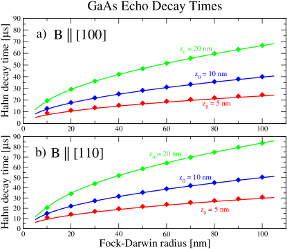
Figure 2: (Color online) Hahn echo total decay times, $t_{0}^{1}=2\tau_{0}^{1}$, for GaAs quantum dots with various Fock-Darwin radii $r_{0}$ and thickness $z_{0}$ comparing the continuum approximation results (solid lines) to $1/e$ decay times obtained via the cluster expansion and previously presented in Ref. witzelHahnLong, . This example includes dipolar but not indirect exchange interactions; it therefore slightly over-estimates the decay time.

IV.4 When is the short-time limit appropriate?

The short-time behavior will be exhibited on a time scale that is short relative to the time scale of the dynamics of the relevant cluster contributions in $\hat{W}^{[1]}$. Because a large number of these cluster contributions are added together in $\operatorname{Re}{\left\{\langle\hat{W}^{[1]}\rangle\right\}}$ [and then exponentiated to yield $v_{E}$ from Eq. (20)], it is possible for the decay of the echo, $v_{E}$, to occur on a time scale that is small relative to the dynamical time scales of any significantly contributing cluster. In particular, the decay will exhibit a short-time behavior when the clusters with the fastest dynamics dominate $\operatorname{Re}{\left\{\langle\hat{W}^{[1]}\rangle\right\}}$. When there is a mixture of dynamical time scales playing a role, then the short-time behavior will be washed out by oscillations generated by HF-induced precessions of the nuclei.

In considering the dynamical time scale of a cluster contribution, we really want to know the effect of this cluster on electron spin dephasing. This is determined by the difference in HF energies (with a reciprocal relationship between time and energy) for different spin polarization configurations of the nuclei in the cluster. In the extreme case that all of the HF energies are the same, there is no spectral diffusion induced (the dynamical time scale is infinite). The dynamical time scale is also determined by the interactions between the nuclei that can cause changes in the spin polarization configurations (turning these interactions off will also shut off spectral diffusion); however, we can estimate a lower bound time scale from just the inverse of differences in HF energies among the cluster.

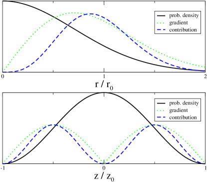
Figure 3: (Color online) A comparison of the position dependence of the electron probability density, absolute value of the gradient of this density [strictly speaking, $\|\frac{\partial}{\partial r}P(\vec{r})\|$ and $\|\frac{\partial}{\partial z}P(\vec{r})\|$ for the top and bottom graphs respectively], and the resulting contribution to the short-time behavior of SD [integrand of Eq. (46) $\propto r\left(\frac{\partial}{\partial r}P(\vec{r})\right)^{2}$ and $\propto\left(\frac{\partial}{\partial z}P(\vec{r})\right)^{2}$ for the top and bottom graphs respectively] for a laterally confined quantum dot of the form of Eq. (48). The curves have arbitrary vertical scales. The short-time behavior exhibited by the SD decay of such quantum dots is related to the fact that the maximum contributions occur roughly where the gradient is maximum and differences in HF coupling among neighboring nuclei are large.

We first address the $\Omega_{e}\rightarrow\infty$ limit and later discuss, briefly, the short-time behavior of HF-mediated interactions. Our previouswitzelHahnShort ; witzelHahnLong ; witzelCPMG results in the $\Omega_{e}\rightarrow\infty$ limit show that the echo decay typically exhibits a short-time behavior in quantum dots with assumed Gaussian shaped wavefunctions but not in donors with exponential-like wavefunctions. This is understood in the following way. In the case of the donor, the fastest dynamics come from those few nuclei in the center that have large differences in HF energies. These are too few in number to dominate the decay; therefore, a mixture of time scales must play a role, slowing down but contributing more as we consider clusters further from the center, and the short-time behavior is washed out. For a quantum dot with a Gaussian shaped wavefunction, however, the fastest contributions occur where the wavefunction gradient is large in a ring around the dot at a radius of the characteristic size of the dot. There are many such clusters that are collectively capable of dominating the echo decay so that it will exhibit a short-time behavior. These arguments are illustrated in Figs. 3 and 4.

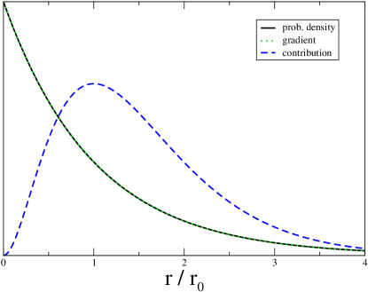
Figure 4: (Color online) A comparison of the position dependence of the electron probability density, absolute value of the gradient of this density, $\|\frac{\partial}{\partial r}P(\vec{r})\|\propto P(\vec{r})$, and the resulting contribution to the short time behavior SD [integrand of Eq. (46) $\propto r^{2}\left(\frac{\partial}{\partial r}P(\vec{r})\right)^{2}$] for an electron with an exponential probability density of the form $P(\vec{r})=\exp(-r/r_{0})$ where $r=\|\vec{r}\|$. Donor bound electrons, such as in Si:P, have an exponential-type decay (though not quite as simple). The curves have arbitrary vertical scales. The failure of the time expansions in such systems is related to the fact that the maximum contributions do not occur where the gradient is maximum.

There is a simple self-consistent check of the short-time behavior [Eqs. (45) and (46)] in the $\Omega_{e}\rightarrow\infty$ limit by comparing $\tau_{0}$ to the fastest dynamical timescale estimated by the maximum gradient multiplied by the lattice spacing (as a typical distance scale between nuclei). Thus, the short-time behavior is valid when $\tau_{0}\ll 1/\left[a\max{\lvert\vec{\nabla}A(\vec{r})\rvert}\right]$. For an electron probability density of the form of Eq. (48), $\max{\lvert\vec{\nabla}A(\vec{r})\rvert}\sim\max{\left(A_{n}/r_{0},A_{n}/z_{0}\right)}$. With $r_{0}\gg z_{0}$, the dynamical time scale has more to do with the position of the cluster in the $z$ direction rather than the radial direction with a time scale estimate of $\tau\sim z_{0}/aA_{n}$. With a $10~{}\mbox{nm}$ quantum dot thickness for $z_{0}$ and lattice constant of about $0.5~{}\mbox{nm}$, this sets a time scale of about $10~{}\mbox{$\mu$s}$. This estimation is slightly pessimistic because we have computed cluster expansion results for $z_{0}=10~{}\mbox{nm}$ and $r_{0}=100~{}\mbox{nm}$ to obtain $\tau_{0}\sim 25~{}\mbox{$\mu$s}$ Hahn echo decay exhibiting the short-time behavior even though $\tau_{0}>10~{}\mbox{$\mu$s}$. However, our $10~{}\mbox{$\mu$s}$ estimate is expected to be overly short because the dynamics is slowed by the weak $10~{}\mbox{ms}$ dipolar coupling (necessarily involved in any decoherence in the $\Omega_{e}\rightarrow\infty$ limit).

This paper is primarily restricted to the $\Omega_{e}\rightarrow\infty$ regime. For the moment, however, let us consider a finite $\Omega_{e}$ and discuss the question of short-time behavior validity with HF-mediated interactions. Because these are nonlocal interactions, differences in HF energies can be as large as the HF energies themselves. This sets a dynamical time scale on the order of $1/A_{n}\sim 1~{}\mbox{$\mu$s}$. Also, the fact that HF-mediated interactions are weak does not help too much in this case because there are $N\gtrsim 10^{5}$ nuclei with which a given nucleus may interact; this yields a strong collective interaction of about $NA_{nm}\sim A_{n}$. In a manner of thinking, on a microsecond time scale, a given nucleus is likely to flip-flop with some other nucleus in the bath through the HF-mediated interaction. On the other hand, flip-flops between nuclei with large differences in HF energies will be suppressed due to HF energy conservation. For this reason, clusters with the fastest dynamics, those with large HF energy differences, will give weak contributions due to energy conservation, while the larger contributors with matching HF energies will have slow dynamics. This leads to a situation similar to that of the donor electron in the $\Omega_{e}\rightarrow\infty$ limit, where the fastest contributors cannot dominate and, therefore, the short-time behavior is washed out. A proper treatment of HF-mediated interactions, therefore, would not use the time perturbation; instead, we should use the intrabath perturbation, perturbatively treating both dipolar and HF-mediated interactions with respect to the HF interaction.

The short-time behavior that we consider in this paper, with its convenient application in the continuum approximation, only applies in the $\Omega_{e}\rightarrow\infty$ limit, where the HF-mediated interactions are negligible. How large does $\Omega_{e}$ need to be for this limit to apply? We may pose this question differently to ask: How does $\Omega_{e}$ affect the time scale of short-time behavior convergence? If we can push this time scale sufficiently larger than $\tau_{0}$, the short-time behavior will emerge. The HF-mediated interaction represents the lowest-order interaction with a magnetic-field dependence, $A_{nm}=A_{n}A_{m}/4\Omega_{e}$. The time scale of the fast dynamics due to the HF-mediated interactions will be a combination of the difference in HF energies ($\sim A_{n}$) and the collective HF-mediated energy ($\sim NA_{nm}$) to give a time scale of $\sim\left(A_{n}NA_{nm}\right)^{-1/2}\propto\sqrt{\Omega_{e}}$. Therefore, according to this simple argument, it is necessary to quadruple $\Omega_{e}$ in order to double the time scale of the short-time behavior as long as HF-mediated interactions are dominant over local internuclear interactions. The lowest-order effects of HF-mediated interactions, however, are reversed by any DD refocusing technique. Therefore, this argument is only relevant for FID.

V Singlet-triplet double quantum dots

Remarkable experiments have recentlypetta05 ; Delft investigated the coherence properties of a single qubit in GaAs quantum dots. In the earlier of these experiments,petta05 the qubit was not the spin of a single electron but, rather, a subspace of two electron spins, each in separate quantum dots with a controllable exchange interaction between the two dots. The qubit states are represented by the two-electron spin states with zero total spin, $\lvert\uparrow\rangle_{1}\otimes\lvert\downarrow\rangle_{2}$ and $\lvert\downarrow\rangle_{1}\otimes\lvert\uparrow\rangle_{2}$, where the $1$ and $2$ subscripts label the dots (and contained electrons). An applied magnetic field protects each electron spin from depolarization; at the same time, the degeneracy of the zero-spin subspace is protected from uniform magnetic-field fluctuations.doubleQDproposal Electrostatic potentials are used to manipulate the electrons. State preparation and final readout are performed by biasing the two electrons, with an applied voltage, into the same dot so that the singlet state, $\left(\lvert\uparrow\rangle_{1}\otimes\lvert\downarrow\rangle_{2}+\lvert\downarrow\rangle_{1}\otimes\lvert\uparrow\rangle_{2}\right)/\sqrt{2}$, has the lowest energy because of the Pauli-exchange interaction.doubleQDproposal ; doubleQD Voltage control is also used to turn on an exchange interaction by allowing the wavefunction of the two electrons on different dots to overlap; such control can be used to rotate the qubit.doubleQDproposal ; doubleQD By using this control, one can apply $\pi$ pulses in order to perform a Hahn echo sequence or any other DD sequence (such as those discussed in Sec. II.3) to prolong the coherence of the qubit.

We can simply map this two-electron qubit into our single-spin qubit formalism. For convenience, we will define $\lvert 0\rangle=\lvert\uparrow\rangle_{1}\otimes\lvert\downarrow\rangle_{2}$ and $\lvert 1\rangle=\lvert\downarrow\rangle_{1}\otimes\lvert\uparrow\rangle_{2}$ as our two qubit basis states. Turning on the exchange interaction will split the energies of the $(\lvert 0\rangle+\lvert 1\rvert)/\sqrt{2}$ and $(\lvert 0\rangle-\lvert 1\rvert)/\sqrt{2}$ superposition states and thereby rotate the qubit in a “transverse” direction as required for a DD sequence that combats dephasing. In order to obtain the free evolution Hamiltonian needed by our formalism, we simply need to derive the qubit-bath Hamiltonian, $\hat{\cal H}_{eb}\hat{S}_{z}$, from the qubit-bath interactions in each of the two dots, $\hat{\cal H}_{eb}^{(1)}\hat{S}_{1z}+\hat{\cal H}_{eb}^{(2)}\hat{S}_{2z}$, by taking its matrix elements in terms of our qubit basis states. With these definitions where we only have a dephasing coupling between the qubit and the bath, it is clear that $\langle 0|\hat{\cal H}_{eb}^{(1)}\hat{S}_{1z}+\hat{\cal H}_{eb}^{(2)}\hat{S}_{2z}|1\rangle=\langle 1|\hat{\cal H}_{eb}^{(1)}\hat{S}_{1z}+\hat{\cal H}_{eb}^{(2)}\hat{S}_{2z}|0\rangle=0$; we thus have only the following dephasing qubit-bath interaction:

$$\hat{\cal H}_{eb} = 2\langle 0|\hat{\cal H}_{eb}^{(1)}\hat{S}_{1z}+{\cal H}_{eb}^{(2)}\hat{S}_{2z}|0\rangle$$ (53a)

$$= -2\langle 1|\hat{\cal H}_{eb}^{(1)}\hat{S}_{1z}+{\cal H}_{eb}^{(2)}\hat{S}_{2z}|1\rangle$$

$$= \hat{\cal H}_{eb}^{(1)}-\hat{\cal H}_{eb}^{(2)}.$$ (53b)

For each dot $i$, the qubit-bath interaction is given by

$$\hat{\cal H}_{eb}^{(i)}=\frac{1}{2}\sum_{n\in\mbox{\scriptsize dot}~{}i}A_{n}^{(i)}I_{nz}+\frac{1}{2}\sum_{n\neq m\in\mbox{\scriptsize dot}~{}i}A_{nm}^{(i)}\hat{I}_{n+}\hat{I}_{m-}.$$ (54)

During the free evolution part of the pulse sequence, the two electrons must essentially have no overlap in their wavefunctions; therefore, $A_{n}^{(i)}$ will only be nonzero when $n$ represents a nucleus in dot $i$. This is the justification for summing over only the relevant dot in Eq. (54).

Assuming that the internuclear interactions occur only within the same bath (and that the bath is initially uncorrelated), then the problem fully decouples into spectral diffusion problems for dots $1$ and $2$ separately. With regards to $\hat{W}^{[1]}$ in the cluster approximation [Eq. (20)], we simply need to sum the cluster contributions in the two dots separately. In a random unpolarized bath with two equivalent dots, the cluster contributions in each dot will be identical; then $v_{E}$ is simply the squared value of the echo for the problem of a single electron in just one of the dots. There should, thus, be no qualitative difference between the spectral diffusion of a single-spin qubit and this double-spin qubit; a prediction of $v_{E}\sim\exp{\left[-(\tau/\tau_{0})^{4}\right]}$ for a single-spin qubit will carry over to the double-spin qubit.

Although the reported Hahn echo decay time $T_{2}$ of Ref. petta05, is compatible with our theory (which disregards other decoherence mechanism) as a limiting case, it is clear that the experimental echo decay does not match the $\exp{\left[-(\tau/\tau_{0})^{4}\right]}$ form. The experimentalists seem to be observing a decoherence mechanism that we are not treating. They report that the $T_{2}$ time increases with an increase in magnetic fieldpetta05 ; therefore, they must not be operating in the high field limit regime. Our results may be viewed as yielding the best decoherence times achievable by increasing the applied magnetic field.

V.1 Dynamic nuclear polarization and the “Zamboni effect”

To minimize the effects of decoherence due to a bath of nuclear spins, one strategy is to polarize the nuclei. When they are polarized, they cannot flip-flop. This is particularly appealing in III-V semiconductors, where all of the isotopes have nonzero spin. Recent experiments have successfully achieved some degree of nuclear polarization in double quantum dot systems.doubleDotNucPolarization This is accomplished by biasing to a point where there is an anticrossing between the single state and the $m_{s}=+1$ triplet state; the transition between these states requires a nuclear spin flip to conserve angular momentum. By cycling through this anticrossing, they are able to produce polarizations of a few percent (producing effective nuclear fields of about $20~{}\mbox{mT}$ in dots where full polarization would yield about $5~{}\mbox{T}$).doubleDotNucPolarization

Even with such modest polarization, there can be a significant impact on inhomogeneous broadening. It does this by effectively smoothing out the hyperfine field and, because of this smoothing, has been coined the Zamboni effect by experimentalists.doubleDotNucPolarization Essentially, the process of dynamic nuclear polarization will most likely polarize those nuclei with the strongest coupling to the electron, those with the largest hyperfine coupling. These nuclei are also the most important in terms of inhomogeneous broadening (they give the largest contribution to the effective magnetic field). Strong polarization is not necessarily involved in the suppression of inhomogeneous broadening. Homogenizing the system to remove the broadening need only change the polarization by roughly the same amount as the unbiased statistical broadening, which scales as $1/\sqrt{N}$; this is less than $1\%$ for $N=10^{5}$. By removing the effects of inhomogeneous broadening in this way, it may be possible to view FID due to SD.

This modest polarization will have a weak effect on SD according to our theory. While $T_{2}^{*}$ (from inhomogeneous broadening) is improved by this strategy, $T_{2}$ (from spectral diffusion) is not significantly altered. There are two reasons for this. First, the nuclei being polarized are not necessarily those nuclei responsible for SD. This is illustrated in Fig. 3 where the regions of electron occupation probability do not correspond to the greatest SD contributors. Second, SD has a weak dependence on polarization because its contributors are clusters of two or more nuclei. Where we quantify polarization as $p=p_{\uparrow}-p_{\downarrow}$ (the difference of the probability of being up versus down assuming spin $1/2$ nuclei), the number of pairs that can flip-flop scales as $(1-p^{2})$.DasSarmaSSC When the spin is larger than $1/2$, the dependence is even weaker (there is a larger fraction of states of two nuclei that can flip-flop). Therefore, one needs nearly $100\%$ polarization in order to suppress SD $T_{2}$ decay.

Therefore, we predict, with substantial confidence, that the coherence enhancement by the Zamboni effect could at best lead to a decoherence time of $T_{I}(\gg T_{2}^{*})$, but never up to $T_{2}(\gtrsim T_{I})$, i.e., the Zamboni effect would never produce a coherence time longer than the spin echo coherence time.

VI Discussion and Conclusion

The main result of this paper is the decoherence time formula of Eq. (46) with wavefunction dependence [Eq. (52) for the specific case of Gaussian-type simple harmonic oscillator confinement]. By using a table (Table 2 for GaAs and InAs) of values for a time quantity we denote by $\mu$, this formula will yield $\tau_{0}^{(l)}$ for a given pulse sequence of $l$ concatenations of the Hahn echo ($l=0$ for free induction decay, and $l=1$ for the Hahn spin echo itself); the initial behavior of the coherence or echo decay is $\exp{(-[\tau/\tau_{0}^{(l)}]^{p(l)})}$ [Eqs. (47) and (31)], where $\tau$ is the time between pulses for the given sequence. By using our definitions of decoherence times, $T_{I}=\tau_{0}^{(0)}$ (free induction decay) and $T_{2}=2\tau_{0}^{(1)}$ (the traditional Hahn echo). The generalized concatenated echo decoherence times are $T_{2}^{(l)}=2^{l}\tau_{0}^{(l)}$. An interesting experimental test of this theory could be to compare the decoherence times of the same sample with an applied magnetic field in different lattice directions and check for agreement with Table 2 (for GaAs or InAs); in such a test, however, one must carefully account for any change in confinement as a result of changes in the applied magnetic field. For experimental systems that allow for the application of pulse sequences, with the ability to perform rapid $\pi$ rotations of the electron spin relative to dynamical time scales, a more straightforward test would be to compare different levels of concatenation and check for agreement with Table 2 and Eqs. (31) and (47).

There are two important approximations that our decoherence time formula assumes. First, we take the limit of a large applied magnetic field. This may not always be experimentally accessible, but, in any case, our results represent the maximum coherence times achievable by applying a strong magnetic field. Second, we use a short-time approximation and discuss its validity in Sec. IV.4. Failure of the short-time approximation does not invalidate our general cluster expansion [Sec. III.1 and Ref. witzelHahnLong, ], however; it only means that our simple wavefunction dependent decoherence time formula [Eq. (46)] is no longer accurate.

Finally, in our considerations of the singlet-triplet (two electron) double quantum dot scenario, we show that it is equivalent to the single dot (one electron) case in terms of spectral diffusion assuming negligible exchange interaction between pulses. (For a treatment that includes the exchange interaction, see Ref. DoubleDotWithExchange, .) We also predict that the Zamboni effect will have little impact upon spectral diffusion.

Appendix A Factorizability of cluster contributions

We define $\hat{W}_{\cal C}^{\prime}$ as the contribution of cluster ${\cal C}$ to $\hat{W}$; that is, $\hat{W}_{\cal C}^{\prime}$ gives the sum of all terms of $\hat{W}^{[1]}$ that involve cluster ${\cal C}$. Thus,

$$\hat{W}^{[1]}=\sum_{{\cal C}\neq\emptyset}\hat{W}_{\cal C}^{\prime}.$$ (55)

Likewise, we will define $\hat{W}_{\cal A,\cal B}^{\prime}$ as the sum of all terms of $\hat{W}^{[2]}$ that involve clusters ${\cal A}$ and ${\cal B}$ so that

$$\hat{W}^{[2]}=\frac{1}{2}\sum_{\begin{subarray}{c}{\cal A},{\cal B}\neq\emptyset\\ {\cal A}\bigcap{\cal B}=\emptyset\end{subarray}}\hat{W}_{\cal A,\cal B}^{\prime},$$ (56)

where the factor of $1/2$ is necessary to compensate for the double counting of $\hat{W}_{\cal B,\cal A}^{\prime}=\hat{W}_{\cal A,\cal B}^{\prime}$ and defining $\hat{W}_{\cal S}$ to be the solution of $\hat{W}$ when only including nuclei in the set ${\cal S}$ (with all of the interactions between them). Similarly, we may define $\hat{W}_{{\cal A},{\cal B}}$ to be the solution of $\hat{W}$ when only including nuclei in the sets ${\cal A}$ and ${\cal B}$ with interactions among ${\cal A}$ and among ${\cal B}$ but not between ${\cal A}$ and ${\cal B}$. Because $\hat{W}_{{\cal A},{\cal B}}$ is just a product of evolution operators of the form $\exp{\left(-i\left[\hat{\cal H}_{\cal A}^{\pm}+\hat{\cal H}_{\cal B}^{\pm}\right]\tau\right)}=\exp{\left(-i\hat{\cal H}_{\cal A}^{\pm}\tau\right)}\exp{\left(-i\hat{\cal H}_{\cal B}^{\pm}\tau\right)}$, $\hat{W}_{{\cal A},{\cal B}}=\hat{W}_{\cal A}\otimes\hat{W}_{\cal B}$. Note that $\hat{W}_{\cal C}^{\prime}$ is the ${\cal C}$ cluster contribution to any $\hat{W}_{\cal S}$ with ${\cal S}\supset{\cal C}$; this is simply due to the fact that any interactions of $\hat{W}$ that are not contained in $\hat{W}_{\cal S}$ are irrelevant when considering terms that do not involve those interactions. For this reason, $\hat{W}_{\cal A}^{\prime}$ is the ${\cal A}$ cluster contribution of $\hat{W}_{{\cal A},{\cal B}}=\hat{W}_{\cal A}\otimes\hat{W}_{\cal B}$ and $\hat{W}_{\cal B}^{\prime}$ is its ${\cal B}$ cluster contribution. Therefore, $\hat{W}_{\cal A,\cal B}^{\prime}=\hat{W}_{\cal A}^{\prime}\otimes\hat{W}_{\cal B}^{\prime}$ so that the double cluster contribution is simply the product of the individual cluster contributions.

This procedure may be applied to terms of any number of clusters so that

$$\hat{W}=\sum_{\begin{subarray}{c}\left\{{\cal C}_{i}\right\}~{}\mbox{\scriptsize{disjoint}},\\ {\cal C}_{i}~{}\neq~{}\emptyset,\end{subarray}}\prod_{\otimes~{}i}\hat{W}_{{\cal C}_{i}}^{\prime}.$$ (57)

Assuming that the initial bath states are uncorrelated, then $\langle\hat{W}_{\cal A}^{\prime}\otimes\hat{W}_{\cal B}^{\prime}\rangle=\langle\hat{W}_{\cal A}^{\prime}\rangle\times\langle\hat{W}_{\cal B}^{\prime}\rangle$ and

$$\langle\hat{W}\rangle=\sum_{\begin{subarray}{c}\left\{{\cal C}_{i}\right\}~{}\mbox{\scriptsize{disjoint}},\\ {\cal C}_{i}~{}\neq~{}\emptyset,\end{subarray}}\prod_{i}\langle\hat{W}_{{\cal C}_{i}}^{\prime}\rangle,$$ (58)

which essentially reproduces our cluster decomposition from Ref. witzelHahnLong, .

When only small clusters, relative to the size of the bath, give non-negligible contributions to $\hat{W}^{[1]}$, then this factorizability allows us to make the following approximation:

$$\langle\hat{W}^{[k]}\rangle\approx\frac{1}{k!}\langle\hat{W}^{[1]}\rangle^{k},$$ (59)

assuming $k\ll N$. The right hand side will provide all necessary products of cluster contributions without overcounting (the $1/k!$ factor compensates for permutation overcounting); however, it also includes products among overlapping clusters. In a large bath, sets of overlapping clusters are negligible compared to the number of sets of nonoverlapping clusters so that these extraneous terms are negligible.

Appendix B Computing the continuum approximation tensor

Computing ${\bf M}^{(l)}$ of Eq. (43) by calculating $f_{b}^{(l)}(\vec{r}_{m})$ from Eq. (34) offers the advantage of simplifications due to the fact that operators which act on different sets of nuclei must commute. For example, to compute $\left[\hat{I}_{nz},{\hat{H}}_{b}\right]$, one need only consider the terms in ${\hat{H}}_{b}$ that involve $m$. For us, however, it was more convenient to reuse a code that computes $\langle\hat{W}_{\cal C}^{\prime}\rangle$ for any set of nuclei, ${\cal C}$. By noting Eqs. (21b) and (IV.2), we may compute $f_{n,n}^{(l)}$ by letting $A_{k}\propto\delta_{n,k}$ and summing together the lowest-order (in the time expansion) results of all cluster contributions, $\langle\hat{W}_{\cal C}^{\prime}\rangle$, that include nucleus $n$ ($n\in{\cal C}$). Similarly, if we let $A_{k}\propto\delta_{n,k}+\delta_{m,k}$ for a given pair $n\neq m$, we may compute $f_{n,n}^{(l)}+f_{m,m}^{(l)}+f_{n,m}^{(l)}+f_{m,n}^{(l)}$. Subtracting off the $f_{n,n}^{(l)}$ and $f_{m,m}^{(l)}$ parts that may be computed by using $A_{k}\propto\delta_{n,k}$ and $A_{k}\propto\delta_{m,k}$, we can obtain $f_{n,m}^{(l)}+f_{m,n}^{(l)}$, which may then be used to compute ${\bf M}^{(l)}$ from Eqs. (43) and (42). We may also use a statistical sampling of clusters to speed up the calculation of ${\bf M}^{(l)}$, which is particularly useful as one increases the number of concatenations, $l$.

References

- (1) A. M. Tyryshkin and S. A. Lyon (private communication); A. M. Tyryshkin, S. A. Lyon, A.V. Astashkin, and A. M. Raitsimring, Phys. Rev. B 68, 193207 (2003); A. M. Tyryshkin, J. J. L. Morton, S. C. Benjamin, A. Ardavan, G. A. D. Briggs, J. W. Ager, and S. A. Lyon, J. Phys.: Condens. Matter 18, S783 (2006).
- (2) E. Abe, K.M. Itoh, J. Isoya and S. Yamasaki, Phys. Rev. B 70, 033204 (2004); E. Abe, A. Fujimoto, J. Isoya, S. Yamasaki and K.M. Itoh, arXiv:cond-mat/0512404 (unpublished).
- (3) J. R. Petta (private communication); J.R. Petta, A. C. Johnson, J. M. Taylor, E. A. Laird, A. Yacoby, M. D. Lukin, C. M. Marcus, M. P. Hanson, and A. C. Gossard, Science 309, 2180 (2005).
- (4) F. H. L. Koppens, J. A. Folk, J. M. Elzerman, R. Hanson, L. H. Willems van Beveren, I. T. Vink, H. P. Tranitz, W. Wegscheider, L. P. Kouwenhoven, and L. M. K. Vandersypen, Science 309, 1346 (2005); R. Hanson, L. H. Willems van Beveren, I. T. Vink, J. M. Elzerman, W. J. M. Naber, F. H. L. Koppens, L. P. Kouwenhoven, and L. M. K. Vandersypen, Phys. Rev. Lett. 94, 196802 (2005); F. H. L. Koppens, K. C. Nowack, and L. M. K. Vandersypen, arXiv:0711.0479 (unpublished).
- (5) A. Greilich, D. R. Yakovlev, A. Shabaev, Al. L. Efros, I. A. Yugova, R. Oulton, V. Stavarache, D. Reuter, A. Wieck, and M. Bayer, Science 313, 341 (2006).
- (6) R. de Sousa and S. Das Sarma, Phys. Rev. B 68, 115322 (2003).
- (7) D. Klauser, W. A. Coish, and D. Loss, Adv. Solid State Phys. 46, 17 (2007). W. A. Coish and D. Loss, Phys. Rev. B 70, 195340 (2004).
- (8) W. M. Witzel, R. de Sousa, and S. Das Sarma, Phys. Rev. B 72, 161306(R) (2005).
- (9) Wang Yao, Ren-Bao Liu, and L. J. Sham, Phys. Rev. B 74, 195301 (2006).
- (10) C. Deng and X. Hu, Phys. Rev. B 73 241303(R) (2006); arXiv:cond-mat/0608544 (unpublished).
- (11) W. M. Witzel and S. Das Sarma, Phys. Rev. B 74, 035322 (2006).
- (12) W. M. Witzel and S. Das Sarma, Phys. Rev. Lett. 98, 077601 (2007).
- (13) Wang Yao, Ren-Bao Liu, and L. J. Sham, Phys. Rev. Lett. 98, 077602 (2007).
- (14) Ren-Bao Liu, Wang Yao, and L. J. Sham, New J. Phys. 9, 226 (2007).
- (15) W. M. Witzel and S. Das Sarma, Phys. Rev. B 76, 241303(R) (2007).
- (16) B. Lee, W. M. Witzel, and S. Das Sarma, arXiv:0710.1416 (accepted to Phys. Rev. Lett.).
- (17) Götz S. Uhrig, Phys. Rev. Lett. 98, 100504 (2007).
- (18) B. Herzog and E. L. Hahn, Phys. Rev. 103, 148 (1956); A. M. Portis, ibid. 104, 584 (1956).
- (19) G. Feher and E. A. Gere, Phys. Rev. 114, 1245 (1959).
- (20) W. B. Mims and K. Nassau, Bull. Am. Phys. Soc. 5, 419 (1960); W. B. Mims, K. Nassau, and J. D. McGee, Phys. Rev. 123, 2059 (1961).
- (21) J. R. Klauder and P. W. Anderson, Phys. Rev. 125, 912 (1962).
- (22) G. M. Zhidomirov and K. M. Salikhov, Sov. Phys. JETP 29, 1037 (1969).
- (23) M. Chiba and A. Hirai, J. Phys. Soc. Jpn. 33, 730 (1972).
- (24) S. K. Saikin, Wang Yao, and L. J. Sham, Phys. Rev. B 75, 125314 (2007).
- (25) R. de Sousa and S. Das Sarma, Phys. Rev. B 67, 033301 (2003).
- (26) R. F. Shulman, J. M. Mays, and D. W. McCall, Phys. Rev. 100, 692 (1955).
- (27) R. F. Shulman, B. J. Wyluda, and H. J. Hrostowski, Phys. Rev. 109, 808 (1958).
- (28) R. K. Sundfors, Phys. Rev. 185, 458 (1969).
- (29) W. M. Witzel, Xuedong Hu, S. Das Sarma, Phys. Rev. B 76, 035212 (2007).
- (30) R. Winkler, Spin-Orbit Coupling Effects in Two-Dimensional Electron and Hole Systems (Springer-Verlag, Berlin, 2003), Appendix B.
- (31) C. P. Slichter, Principles of Magnetic Resonance, 3rd ed. (Springer-Verlag, Berlin, 1990).
- (32) N. Bloembergen and T. J. Rowland, Phys. Rev. 97, 1679 (1955).
- (33) N. Shenvi, R. de Sousa, and K. B. Whaley, Phys. Rev. B 71, 224411 (2005).
- (34) A. Abragam, The Principles of Nuclear Magnetism (Oxford University Press, London, 1961), Chap. IV, Eq. (63).
- (35) P. W. Anderson, Phys. Rev. 99, 623 (1955).
- (36) K. Khodjasteh and D. A. Lidar, Phys. Rev. A. 75, 062310 (2007).
- (37) W. Magnus, Commun. Pure Appl. Math. 7, 649 (1954).
- (38) L. Viola and E. Knill, Phys. Rev. Lett. 94, 060502 (2005).
- (39) K. Khodjasteh and D.A. Lidar, Phys. Rev. Lett. 95, 180501 (2005).
- (40) H. Y. Carr and E. M. Purcell, Phys. Rev. 94, 630 (1954); S. Meiboom and D. Gill, Rev. Sci. Instrum. 29, 6881 (1958).
- (41) C. Kittel, Introduction to Solid State Physics, 7th ed. (Wiley, New York, 1996).
- (42) CRC Handbook of Chemistry and Physics, 70th ed., E-82 (CRC, Boca Raton, FL, 1989).
- (43) Encyclopedia of Nuclear Magnetic Resonance, D. M. Granty and R. K. Harris, (eds.), vol. 5, John Wiley & Sons, Chichester, UK, 1996.
- (44) D. Paget, G. Lampel, B. Sapoval, and V. I. Safarov, Phys. Rev. B 15, 5780 (1977).
- (45) J. M. Taylor, H.-A. Engel, W. Dur, A. Yacoby, C. M. Marcus, P. Zoller, and M. D. Lukin, Nat. Phys. 1, 177 (2005).
- (46) J. R. Petta, A. C. Johnson, J. M. Taylor, A. Yacoby, M. D. Lukin, C. M. Marcus, M. P. Hanson, and A. C. Gossard, Physica E (Amsterdam) 34, 42 (2006); E. A. Laird, J. R. Petta, A. C. Johnson, C. M. Marcus, A. Yacoby, M. P. Hanson, and A. C. Gossard, Phys. Rev. Lett. 97, 056801 (2006); J. M. Taylor, J. R. Petta, A. C. Johnson, A. Yacoby, C. M. Marcus, and M. D. Lukin, Phys. Rev. B 76, 035315 (2007).
- (47) J. R. Petta, J. M. Taylor, A. C. Johnson, A. Yacoby, M. D. Lukin, C. M. Marcus, M. P. Hanson, and A. C. Gossard, Phys. Rev. Lett. 100, 067601 (2008); C. M. Marcus (private communication).
- (48) S. Das Sarma, Rogerio de Sousa, Xuedong Hu, and Belita Koiller, Solid State Commun. 133, 737 (2005).
- (49) W. Yang and R. B. Liu, Phys. Rev. B 77, 085302 (2008).