Spectral Flow in AdS${}_{3}/$CFT₂

Abstract:

We study the spectral flowed sectors of the 3 WZW model in the context of the holographic duality between type IIB string theory in $AdS_{3}\times S^{3}\times T^{4}$ with NSNS flux and the symmetric product orbifold of $T^{4}$. We construct explicitly the physical vertex operators in the flowed sectors that belong to short representations of the superalgebra, thus completing the bulk-to-boundary dictionary for 1/2 BPS states. We perform a partial calculation of the string three-point functions of these operators. A complete calculation would require the three-point couplings of non-extremal flowed operators in the 3 WZW model, which are at present unavailable. In the unflowed sector, perfect agreement has recently been found between the bulk and boundary three-point functions of 1/2 BPS operators. Assuming that this agreement persists in the flowed sectors, we determine certain unknown three-point couplings in the 3 WZW model in terms of three-point couplings of affine descendants in the $SU(2)$ WZW model.

1 Introduction

A classic example of the AdS/CFT correspondence is the duality between type IIB string theory on $AdS_{3}\times S^{3}\times M^{4}$, where $M^{4}$ is hyperkähler, and a certain deformation of Sym${}^{N}(M^{4})$, the symmetric product orbifold of $N$ copies of $M^{4}$ [1]. The duality can be motivated from the near-horizon limit of a system of $Q_{5}$ D5-branes and $Q_{1}$ D1-branes, or, in the S-dual frame, of $Q_{5}$ NS5 branes and $Q_{1}$ fundamental strings. The number $N$ of copies of $M^{4}$ entering the symmetric product is given by $N=Q_{1}Q_{5}$.

While several aspects of this duality were understood early on (see e.g. [2, 3, 4, 5] for reviews), only this year has the status of correlation functions become more clear. Three-point functions of 1/2 BPS operators have been obtained on the string side through exact worldsheet computations [6, 7, 8], and found to be in precise agreement with the boundary results of [9, 10, 11]. Previous supergravity computations [12, 13, 14], which appeared to show a discrepancy, have then been revisited [15] and found to be compatible with this perfect agreement once a more general ansatz for the bulk-to-boundary dictionary is assumed.

The string theory and the boundary computations are performed at different points in the moduli space [16, 17], where solvable descriptions are available. This strongly suggests the existence of a new non-renormalization theorem. In the boundary, the solvable point is the orbifold Sym${}^{N}(M^{4})$. In the bulk, it is near horizon geometry of the NS5 F1 system, which is $AdS_{3}\times S^{3}\times M^{4}$ with only NSNS flux in the $AdS_{3}\times S^{3}$ factors [18]. This leads to an exact worldsheet description in the RNS formalism in terms of $SL(2,R)_{k+2}$ and $SU(2)_{k-2}$ current algebras, where $k\equiv Q_{5}$, plus some free fermions [19, 20]. In this setting the superconformal invariance of the dual theory can be seen to arise from the string worldsheet [19, 21, 22].

Let us recall the basics of the bulk-to-boundary dictionary for 1/2 BPS operators. The six-dimensional string coupling constant is

$$g_{6}^{2}=\frac{Q_{5}}{Q_{1}}\,,$$ (1)

so string perturbation theory is valid for $Q_{1}\rightarrow\infty$, or $N=Q_{1}Q_{5}\gg Q_{5}$. In this limit, single string states in the bulk map to twisted states in Sym${}^{N}(M^{4})$ associated to conjugacy classes with a single non-trivial cycle. The length $n$ of this cycle is related to the $SL(2,R)$ spin $h$ appearing in the worldsheet vertex operator as

$$n=2h-1\,.$$ (2)

The analysis of [6, 7, 8] included only operators arising from the usual “unflowed” representations of the $SL(2,R)$ current algebra, whose spin is bounded as $h\leq k/2$. On the other hand, the symmetric product orbifold contains cycles of lengh $n\leq N$. So in the large $N$ limit, where the worldsheet description is valid, it appears that infinitely many 1/2 BPS operators are missing in the bulk. The resolution of this puzzle has been known for some time: the additional operators arise [23, 24] from the spectral flowed sectors of the $SL(2,R)$ current algebra [25, 26, 27]. Once spectral flowed representations are included, relation (2) is generalized to

$$n=2h-1+kw\,,\qquad\qquad h=1\,,\frac{3}{2}\,,\ldots\frac{k}{2}\,,\qquad w=0\,,1\,,2\,,\ldots$$ (3)

where $w$ is the spectral flow parameter.

In this paper we give a precise construction of the 1/2 BPS vertex operators in the flowed sectors, thus completing the bulk-to-boundary dictionary, and we study their three-point functions. The physical states in the flowed sectors are the $AdS_{3}$ analogs of what in flat space are the infinite higher-spin string modes – they are genuine string states not visible in supergravity. Indeed, supergravity becomes a good description for $k\to\infty$, and in this limit the flowed states acquire infinite conformal dimension. The BPS condition correlates the $SL(2,R)$ and $SU(2)$ quantum numbers, and the complete vertex operators involve a precise combination of states from the $SU(2)$ WZW model and the worldsheet fermions, which are current algebra descendants but Virasoro primaries.

As in [7], we obtain the vertex operators in the “$x$-basis”, which greatly facilitates explicit computations. We then perform a partial calculation of three-point functions of flowed operators. Some features of the calculation suggest that the agreement with the boundary results continues to hold in the flowed sectors. Unfortunately, a complete calculation requires certain three-point couplings in the $H_{3}^{+}$ WZW model that are not yet available in the CFT literature. We leave their evaluation for future work. Instead of a complete verification of the bulk-to-boundary agreement, we turn the logic around and obtain non-trivial holographic predictions in the form of identities involving three-point couplings of flowed operators of the $H_{3}^{+}$ WZW model and of affine descendants of the $SU(2)$ WZW model.

The organization of the paper is as follows. In Section 2 we review the spectrum and three-point functions of 1/2 BPS operators in the boundary theory, and the spectrum and three-point functions of unflowed 1/2 BPS operators in the the bulk theory. In Section 3, we review the spectral flow in the $SL(2,R)$ affine algebra and study its $SU(2)$ counterpart, which maps current algebra primaries to descendants. In Section 4, we study how the spectral flow organizes the spectrum of the free fermions into $SL(2,R)$ and $SU(2)$ multiplets of Virasoro primaries, and compute their three-point functions. In Section 5 we assemble our previous results to build the flowed 1/2 BPS physical vertex operators. In Section 6 we study their three-point functions and obtain the identities that must hold assuming the bulk-to-boundary agreement. We conclude in Section 7.

2 Review of 1/2 BPS operators and their three-point functions

2.1 The symmetric product orbifold

In this subsection we briefly review the ${\cal N}=2$ and ${\cal N}=4$ spectrum and three-point correlators of the symmetric product orbifold Sym${}^{N}(M^{4})$. For more details see [32, 9, 10, 11].

There is one twisted sector for each conjugacy class of the symmetric group $S_{N}$, given by disjoint cycles of lengths $n_{i}$ and multiplicities $N_{i}$,

$$(n_{1})^{N_{1}}(n_{2})^{N_{2}}\ldots(n_{r})^{N_{r}}\,,\qquad\sum_{i}n_{i}N_{i}=N\,.$$ (4)

According to the AdS/CFT dictionary, in the large $N$ limit each cycle is interpreted as a single string state. Therefore, the chiral primary operators that we are interested in are given by twist fields associated to single cycles of length $n_{i}$, dressed by chiral fields of $M^{4}$ itself, summed in a $S_{N}$ invariant way. For $M^{4}=T^{4}$, the holomorphic chiral fields are $1$, $\psi^{a}\,(a=1,2)$ and $\psi^{1}\psi^{2}$, where $\psi^{1}$ and $\psi^{2}$ are complex fermions formed by grouping the four fermions of $T^{4}$ into two pairs. We will label the chiral operators dressed by $1$, $\psi^{a}$ and $\psi^{1}\psi^{2}$ respectively as $O_{n}^{-},O_{n}^{a}$ and $O_{n}^{+}$. Their holomorphic conformal dimensions are respectively $\Delta=\frac{n-1}{2},\frac{n}{2}$ and $\frac{n+1}{2}$. Each operator has also an independent anti-holomorphic dressing, so the full operators are denoted as $O_{n}^{(\epsilon,{\bar{\epsilon}})}$, where $\epsilon,{\bar{\epsilon}}=-,a,+$.

These operators are ${\cal N}=2$ chiral, namely their conformal dimension $\Delta$ and $U(1)$ R-charge $Q$ satisfy $\Delta=Q/2$. Since Sym${}^{N}(M^{4})$ has ${\cal N}=4$ superconformal symmetry, with affine left and right $SU(2)_{N}$ R-symmetries, these are actually the highest weight states in $SU(2)\times SU(2)$ multiplets of spins $J=\Delta$ and $\bar{J}=\bar{\Delta}$. Denoting the elements of these multiplets as ${\mathbb{V}}_{n,M,{\bar{M}}}^{(\epsilon,{\bar{\epsilon}})}$, we have

$$O_{n}^{(\epsilon,{\bar{\epsilon}})} = {\mathbb{V}}_{n,J,{\bar{J}}}^{(\epsilon,{\bar{\epsilon}})}\,,$$ (5)

$$O_{n}^{(\epsilon,{\bar{\epsilon}})\,\dagger} = {\mathbb{V}}_{n,-J,-{\bar{J}}}^{(\epsilon,{\bar{\epsilon}})}\,,\qquad\epsilon,{\bar{\epsilon}}=-,a,+\,\,.$$ (6)

It is convenient to normalize the modes ${\mathbb{V}}_{n,M,{\bar{M}}}^{(\epsilon,{\bar{\epsilon}})}$ as

$$\langle{\mathbb{V}}_{n,M,{\bar{M}}}^{(\epsilon,{\bar{\epsilon}})}{\mathbb{V}}_{n^{\prime},M^{\prime},{\bar{M}}^{\prime}}^{(\epsilon^{\prime},{\bar{\epsilon}}^{\prime})}\rangle=(-1)^{J+{\bar{J}}-M-{\bar{M}}}\delta_{nn^{\prime}}\delta^{\epsilon\epsilon^{\prime}}\delta^{{\bar{\epsilon}}{\bar{\epsilon}}^{\prime}}\delta_{MM^{\prime}}\delta_{{\bar{M}}{\bar{M}}^{\prime}}\,.$$ (7)

We then sum over formal isospin variables $y,\bar{y}$ to define

$${\mathbb{O}}_{n}^{(\epsilon,{\bar{\epsilon}})}(y,\bar{y})=\sum_{M=-J}^{J}\sum_{{\bar{M}}=-{\bar{J}}}^{{\bar{J}}}\left(c_{M}^{J}c_{{\bar{M}}}^{{\bar{J}}}\right)^{\nicefrac{{1}}{{2}}}\times y^{-M+J}\bar{y}^{-\!{\bar{M}}+{\bar{J}}}{\mathbb{V}}_{n,M,{\bar{M}}}^{(\epsilon,{\bar{\epsilon}})}$$ (8)

where

$$c_{M}^{J}=\left(\begin{array}[]{c}2J\\ M+J\end{array}\right)=\frac{(2J)!}{(J+M)!(J-M)!}\,.$$ (11)

The operators ${\mathbb{O}}_{n}^{(\epsilon,{\bar{\epsilon}})}$ obey

$$\langle{\mathbb{O}}_{n}^{(\epsilon,{\bar{\epsilon}})}\mathbb{O}_{n^{\prime}}^{(\epsilon^{\prime},{\bar{\epsilon}}^{\prime})}\rangle=(y_{1}-y_{2})^{2J}(\bar{y}_{1}-\bar{y}_{2})^{2\bar{J}}\delta_{nn^{\prime}}\delta^{\epsilon\epsilon^{\prime}}\delta^{{\bar{\epsilon}}{\bar{\epsilon}}^{\prime}}\,.$$ (12)

In summary, there are three series of holomorphic $SU(2)$ multiplets ${\mathbb{O}}_{n}^{(-)}(y),{\mathbb{O}}_{n}^{(a)}(y)$ and ${\mathbb{O}}_{n}^{(+)}(y)$, with $\Delta=J=\frac{n-1}{2},\frac{n}{2}$ and $\frac{n+1}{2}$, respectively, where $n=1,\ldots,N$. Similarly, there are three series of antiholomorphic multiplets that depend on the $\bar{y}$ isospin variable. The full 1/2 BPS spectrum is obtained by putting together holomorphic and antiholomorphic multiplets, with the constraint that cycle length $n$ be the same for the holomorphic and antiholomorphic factors.

Extremal $N=2$ correlators

The three-point functions for the ${\cal N}=2$ primaries $O_{n}^{(\epsilon,{\bar{\epsilon}})}$, which correspond to “extremal” correlators in the terminology of [33], were computed in [9]. The fusion rules, obtained from conservation of the $U(1)$ R-charge and the group composition law of the cyclic permutations, are,

$$\begin{array}[]{rclclcr}(-)&\times&(-)&\rightarrow&(-)&+&(+)\\ (-)&\times&(+)&\rightarrow&(+)&&\\ (-)&\times&(\,a\,)&\rightarrow&(\,a\,)&&\\ (\,a\,)&\times&(\,a\,)&\rightarrow&(+)&&\end{array}$$ (17)

both for the holomorphic and the anti-holomorphic sectors. These fusion rules are combined freely between both sectors, except for the process

$$(-)\times(-)\rightarrow(+)$$ (18)

which should occur simultaneously in the left and the right movers. This gives a total combination of $4\times 4+1=17$ possible fusions. In the large $N$ limit, the structure constants for the scalar $(\Delta=\bar{\Delta})$ sector are

$$\langle O_{n_{3}}^{(-,-)\,\dagger}O_{n_{2}}^{(-,-)}O_{n_{1}}^{(-,-)}\rangle = \left(\frac{1}{N}\right)^{1/2}\,\left(\frac{n_{3}^{3}}{n_{1}n_{2}}\right)^{1/2}$$ (19)

$$\langle O_{n_{3}}^{(+,+)\,\dagger}O_{n_{2}}^{(-,-)}O_{n_{1}}^{(-,-)}\rangle = \left(\frac{1}{N}\right)^{1/2}\left(\frac{1}{n_{1}n_{2}n_{3}}\right)^{1/2}$$ (20)

$$\langle O_{n_{3}}^{(+,+)\,\dagger}O_{n_{2}}^{(-,-)}O_{n_{1}}^{(+,+)}\rangle = \left(\frac{1}{N}\right)^{1/2}\left(\frac{n_{1}^{3}}{n_{2}n_{3}}\right)^{1/2}$$ (21)

$$\langle O_{n_{3}}^{(\,a,\bar{a}\,)\,\dagger}O_{n_{2}}^{(\,b,\bar{b}\,)}O_{n_{1}}^{(-,-)}\rangle = \left(\frac{1}{N}\right)^{1/2}\left(\frac{n_{2}n_{3}}{n_{1}}\right)^{1/2}\delta^{ab}\delta^{\bar{a}\bar{b}}$$ (22)

$$\langle O_{n_{3}}^{(+,+)\,\dagger}O_{n_{2}}^{(\,a,\bar{a}\,)}O_{n_{1}}^{(\,b,\bar{b}\,)}\rangle = \left(\frac{1}{N}\right)^{1/2}\left(\frac{n_{1}n_{2}}{n_{3}}\right)^{1/2}\xi^{a\,b}\xi^{\bar{a}\,\bar{b}}\,,$$ (23)

with

$$\xi = \left(\begin{array}[]{rr}0&1\\ 1&0\end{array}\right)\,.$$ (26)

Here $n_{3}$ is fixed in terms of $n_{1}$ and $n_{2}$ from the conservation of $U(1)$ R-charge, which gives  $n_{3}=n_{1}+n_{2}-3$ for (20) and by $n_{3}=n_{1}+n_{2}-1$ for the other cases. The structure constants are actually completely factorized between left and right movers, so for non-scalar operators the three-point functions are products of square roots of the above correlators.

Non-extremal $N=4$ correlators

Correlators involving the elements of the full $SU(2)$ multiplet were computed, in [10, 11], only for operators of type $\epsilon,{\bar{\epsilon}}=\pm$. The fusion rules are

$$n_{i}\leq n_{j}+n_{k}-1\,,\qquad\qquad i\neq j\neq k\qquad i,j,k=1,2,3\,.$$ (27)

Their three-point functions are, in the large $N$ limit,

$$\langle{\mathbb{V}}_{n_{1},M_{1},{\bar{M}}_{1}}^{(\epsilon_{1},{\bar{\epsilon}}_{1})}{\mathbb{V}}_{n_{2},M_{2},{\bar{M}}_{2}}^{(\epsilon_{2},{\bar{\epsilon}}_{2})}{\mathbb{V}}_{n_{3},M_{3},{\bar{M}}_{3}}^{(\epsilon_{3},{\bar{\epsilon}}_{3})}\rangle=\frac{1}{\sqrt{N}}\frac{(\epsilon_{1}n_{1}+\epsilon_{2}n_{2}+\epsilon_{3}n_{3}+1)({\bar{\epsilon}}_{1}n_{1}+{\bar{\epsilon}}_{2}n_{2}+{\bar{\epsilon}}_{3}n_{3}+1)}{4(n_{1}n_{2}n_{3})^{\nicefrac{{1}}{{2}}}}$$ (28)

$$\times L(J_{i},M_{i})L({\bar{J}}_{i},{\bar{M}}_{i})\,\delta_{M_{1}+M_{2}+M_{3},0}\delta_{{\bar{M}}_{1}+{\bar{M}}_{2}+{\bar{M}}_{3},0}\,,$$

where $L(J_{i},M_{i})$ is defined in terms of the $SU(2)$ $3j$ symbols as

$$L(J_{i},M_{i})=\left(\begin{array}[]{ccc}J_{1}&J_{2}&J_{3}\\ M_{1}&M_{2}&M_{3}\end{array}\right)\times\left[\frac{(J_{1}+J_{2}-J_{3})!(J_{2}+J_{3}-J_{1})!(J_{3}+J_{1}-J_{2})!(J_{1}+J_{2}+J_{3}+1)!}{(2J_{1})!(2J_{2})!(2J_{3})!}\right]^{\nicefrac{{1}}{{2}}}\,.$$ (31)

In terms of the ${\mathbb{O}}_{n}^{(\epsilon,{\bar{\epsilon}})}$ multiplets defined in (8), the three-point functions take the simple form [8]

$$\langle{\mathbb{O}}_{n_{1}}^{(\epsilon_{1},{\bar{\epsilon}}_{1})}{\mathbb{O}}_{n_{2}}^{(\epsilon_{2},{\bar{\epsilon}}_{2})}{\mathbb{O}}_{n_{3}}^{(\epsilon_{3},{\bar{\epsilon}}_{3})}\rangle=\frac{1}{\sqrt{N}}\frac{(\epsilon_{1}n_{1}+\epsilon_{2}n_{2}+\epsilon_{3}n_{3}+1)({\bar{\epsilon}}_{1}n_{1}+{\bar{\epsilon}}_{2}n_{2}+{\bar{\epsilon}}_{3}n_{3}+1)}{4(n_{1}n_{2}n_{3})^{\nicefrac{{1}}{{2}}}}$$ (32)

$$\times\,\,y_{12}^{J_{1}+J_{2}-J_{3}}y_{23}^{J_{2}+J_{3}-J_{1}}y_{31}^{J_{3}+J_{1}-J_{2}}\times\,\,\bar{y}_{12}^{\bar{J}_{1}+\bar{J}_{2}-\bar{J}_{3}}\bar{y}_{23}^{\bar{J}_{2}+\bar{J}_{3}-\bar{J}_{1}}\bar{y}_{31}^{\bar{J}_{3}+\bar{J}_{1}-\bar{J}_{2}}\,.$$

One can easily verify that these $N=4$ correlators reduce to the extremal $N=2$ correlators when we specialize to $M_{i}=\pm J_{i}$ and ${\bar{M}}_{i}=\pm\bar{J}_{i}$.

2.2 The $AdS_{3}\times S^{3}\times T^{4}$ worldsheet

In the frame with only NSNS flux, the string background is described by a product of supersymmetric $SL(2,R)$ and $SU(2)$ WZW models at level $k$, which correspond to the $AdS_{3}\times S^{3}$ geometry [18, 19, 20], and four real bosons and fermions, corresponding to the $T^{4}$ factor. We will actually consider the Euclidean form of $AdS_{3}$, where the $SL(2,R)$ WZW model is replaced by the $H_{3}^{+}$ WZW model, and whose affine symmetries are still two copies of $SL(2,R)$.

The supersymmetric affine $SL(2,R)_{k}$ symmetry is generated by the supercurrents $\psi^{A}+\theta J^{A}$, $A=1,2,3$. The OPEs are

$$J^{A}(z)J^{B}(w)\sim {{k\over 2}\eta^{AB}\over(z-w)^{2}}+{i\epsilon^{AB}{}_{C}J^{C}(w)\over z-w}~{},$$ (33)

$$J^{A}(z)\psi^{B}(w)\sim {i\epsilon^{AB}{}_{C}\psi^{C}(w)\over z-w}~{},$$ (34)

$$\psi^{A}(z)\psi^{B}(w)\sim {{k\over 2}\eta^{AB}\over z-w}~{},$$ (35)

where $\epsilon^{123}=1$ and capital letter indices are raised and lowered with $\eta^{AB}=\eta_{AB}=(++-)$. Similarly, the supersymmetric affine $SU(2)_{k}$ symmetry has supercurrents $\chi^{a}+\theta K^{a}$, $a=1,2,3$, with OPEs

$$K^{a}(z)K^{b}(w)\sim {{k\over 2}\delta^{ab}\over(z-w)^{2}}+{i\epsilon^{ab}{}_{c}K^{c}(w)\over z-w}~{},$$ (36)

$$K^{a}(z)\chi^{b}(w)\sim {i\epsilon^{ab}{}_{c}\chi^{c}(w)\over z-w}~{},$$ (37)

$$\chi^{a}(z)\chi^{b}(w)\sim {{k\over 2}\delta^{ab}\over z-w}~{},$$ (38)

and lower case indices are raised and lowered with $\delta^{ab}=\delta_{ab}=(+,+,+)$. We will often use the linear combinations

$$J^{\pm} \equiv J^{1}\pm iJ^{2}\qquad\qquad\psi^{\pm}\equiv\psi^{1}\pm i\psi^{2}\,,$$ (39)

$$K^{\pm} \equiv K^{1}\pm iK^{2}\qquad\qquad\!\!\!\chi^{\pm}\equiv\chi^{1}\pm i\chi^{2}\,.$$ (40)

As usual in supersymmetric WZW models, it is convenient to split the $J^{A},K^{a}$ currents into

$$J^{A} = j^{A}+\hat{\jmath}^{A}\,,$$ (41)

$$K^{a} = k^{a}+\hat{k}^{a}\,,$$ (42)

where

$$\hat{\jmath}^{A} = -\frac{i}{k}\epsilon^{A}{}_{BC}\psi^{B}\psi^{C}\,,$$ (43)

$$\hat{k}^{a} = -\frac{i}{k}\epsilon^{a}{}_{bc}\chi^{b}\chi^{c}\,.$$ (44)

The currents $j^{A}$ and $k^{a}$ generate bosonic $SL(2,R)_{k+2}$ and $SU(2)_{k-2}$ affine algebras, and commute with the free fermions $\psi^{A},\chi^{a}$. The latter in turn form a pair of supersymmetric $SL(2,R)$ and $SU(2)$ models at levels -2 and +2, whose bosonic currents are $\hat{\jmath}^{A}$ and $\hat{k}^{a}$. The spectrum and the interactions of the original level $k$ supersymmetric WZW models are factorized into the bosonic WZW models and the free fermions [34]. In terms of the split currents, the stress tensor and supercurrent of $SL(2,R)$ are

$$T^{H} = \frac{1}{k}j^{A}j_{A}-\frac{1}{k}\psi^{A}{\partial}\psi_{A}\,,$$ (45)

$$G^{H} = \frac{2}{k}(\psi^{A}j_{A}+\frac{2i}{k}\psi^{1}\psi^{2}\psi^{3})\,,$$ (46)

and those of $SU(2)$ are

$$T^{S} = \frac{1}{k}k^{a}k_{a}-\frac{1}{k}\chi^{a}{\partial}\chi_{a}\,,$$ (47)

$$G^{S} = \frac{2}{k}(\chi^{a}k_{a}-\frac{2i}{k}\chi^{1}\chi^{2}\chi^{3})\,.$$ (48)

The total stress tensor and supercurrent are

$$T = T^{H}+T^{S}+T(T^{4})$$ (49)

$$G = G^{H}+G^{S}+G(T^{4})$$ (50)

where $T(T^{4})$ and $G(T^{4})$ are the stress tensor and supercurrent of $T^{4}$, and one can check that the central charge adds up to $c=15$. Here and below we focus on the holomorphic part of the theory, but there is a similar antiholomorphic copy.

A primary field of spin $h$ in the $SL(2,R)_{k+2}$ WZW model satisfies

$$j^{A}(z)\Phi_{h}(x,w)\sim-\frac{D_{x}^{A}\Phi_{h}(x,\bar{x};w,\bar{w})}{z-w}\,,$$ (51)

where the operators $D_{x}^{A}$ are

$$D_{x}^{-} = {\partial}_{x}\,,$$ (52)

$$D_{x}^{3} = x{\partial}_{x}+h\,,$$ (53)

$$D_{x}^{+} = x^{2}{\partial}_{x}+2hx\,.$$ (54)

The conformal dimension of $\Phi_{h}$ is

$$\Delta_{h}=-\frac{h(h-1)}{k}\,.$$ (55)

The field $\Phi_{h}$ can be expanded in modes as

$$\Phi_{h}(x,\bar{x})=\sum_{m,\bar{m}}\Phi_{h,m,\bar{m}}x^{-h-m}\bar{x}^{-h-\bar{m}}\,,$$ (56)

but the range of the summation is not always well defined [20]. Yet, the action of the zero modes of the currents on $\Phi_{h,m,\bar{m}}$ is well defined and can be read from (51) to be

$$j^{3}_{0}\Phi_{h,m,\bar{m}} = m\Phi_{h,m,\bar{m}}\,\,\,\,,$$ (57)

$$j^{\pm}_{0}\Phi_{h,m,\bar{m}} = (m\mp(h-1))\Phi_{h,m\pm 1,\bar{m}}\,\,\,\,,$$ (58)

and similarly for the anti-holomorphic currents. The $x,\bar{x}$ variables are interpreted as the local coordinates of the two-dimensional conformal field theory living in the boundary of $AdS_{3}$.

The Hilbert space of the $SL(2,R)_{k+2}$ consists of the usual “unflowed” sector and of the spectral flowed sectors [25, 26]. Let us recall the structure of the unflowed sector. As usual, we can decompose it in representations of the current algebra built by the action of the negative modes of $j^{A}$ on affine primaries. In turn, the affine primaries form representations of the $SL(2,R)$ algebra of the zero modes. The relevant representations of the zero modes are delta-normalizable continuous representations, with $h=\frac{1}{2}+i\mathbb{R}$ and $m=\alpha+\mathbb{Z}\,(\alpha\in[0,1))$, and non-normalizable discrete representations, with $h\in\mathbb{R}$ obeying

$$\frac{1}{2}<h<\frac{k+1}{2}\,.$$ (59)

The discrete representations can be either lowest-weight $d^{+}_{h}$, with $m=h,h+1\ldots$, or highest-weight $d^{-}_{h}$, with $m=-h,-h-1\ldots$. The spectral flowed sectors of the Hilbert space will be considered in the next section.

The bosonic $SU(2)_{k-2}$ WZW model has primaries $V_{j,m,\bar{m}}$ with $m,\bar{m}=-j,\ldots,+j$, and the spin $j$ is bounded by [35, 36]

$$0\leq j\leq\frac{k-2}{2}\,.$$ (60)

The conformal dimension of $V_{j,m,\bar{m}}$ is

$$\Delta=\frac{j(j+1)}{k}\,.$$ (61)

Similarly to the $x,\bar{x}$ variables of the $SL(2,R)$ sector, isospin coordinates $y,\bar{y}$ can be introduced for $SU(2)$ [35], such that the primaries are organized into the fields $V_{j}$,

$$V_{j}(y,\bar{y})\equiv\sum_{m=-j}^{j}V_{j,m,\bar{m}}y^{-m+j}\bar{y}^{-\bar{m}+j}\,\,\,.$$ (62)

The action of the $k^{a}$ currents on $V_{j}(y;z)$ is

$$k^{a}(z)V_{j}(y;w)\sim-\frac{P_{y}^{a}V_{j}(y;w)}{z-w}\,,$$ (63)

where the differential operators

$$P_{y}^{-} = -{\partial}_{y}$$ (64)

$$P_{y}^{3} = y{\partial}_{y}-j$$ (65)

$$P_{y}^{+} = y^{2}{\partial}_{y}-2jy$$ (66)

are the $SU(2)$ counterparts of $D_{x}^{A}$. There is a similar antiholomorphic copy. The action of the zero modes of $k^{a}$ on $V_{j,m,\bar{m}}$ can be read from (63) to be

$$k^{3}_{0}V_{j,m,\bar{m}} = mV_{j,m,\bar{m}}$$ (67)

$$k^{\pm}_{0}V_{j,m,\bar{m}} = (\pm m+1+j)V_{j,m\pm 1,\bar{m}}\,\,\,\,\,(m\neq\pm j)$$ (68)

$$k^{+}_{0}V_{j,j,\bar{m}} = k^{-}_{0}V_{j,-j,\bar{m}}=0\,,$$ (69)

and similarly for $\bar{k}^{a}_{0}$.

The 1/2 BPS vertex operators in the bulk that correspond to the boundary operators ${\mathbb{O}}_{n}^{(\epsilon,{\bar{\epsilon}})}$ are $SU(2)$ multiplets obeying

$$H=J\qquad\bar{H}=\bar{J},$$ (70)

where the upper-case spins $H$ and $J$ are similar to $h$ and $j$ but measured with respect to the full algebras $J^{A}$ and $K^{a}$. In the unflowed sector of $SL(2,R)$ these chiral states were obtained in [37] in the $m,n$ basis, and were recast in $x,y$ basis in [7]. One finds that both in the holomorphic and anti-holomorphic sectors there are three families of operators, in 1-1 correspondence with the operators ${\mathbb{O}}_{n}^{(-)},{\mathbb{O}}_{n}^{(a)}$ and ${\mathbb{O}}_{n}^{(+)}$ of the symmetric orbifold. Basic building blocks are the $k-1$ affine primaries

$${\cal O}_{h}(x,y)\equiv\Phi_{h}(x)V_{h-1}(y)\qquad\qquad\qquad h=1,\frac{3}{2},\ldots\frac{k}{2}\,,$$ (71)

which have $\Delta({\cal O}_{h}(x,y))=0$. In the holomorphic sector, in the $-1$ ($-1/2$) picture of the NS (R) sector, the three families of operators are given by

$${\cal O}_{h}^{(-)}(x,y) = e^{-\phi}{\cal O}_{h}(x,y)\psi(x)\qquad\qquad H=J=h-1$$ (72)

$${\cal O}_{h}^{(+)}(x,y) = e^{-\phi}{\cal O}_{h}(x,y)\chi(y)\qquad\qquad H=J=h$$ (73)

$${\cal O}_{h}^{(a)}(x,y) = e^{-\frac{\phi}{2}}{\cal O}_{h}(x,y)s^{a}_{-}(x,y)\qquad\,\,H=J=h-\frac{1}{2}\qquad\qquad a=1,2$$ (74)

where

$$\psi(x) = -\psi^{+}+2x\psi^{3}-x^{2}\psi^{-}\,,$$ (75)

$$\chi(y) = -\chi^{+}+2y\chi^{3}+y^{2}\chi^{-}\,,$$ (76)

and $s^{a}_{-}(x,y)$ are spin fields whose explicit form can be found below in (232). Here $\phi$ is the usual boson coming from the bosonization of the $\beta\gamma$ ghosts [38]. The full vertex operators are obtained by dressing the above expressions with the anti-holomorphic operators $\bar{\psi}(\bar{x}),\bar{\chi}(\bar{y})$ and $\bar{s}^{a}_{\pm}(\bar{x},\bar{y})$.

After normalizing the bulk vertex operators as in (12), it was shown in [6, 7, 8] that their three-point functions agree with those of the boundary, under the identification

$$n=2h-1\,.$$ (77)

The range of $h$ and of the correlated quantum number $j=h-1$ are restricted by the bounds (59) and (60). We see that there are $k-1$ operators of each type.

As explained in the Introduction, in the symmetric orbifold the quantum number $n$ can be an arbitrary positive integer. The missing bulk vertex operators arise from the spectral flowed sectors of $SL(2,R)$. A key point is that while all the operators in (72) are built from affine primaries, BRST invariance is less restrictive and only requires the operators to be (super)Virasoro primaries. In Section 5 we will find that that each family of physical vertex operators admits infinitely many spectral flowed relatives

$${\cal O}_{h,w}^{(-)} = e^{-\phi}\Phi_{h,w}V_{h-1,w}\,\psi_{w+1}\,\chi_{w}\qquad\qquad H=J=h+\frac{kw}{2}-1$$ (78)

$${\cal O}_{h,w}^{(+)} = e^{-\phi}\Phi_{h,w}V_{h-1,w}\,\psi_{w}\,\chi_{w+1}\;\;\;\quad\qquad H=J=h+\frac{kw}{2}$$ (79)

$${\cal O}_{h,w}^{(a)} = e^{-\frac{\phi}{2}}\Phi_{h,w}V_{h-1,w}\,s^{a}_{w,-}\qquad\quad\qquad\,\,H=J=h+\frac{kw}{2}-\frac{1}{2}\,,$$ (80)

where $a=1,2$ and $w$ is a non-negative integer. The bulk-to-boundary dictionary generalizes to

$$n=2h-1+kw\,.$$ (81)

Here $\Phi_{h,w}$ are operators in the spectral flowed sectors of $H_{3}^{+}$, $V_{h-1,w}$ are multiplets of the global $SU(2)$ symmetry built from affine algebra descendants, and $\psi_{w}$, $\chi_{w}$ and $s^{a}_{w,-}$ are $SU(2)$ and $SL(2,R)$ multiplets that are descendants in the Hilbert space of the fermions. All these fields are Virasoro primaries.

In Section 3 we study in detail the fields $\Phi_{h,w}$ and $V_{j,w}$. In Section 4 we consider the fields $\psi_{w}$, $\chi_{w}$ and $s^{a}_{w,-}$ and their interactions. In Section 5 we assemble these ingredients to obtain the 1/2 BPS vertex operators.

3 Spectral Flow in $SL(2,R)$ and $SU(2)$

The modes of the $SL(2,R)_{k}$ currents satisfy

$$[J^{3}_{n},J^{3}_{m}] = -\frac{k}{2}n\delta_{n+m,0}$$ (82)

$$\left[J^{3}_{n},J^{\pm}_{m}\right] = \pm J^{\pm}_{n+m}$$ (83)

$$\left[J^{+}_{n},J^{-}_{m}\right] = -2J^{3}_{n+m}+kn\delta_{n+m,0}$$ (84)

$$\left[J^{3}_{n},\psi^{\pm}_{m}\right] = \pm\psi^{\pm}_{n+m}$$ (85)

$$\left[J^{\pm}_{n},\psi^{\mp}_{m}\right] = \mp 2\psi^{3}_{n+m}$$ (86)

$$\left[J^{\pm}_{n},\psi^{3}_{m}\right] = \mp\psi^{\pm}_{n+m}$$ (87)

$$\{\psi^{3}_{n},\psi^{3}_{m}\} = -{k\over 2}\delta_{n+m,0}$$ (88)

$$\{\psi^{+}_{n},\psi^{-}_{m}\} = k\delta_{n+m,0}.$$ (89)

The $SU(2)_{k}$ modes satisfy

$$[K^{3}_{n},K^{3}_{m}] = \frac{k}{2}n\delta_{n+m,0}$$ (90)

$$\left[K^{3}_{n},K^{\pm}_{m}\right] = \pm K^{\pm}_{n+m}$$ (91)

$$\left[K^{+}_{n},K^{-}_{m}\right] = 2K^{3}_{n+m}+kn\delta_{n+m,0}$$ (92)

$$\left[K^{3}_{n},\chi^{\pm}_{m}\right] = \pm\chi^{\pm}_{n+m}$$ (93)

$$\left[K^{\pm}_{n},\chi^{\mp}_{m}\right] = \pm 2\chi^{3}_{n+m}$$ (94)

$$\left[K^{\pm}_{n},\chi^{3}_{m}\right] = \mp\chi^{\pm}_{n+m}$$ (95)

$$\{\chi^{3}_{n},\chi^{3}_{m}\} = {k\over 2}\delta_{n+m,0}$$ (96)

$$\{\chi^{+}_{n},\chi^{-}_{m}\} = k\delta_{n+m,0}.$$ (97)

Both algebras have spectral flow isomorphisms, corresponding to the replacements $J^{A},\psi^{A}\rightarrow\tilde{J}^{A},\tilde{\psi}^{A}$ and $K^{a},\chi^{a}\rightarrow\tilde{K}^{a},\tilde{\chi}^{a}$. For $SL(2,R)_{k}$,

$$\tilde{J}^{3}_{n} = J^{3}_{n}-\frac{k}{2}w\delta_{n,0}$$ (98)

$$\tilde{J}^{\pm}_{n} = J^{\pm}_{n\pm w}$$ (99)

$$\tilde{\psi}^{3}_{n} = \psi^{3}_{n}$$ (100)

$$\tilde{\psi}^{\pm}_{n} = \psi^{\pm}_{n\pm w}\,,$$ (101)

where $w$ is an integer. For $SU(2)_{k}$,

$$\tilde{K}^{3}_{n} = K^{3}_{n}+\frac{k}{2}w\delta_{n,0}$$ (102)

$$\tilde{K}^{\pm}_{n} = K^{\pm}_{n\pm w}$$ (103)

$$\tilde{\chi}^{3}_{n} = \chi^{3}_{n}$$ (104)

$$\tilde{\chi}^{\pm}_{n} = \chi^{\pm}_{n\pm w}\,.$$ (105)

Let us adopt the collective names

$$F = \{j^{A},\psi^{A},k^{a},\chi^{a}\}$$ (106)

$$\tilde{F} = \{\tilde{\jmath}^{A},\tilde{\psi}^{A},\tilde{k}^{a},\tilde{\chi}^{a}\}$$ (107)

The spectral flow is useful because it maps one representation of the affine algebra into another. For this, we build a representation with the unflowed $\tilde{F}$ generators, and read its quantum numbers in the spectral flowed frame $F$ with $L_{0}^{H},J^{3}_{0},L_{0}^{S},K^{3}_{0}$, which are given by

$$J_{0}^{3} = \tilde{J}^{3}_{0}+w\frac{k}{2}$$ (108)

$$L^{H}_{0} = \tilde{L}^{H}_{0}-w\tilde{J}_{0}^{3}-\frac{k}{4}w^{2}$$ (109)

and

$$K_{0}^{3} = \tilde{K}^{3}_{0}-w\frac{k}{2}$$ (110)

$$L^{S}_{0} = \tilde{L}^{S}_{0}-w\tilde{K}_{0}^{3}+\frac{k}{4}w^{2}\,.$$ (111)

This map has a very different nature in the $j^{A}$ sector than in the $k^{a},\chi^{a}$ and $\psi^{A}$ sectors. For these last cases, the spectral flow amounts to a reshuffling of different representations which maps primaries to descendants. On the other hand, in the $j^{A}$ sector it generates new representations, whose $L_{0}$ values are unbounded from below (see e.g. [39]). In the context of strings propagating in $AdS_{3}$ backgrounds, it was shown by Maldacena and Ooguri in [25, 26, 27] that it is necessary to include these new representations in order to solve several consistency problems, such as an unnatural bound on the excitations of the inner theory and the identification of long strings [28, 40], and to obtain a modular invariant partition function [26, 41].

3.1 Spectral Flow in Bosonic $SL(2,R)$

A general feature of spectral flow, which will be very important for us, is that an affine primary state in $\tilde{F}$, is mapped to a Virasoro primary in $F$, which is moreover a highest/lowest weight state in a $d^{\pm}$ representation of the global algebra [27]. Indeed, consider a highest weight state $|\varphi\rangle$ of the affine algebra $\tilde{\jmath}^{A}_{s}$, satisfying

$$\tilde{\jmath}^{A}_{s}|\varphi\rangle = 0\,,\qquad\qquad s=1,2,\ldots$$ (112)

$$\tilde{\jmath}^{3}_{0}|\varphi\rangle = \tilde{m}|\varphi\rangle\,.$$ (113)

Since in the spectral flowed frame $F$, the global $SL(2,R)$ algebra is

$$j_{0}^{\pm} = \tilde{\jmath}_{\mp w}^{\pm}\,\qquad j_{0}^{3}=\tilde{\jmath}^{3}_{0}+\frac{k^{\prime}}{2}w\,\qquad k^{\prime}=k+2\,,$$ (114)

the state $|\varphi\rangle$ obeys, for $w$ positive,

$$j_{0}^{-}|\varphi\rangle=0\,\qquad j_{0}^{3}|\varphi\rangle=(\tilde{m}+\frac{k^{\prime}}{2}w)|\varphi\rangle\qquad w>0\,.$$ (115)

Therefore, in the $F$ frame, $|\varphi\rangle$ is the lowest weight of a discrete $d_{H}^{+}$ representation of the global algebra, with spin $H=\tilde{m}+\frac{k^{\prime}}{2}w$. Similarly, for negative $w$, $|\varphi\rangle$ is the highest weight of a discrete representation $d_{H}^{-}$ of the global algebra, with spin $H=-\tilde{m}-\frac{k^{\prime}}{2}w$. We will assume that for $w>0$ we have $\tilde{m}>0$, and for $w<0$ we had $\tilde{m}<0$.

Let us consider the case $w>0$. On the state $|\varphi\rangle$, we can act with $j_{0}^{+}$ to create the infinite higher states of a discrete lowest weight representation, which we normalize as

$$j_{0}^{3}|H,m\rangle = m|H,m\rangle\qquad\qquad\qquad\qquad m=H,H+1\ldots$$ (116)

$$j^{\pm}_{0}|H,m\rangle = (m\mp(H-1))|H,m\pm 1\rangle\,,$$ (117)

where $H=\tilde{m}+\frac{k^{\prime}}{2}w$ and $|H,H\rangle=|\varphi\rangle$. In Figure 1 we show an example of the position of these new multiplets in the $SL(2,R)_{k^{\prime}}$ weight diagram.

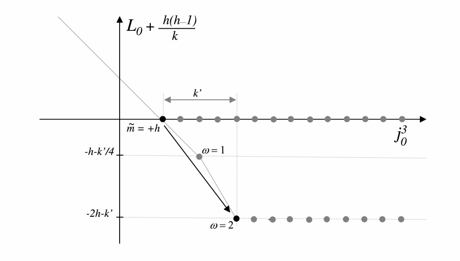
Figure 1: Weight diagram of $SL(2,R)_{k^{\prime}}$. The points in the $j_{0}^{3}$ axis are affine primaries in a $d_{h}^{+}$ representation. The spectral flow of the state with $\tilde{m}=h$ by $w=2$ units gives a state at level $-2h-k^{\prime}$, which is the lowest weight state of a $d_{H}^{+}$ representation of the global algebra with $H=h+k^{\prime}$. All the states of this $d_{H}^{+}$ representation are Virasoro primaries.

We have considered only the holomorphic sector of the theory, but there is a similar anti-holomorphic copy of the currents on which an identical amount of spectral flow must be performed, and the flowed states depend also on indices $\bar{H},\bar{m}$. The operators $\Phi_{m,\bar{m}}^{w}$ that create the flowed modes from the vacuum can be formally summed into the field

$$\Phi_{H,\bar{H}}^{w}(x,\bar{x})=\sum_{m,\bar{m}}\Phi_{m;\bar{m}}^{w}\,x^{-H-m}\bar{x}^{-\bar{H}-\bar{m}}\,,$$ (118)

with

$$H = \tilde{m}+\frac{k^{\prime}}{2}w\qquad\qquad\bar{H}=\tilde{\bar{m}}+\frac{k^{\prime}}{2}w\,.$$ (119)

This field is not an affine primary in the flowed frame $F$, but it is still a Virasoro primary. To see this, note that the positive Virasoro modes in the $F$ frame,

$$L^{H}_{n} = \tilde{L}^{H}_{n}-w\tilde{\jmath}_{n}^{3}\,,$$ (120)

annihilate the state $|\varphi\rangle$, and the operator $j^{+}_{0}$ which creates the other modes commutes with $L_{n}^{H}$. The zero modes of the $SL(2,R)$ currents act on $\Phi_{H,\bar{H}}^{w}(x,\bar{x})$ as

$$j^{A}_{0}\Phi_{H,\bar{H}}^{w}(x,\bar{x})=-D^{A}_{x}\Phi_{H,\bar{H}}^{w}(x,\bar{x})\,,$$ (121)

where $D^{A}_{x}$ are the differential operators (52)-(54) with $h\rightarrow H$, and similarly for the anti-holomorphic sector. Note that we have not mentioned the $SL(2,R)$ spin $h$ of the unflowed representation, since the spin $H$ in the flowed frame $F$ depends only on the value of  $\tilde{m}$. On the other hand, the conformal dimension of $\Phi_{H,\bar{H}}^{w}(x,\bar{x})$ does depend on $h$ and is given, from (109), by

$$\Delta=-\frac{h(h-1)}{k^{\prime}-2}-w\tilde{m}-\frac{k^{\prime}w^{2}}{4}$$ (122)

The expression (118) for $\Phi_{H,\bar{H}}^{w}(x,\bar{x})$ is actually quite schematic. The field should be considered as a meromorphic function of $H,\bar{H}$, and its modes in the $m,\bar{m}$ basis are obtained from the integral transform

$$\Phi_{m,\bar{m}}^{w}=\int\frac{dx^{2}}{|x|^{2}}\,\,x^{H+m}\bar{x}^{\bar{H}+\bar{m}}\Phi_{H,\bar{H}}^{w}(x,\bar{x})\,.$$ (123)

So negative values of $m,\bar{m}$ are obtained also from $\Phi_{H,\bar{H}}^{w}(x,\bar{x})$. Moreover the sign of $w$ is correlated with that of $m,\bar{m}$, so $\Phi_{H,\bar{H}}^{w}(x,\bar{x})$ contains both signs of the spectral flow parameter $w$, and we can use positive $w$ to denote it [27]. A special case occurs when the original state was the lowest weight of a discrete representation $d^{+}_{h}$, with $\tilde{m}=h$. In this case performing spectral flow with $w=-1$ leads to an unflowed lowest weight representation $d^{-}_{\frac{k}{2}-h}$ [25]. Thus, the field in the $x$ basis contains the representations with spectral flow parameters $w$ and $-w-1$. This case will be relevant for us in the flowed chiral operators, and we will denote the operators obtained from $\tilde{m}=\bar{\tilde{m}}=h$, which have $H=\bar{H}=h+k^{\prime}w/2$ by

$$\Phi_{h,w}(x,\bar{x})$$ (124)

instead of $\Phi_{H,\bar{H}}^{w}$.

We refer the reader to [25, 26, 27] for more details on the $SL(2,R)$ spectral flow. We now turn to study how the spectral flow acts in the bosonic $SU(2)_{k^{\prime\prime}}$ sector.

3.2 Spectral Flow in Bosonic $SU(2)$

Let us see how the map of an affine primary into a lowest/highest weight of the global algebra works for the bosonic $SU(2)_{k-2}$ algebra $k^{a}$. If $|\varphi\rangle$ satisfies

$$\tilde{k}^{a}_{s}|\varphi\rangle = 0\,,\qquad\qquad s=1,2,\ldots$$ (125)

$$\tilde{k}^{3}_{0}|\varphi\rangle = \tilde{n}|\varphi\rangle\,,$$ (126)

then, using

$$k_{0}^{\pm} = \tilde{k}_{\mp w}^{\pm}\,,\qquad k_{0}^{3}=\tilde{k}^{3}_{0}-\frac{k^{\prime\prime}}{2}w\,,$$ (127)

we get that in the flowed frame $F$, for $w$ positive,

$$k_{0}^{-}|\varphi\rangle=0\,,\qquad k_{0}^{3}|\varphi\rangle=(\tilde{n}-\frac{k^{\prime\prime}}{2}w)|\varphi\rangle\,\qquad k^{\prime\prime}=k-2\,.$$ (128)

Thus $|\varphi\rangle$ becomes the lowest weight state of a spin $J=-\tilde{n}+\frac{k^{\prime\prime}}{2}w$ representation of the global $SU(2)$. Similarly, for negative $w$, $|\varphi\rangle$ is the highest weight state of a representation with spin $J=\tilde{n}-\frac{k^{\prime\prime}}{2}w$.

As already mentioned, the spectral flow maps the Hilbert space of the $SU(2)$ WZW model to itself. This can be seen from the characters. In the $\tilde{F}$ frame, a spin $j$ character of $SU(2)_{k-2}$ is

$$\mathrm{Tr}(q^{\tilde{L}_{0}-\frac{c}{24}}p^{\tilde{k}^{3}_{0}})=\lambda_{l}(q,p)=\frac{\Theta_{l+1,k}(q,p)-\Theta_{-l-1,k}(q,p)}{\Theta_{1,2}(q,p)-\Theta_{-1,2}(q,p)}\,,$$ (129)

where $l=2j=0,\ldots,k\!-\!2$ and

$$\Theta_{m,k}(q,p)=\sum_{n\in\mathbb{Z}+\frac{m}{2k}}q^{kn^{2}}p^{-kn}\,.$$ (130)

Expressing $L_{0},k^{3}_{0}$ in terms of $\tilde{L}_{0},\tilde{k}_{0}^{3}$, we obtain the corresponding character in the spectral flowed frame $F$ [42],

$$\mathrm{Tr}(q^{L_{0}-\frac{c}{24}}p^{k^{3}_{0}}) = q^{\frac{(k-2)w^{2}}{4}}p^{-\frac{(k-2)w}{2}}\lambda_{l}(q,q^{-w}p)$$ (131)

$$= \left\{\begin{array}[]{ll}\lambda_{l}(q,p)&\quad\textrm{for}\,\,\,\,\,w\in 2\mathbb{Z}\\ \lambda_{k-2-l}(q,p)&\quad\textrm{for}\,\,\,\,\,w\in 2\mathbb{Z}+1\,.\end{array}\right.$$ (134)

So a spin $j$ representation is mapped to a spin $j$ or $\frac{k^{\prime\prime}}{2}-j$ representation, according to whether $w$ is even or odd. A similar mapping of the characters for the $SL(2,R)$ algebra can be found in [43].

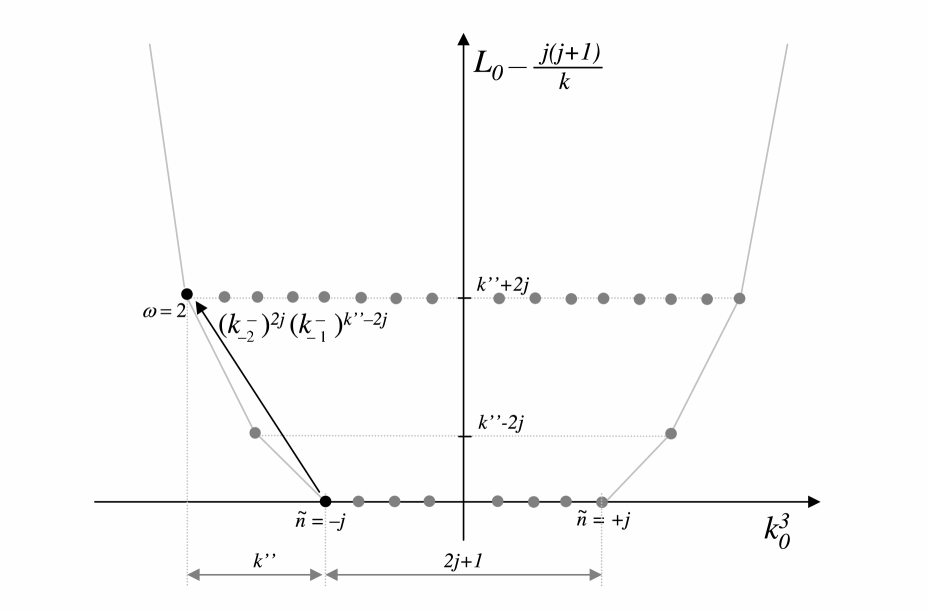
Figure 2: Weight diagram of a spin $j$ representation of affine $SU(2)_{k^{\prime\prime}}$ and the multiplet obtained from spectral flowing the $k_{0}^{3}=-j$ affine primary by $w=2$ units. The points in the $k_{0}^{3}$ axis are $2j\!+\!1$ affine primaries. The affine descendants of the horizontal line at level $k^{\prime\prime}+2j$ are Virasoro primaries which form a representation of the global $SU(2)$ symmetry with spin $J=j+k^{\prime\prime}$.

In the next section, we will be interested in the case when the original unflowed state is an affine primary $|\!-\!j,j\rangle$, with spin $j$, $\tilde{n}=-j$ and $\Delta=j(j+1)/k$. Let us consider $w$ positive. For $w$ even, $w=2p$, we claim that this state is mapped into

$$|\!-\!J,J\rangle\equiv(k^{-}_{-2p})^{2j}(k^{-}_{-2p+1})^{k^{\prime\prime}\!-\!2j}\ldots(k^{-}_{-2})^{2j}(k^{-}_{-1})^{k^{\prime\prime}\!-\!2j}|\!-\!j,j\rangle$$ (135)

with

$$J=j+k^{\prime\prime}p\,.$$ (136)

For $w$ odd, $w=2p+1$, into

$$|\!-\!J,J\rangle\equiv(k^{-}_{-2p-1})^{2j}(k^{-}_{-2p})^{k^{\prime\prime}\!-\!2j}\ldots(k^{-}_{-2})^{k^{\prime\prime}-2j}(k^{-}_{-1})^{2j}|\!-k^{\prime\prime}/2+j,k^{\prime\prime}/2-j\rangle\,,$$ (137)

with

$$J=j+k^{\prime\prime}(p+1/2)\,.$$ (138)

To see that (135) and (137) are the correct states, it is sufficient to note that their quantum numbers are

$$k_{0}^{3} = -j-wk^{\prime\prime}/2\,,$$ (139)

$$L_{0} = \frac{j(j+1)}{k}+jw+\frac{k^{\prime\prime}}{4}w^{2}\,,$$ (140)

as expected from (110) and (111) (with $k\rightarrow k^{\prime\prime}$). For fixed $w$ and $k^{\prime\prime}$, there is a one-to-one correspondence between the quantum numbers $L_{0},k_{0}^{3}$ of the unflowed and the flowed states, hence the multiplicity of the states is preserved under the spectral flow. Since the original state $|\!-\!j,j\rangle$ was the only one with its quantum numbers, this guarantees that  (135) and (137) are the correct states. To verify that the flowed state is a Virasoro primary, note that it lies in the border of the weight diagram of the affine $SU(2)_{k^{\prime\prime}}$ algebra (see Fig. 2), so the action of any Virasoro mode $L_{s}$ with positive $s$ would take it outside of the diagram.

The full multiplet with spin

$$J=j+\frac{k^{\prime\prime}w}{2}$$ (141)

can be generated by acting on (135) and (137) with $k^{+}_{0}$. Let us normalize the states in the multiplet as

$$k_{0}^{3}|n,J\rangle = n|n,J\rangle\,,$$ (142)

$$k^{\pm}_{0}|n,J\rangle = (\pm n+1+J)|n\pm 1,J\rangle\,,$$ (143)

$$k^{\pm}_{0}|\!\pm\!J,J\rangle = 0\,.$$ (144)

Since the $k^{a}_{0}$’s commute with the Virasoro generators, all the members of the multiplet are Virasoro primaries with conformal weight (140). In Figure 2 we ilustrate the position of the elements of this multiplet in the $SU(2)_{k^{\prime\prime}}$ weight diagram for the case $w=2$.

Applying the same amount of spectral flow to the anti-holomorphic sector, the operators $V^{w}_{n,\bar{n}}$, which create the states $|n,\bar{n},J\rangle$ from the vacuum can be summed into

$$V_{j,w}(y,\bar{y}) = \sum_{n,\bar{n}=-J}^{J}V^{w}_{n,\bar{n}}y^{-n+J}\bar{y}^{-\bar{n}+J}\,\,\,.$$ (145)

This field is not an affine primary of the $k^{a}$ currents, but the zero modes act on it as

$$k^{a}_{0}V_{j,w}(y,w)=-P^{a}_{y}V_{j,w}(y,w)$$ (146)

where $P^{a}_{y}$ are the differential operators (64)-(66), with $j\rightarrow J$, and similarly for the anti-holomorphic currents.

In the table below, we summarize the quantum numbers of the $SL(2,R)_{k^{\prime}}$ and $SU(2)_{k^{\prime\prime}}$ states before and after performing spectral flow by $w$ units, with $w>0$.

	$SL(2,R)_{k^{\prime}}$	$SU(2)_{k^{\prime\prime}}$
$\tilde{\jmath}_{0}^{3}$/$\tilde{k}_{0}^{3}$	$\tilde{m}$	$\tilde{n}$
$j_{0}^{3}$/$k_{0}^{3}$	$\tilde{m}+k^{\prime}w/2$	$\tilde{n}-k^{\prime\prime}w/2$
$H/J$	$\tilde{m}+k^{\prime}w/2$	$-\tilde{n}+k^{\prime\prime}w/2$
$\Delta$	$-h(h-1)/(k^{\prime}-2)-w\tilde{m}-k^{\prime}w^{2}/4$	$j(j+1)/(k^{\prime\prime}+2)-w\tilde{n}+k^{\prime\prime}w^{2}/4$

Table 1: Quantum numbers in $SL(2,R)_{k^{\prime}}$ and $SU(2)_{k^{\prime\prime}}$

before and after performing spectral flow by $w>0$ units.

4 Spectral Flow for the Free Fermions

As already mentioned, the spectral flow for the free fermions is just a rearrangement of the spectrum. The effect of this rearrangement is to provide finite dimensional representations of the global $SL(2,R)$ and $SU(2)$ algebras in terms of Virasoro primaries of the $c=\frac{3}{2}$ theories of three fermions. For the $SU(2)$ case, this construction was studied in [44] using an ${\cal N}=1$ theory of a free boson and a free fermion. This is the supersymmetric version of the construction in [45].

For some expressions, it is convenient to have a bosonized form of the fermions. For this, we define

$${\partial}H_{1} = \frac{2}{k}\psi^{2}\psi^{1}\,,$$ (147)

$${\partial}H_{2} = \frac{2}{k}\chi^{2}\chi^{1}\,,$$ (148)

$${\partial}H_{3} = \frac{2}{k}i\psi^{3}\chi^{3}\,.$$ (149)

We normalize the four fermions of $T^{4}$, $\eta^{i},\,i=1\ldots 4$, as

$$\eta^{i}(z)\eta^{j}(w)\sim\frac{\delta^{ij}}{z-w}\,,$$ (150)

and they can be bosonized as

$${\partial}H_{4} = \eta^{2}\eta^{1}\,,$$ (151)

$${\partial}H_{5} = \eta^{4}\eta^{3}\,.$$ (152)

where

$$H_{i}(z)H_{j}(w)\sim-\delta_{ij}\log(z-w)\,.$$ (153)

In order to get the correct anticommutation among the fermions in their bosonized form, we should also introduce proper cocycles [46]. For that, we first define the number operators

$$N_{i}=i\oint{\partial}H_{i}\,,$$ (154)

and then work in terms of bosons redefined as

$$\hat{H}_{i}=H_{i}+\pi\sum_{j<i}N_{j}\,.$$ (155)

The fermions are expressed in terms of $\hat{H}_{i}$ as

$$e^{\pm i\hat{H}_{1}} = \frac{\psi^{1}\pm i\psi^{2}}{\sqrt{k}}\qquad e^{\pm i\hat{H}_{2}}=\frac{\chi^{1}\pm i\chi^{2}}{\sqrt{k}}\qquad e^{\pm i\hat{H}_{3}}=\frac{\chi^{3}\mp\psi^{3}}{\sqrt{k}}\,\,,$$ (156)

and the cocycles pick the right signs using the relation

$$e^{iaN_{j}}e^{ibH_{j}}=e^{ibH_{j}}e^{iaN_{j}}e^{iab}\qquad\qquad j=1\ldots 3\,\,.$$ (157)

In terms of the $\hat{H}_{i}$ bosons, the fermionic currents are

$$\hat{\jmath}^{3} = i{\partial}\hat{H}_{1}\,,$$ (158)

$$\hat{\jmath}^{\pm} = \pm e^{\pm i\hat{H}_{1}}\left(e^{-i\hat{H}_{3}}-e^{+i\hat{H}_{3}}\right)\,,$$ (159)

$$\hat{k}^{3} = i{\partial}\hat{H}_{2}\,,$$ (160)

$$\hat{k}^{\pm} = \mp e^{\pm i\hat{H}_{2}}\left(e^{-i\hat{H}_{3}}+e^{+i\hat{H}_{3}}\right)\,.$$ (161)

4.1 $SL(2,R)$ Fermionic Multiplets

Let us consider the spectral flow in the $\psi^{A}$ sector first. The NS vacuum in the $\tilde{F}$ frame is an excited state in the $T$ frame, given, for positive $w$, by [47]

$$|\tilde{0}\rangle = k^{-w/2}\,\,\psi_{-w+1/2}^{-}\psi_{-w+3/2}^{-}\cdots\psi_{-1/2}^{-}|0\rangle$$ (162)

and for negative $w$

$$|\tilde{0}\rangle = k^{-w/2}\,\,\psi_{-|w|+1/2}^{+}\psi_{-|w|+3/2}^{+}\cdots\psi_{-1/2}^{+}|0\rangle$$ (163)

where the factor $k^{-w/2}$ is to have $\langle\tilde{0}|\tilde{0}\rangle=\langle 0|0\rangle=1$. To check that this representation of $|\tilde{0}\rangle$ in the $F$ frame is correct, note that it is annihilated by $\tilde{\psi}^{\pm}_{n}=\psi^{\pm}_{n\pm w}$ and $\tilde{\psi}^{3}_{n}=\psi^{3}_{n}$ for $n>0$ and that it has $\hat{\jmath}^{3}_{0}=-w$ and $L_{0}=\frac{w^{2}}{2}$, as expected from (98) and (109) with $k=-2$. As we discussed above, for positive $w$, this is the lowest weight state in a representation of $\hat{\jmath}_{0}^{\pm,3}$ with spin $H=\!-w$, which in this case is finite dimensional. So let us call this state

$$|\tilde{0}\rangle=|\!-\!w\rangle\,.$$ (164)

Starting from it we can build the whole multiplet, and we normalize its $2w+1$ states as

$$\hat{\jmath}^{3}_{0}|m\rangle = m|m\rangle$$ (165)

$$\hat{\jmath}^{\pm}_{0}|m\rangle = (m\mp(H-1))|m\pm 1\rangle$$ (166)

$$\hat{\jmath}^{\pm}_{0}|\!\pm\!w\rangle = 0$$ (167)

with $H=-w$. Let us call $U^{w}_{m}$ the fields that create these states from the vacuum. The lowest and highest states have the simple bosonized expression

$$U^{w}_{-w} = e^{-iw\hat{H}_{1}}$$ (168)

$$U^{w}_{w} = e^{iw\hat{H}_{1}}$$ (169)

and since $\hat{\jmath}^{3}=i\partial\hat{H}_{1}$, it is easy to see that they have the correct quantum numbers. We can now formally sum the multiplet into a field $\psi_{w}(x)$,

$$\psi_{w}(x)=\sum_{m=h}^{-h}x^{-H-m}U_{m}^{w}$$ (170)

with $H=-w$. Note that it has fermion number $(-1)^{w}$. For example, for $w=1$ we get

$$\psi_{w=1}(x)\sim-\psi^{+}+2x\psi^{3}-x^{2}\psi^{-}\,,$$ (171)

which is the field called $\psi(x)$ in [7]. From (166) it follows that the zero modes of the currents act on $\psi_{w}(x)$ as

$$\hat{\jmath}^{A}_{0}\psi_{w}(x)=-D_{x}^{A}\psi_{w}(x)$$ (172)

where $D_{x}^{A}$ are the differential operators (52)-(54) with $H=-w$.

One can repeat the same exercise for the three other affine primaries of the $\tilde{F}$ frame in the NS sector, namely, $\tilde{\psi}^{+}_{-1/2}|\tilde{0}\rangle,\tilde{\psi}^{-}_{-1/2}|\tilde{0}\rangle$ and $\tilde{\psi}^{3}_{-1/2}|\tilde{0}\rangle$. We will be interested below in the last two cases.

Consider first the state $\tilde{\psi}^{-}_{-1/2}|\tilde{0}\rangle$ for positive $w$. From (162) and $\tilde{\psi}^{-}_{-1/2}=\psi^{-}_{-w-1/2}$, we have

$$k^{-1/2}\tilde{\psi}^{-}_{-1/2}|\tilde{0}\rangle=k^{-(w+1)/2}\,\,\psi_{-w-1/2}^{-}\psi_{-w+1/2}^{-}\cdots\psi_{-1/2}^{-}|0\rangle$$ (173)

so this state would have come from the $\tilde{F}$ vacuum $|\tilde{0}\rangle$ if we had flowed $w+1$ units instead of $w$. It gives rise to an $SL(2,R)$ multiplet with spin $H=-w-1$, which, summed as in (170), gives the field $\psi_{w+1}(x;z)$.

Consider now, for positive $w$, the state

$$\sqrt{\frac{2}{k}}\tilde{\psi}^{3}_{-1/2}|\tilde{0}\rangle=\sqrt{2}k^{-(w+1)/2}\psi^{3}_{-1/2}\psi_{-1/2}^{-}\psi_{-3/2}^{-}\cdots\psi_{-w+1/2}^{-}|0\rangle$$ (174)

In the $F$ frame, it is the lowest state in a representation of the global $SL(2,R)$ with spin $H=-w$, and conformal dimension $\Delta=\frac{w^{2}}{2}+\frac{1}{2}$. We can now build the whole multiplet as in (166)-(167). Let us call $U^{3,w}_{m}$ to the operators. We can and sum over $x$ as in (170), and we call the corresponding field $\psi_{w}^{3}(x;z)$. Note that it has fermion number $(-1)^{w+1}$. For $w=1$ we get

$$\psi_{w=1}^{3}(x;z)\sim-\hat{\jmath}^{+}(z)+2x\hat{\jmath}^{3}(z)-x^{2}\hat{\jmath}^{-}(z)$$ (175)

which is the field called $\hat{\jmath}(x)$ in [7]. Finally, consider the state

$$\frac{\sqrt{2}}{k}\tilde{\psi}^{3}_{-1/2}\tilde{\psi}^{-}_{-1/2}|\tilde{0}\rangle=\frac{1}{\sqrt{2}}\tilde{\hat{\jmath}}^{-}_{-1}|\tilde{0}\rangle$$ (176)

Following a reasoning similar to the $\tilde{\psi}^{-}_{-1/2}|\tilde{0}\rangle$ case, the corresponding field in the flowed frame $F$ is $\psi_{w+1}^{3}(x;z)$.

4.2 $SU(2)$ Fermionic Multiplets

The case of the $SU(2)$ fermions is similar. The vacuum in the $\tilde{F}$ frame is mapped, for positive $w$, to a state

$$|\tilde{0}\rangle=|\!-\!w\rangle$$ (177)

with $k_{0}^{3}=-w$, which is the lowest weight of a representation of spin $J=w$ for the zero modes $k_{0}^{\pm,3}$ in the flowed frame. We obtain the other states in the multiplet as

$$\hat{k}_{0}^{3}|m\rangle = m|m\rangle\,,$$ (178)

$$\hat{k}_{0}^{\pm}|m\rangle = (J+1\pm m)|m\pm 1\rangle\,,$$ (179)

$$\hat{k}_{0}^{\pm}|\!\pm\!w\rangle = 0\,,$$ (180)

with $J=w$, and the operator that creates the full multiplet is defined as

$$\chi_{w}(y) = \sum_{n=-w}^{w}y^{-n+w}\,T_{n}^{w}$$ (181)

The case $w=1$ is given by

$$\chi_{w=1}(y)\sim-\chi^{+}+2y\chi^{3}+y^{2}\chi^{-}\,,$$ (182)

which is the field called $\chi(y)$ in [7]. The action of the zero modes is now

$$\hat{k}^{a}_{0}\chi_{w}(y;0)|0\rangle=-P_{y}^{a}\chi_{w}(y;0)|0\rangle$$ (183)

where $P_{y}^{a}$ are the differential operators (64)-(66) with $J=w$. The field $\chi_{w}(y,z)$ is a Virasoro primary with dimension $\Delta=\frac{w^{2}}{2}$. Another state which will be useful below is the spectral flow of the state $\tilde{\chi}^{-}_{-1/2}|\tilde{0}\rangle$. By an argument similar as above, in the spectral flowed frame $F$, for $w>0$, it gives rise to the field $\chi_{w+1}(y,z)$.

4.3 The Ramond Sector

The Ramond sector gives fermionic representations with half integer spin, and it is convenient to work with the $SL(2,R)$ and $SU(2)$ together.

We define the Ramond operators in the unflowed frame,

$$\widetilde{S}_{[\epsilon_{1}\,,\epsilon_{2}\,,\epsilon_{3}]}\equiv e^{i\frac{\epsilon_{1}}{2}\widetilde{H}_{1}+i\frac{\epsilon_{2}}{2}\widetilde{H}_{2}+i\frac{\epsilon_{3}}{2}\widetilde{H}_{3}}\,,$$ (184)

and the corresponding states

$$|\epsilon_{1}\,\epsilon_{2}\,\epsilon_{3}\rangle^{\widetilde{}\;}=\widetilde{S}_{[\epsilon_{1}\,,\epsilon_{2}\,,\epsilon_{3}]}|\tilde{0}\rangle\,.$$ (185)

From Table 1, with $k^{\prime}=-2$ and $k^{\prime\prime}=2$, we see that the states $|-\,-\,\pm\rangle^{\widetilde{}}\;$ have $\hat{\jmath}_{0}^{3}=-w-\frac{1}{2}$, $\hat{k}_{0}^{3}=w+\frac{1}{2}$ and $\Delta=\frac{3}{8}+w^{2}+w$. These quantum numbers fix them uniquely (up to an overall phase) to be

$$|-\,-\,\pm\rangle^{\widetilde{}\;} = e^{-i(\frac{1}{2}+w)\hat{H}_{1}-i(\frac{1}{2}+w)\hat{H}_{2}\pm\frac{i}{2}\hat{H}_{3}}|0\rangle$$ (186)

$$= k^{-w}\chi^{-}_{-w}\cdots\chi_{-1}^{-}\,\psi_{-w}^{-}\cdots\psi^{-}_{-1}\,e^{-\frac{i}{2}\hat{H}_{1}-\frac{i}{2}\hat{H}_{2}\pm\frac{i}{2}\hat{H}_{3}}|0\rangle\,.$$ (187)

We will also use the notation

$$|-\,-\,\pm\rangle^{\widetilde{}\;}=|-w/2-1/2\,,-w/2-1/2\,\rangle_{\pm}^{w}\,.$$ (188)

Acting on these states with raising operators $\hat{\jmath}_{0}^{+}$ and $\hat{k}_{0}^{+}$ we find the states $|n_{1}\,,n_{2}\rangle_{\pm}^{w}$, normalized as

$$\hat{\jmath}_{0}^{\pm}|n_{1}\,,n_{2}\rangle_{\kappa}^{w} = (n_{1}\mp(H-1))|n_{1}\pm 1\,,n_{2}\rangle_{\kappa}^{w}\,,\quad H=-w-\frac{1}{2}$$ (189)

$$\hat{\jmath}_{0}^{+}|+(w+\frac{1}{2}),\,n_{2}\rangle_{\kappa}^{w} = 0$$ (190)

$$\hat{k}_{0}^{\pm}|n_{1},\,n_{2}\rangle_{\kappa}^{w} = (J+1\pm n_{2})|n_{1},\,n_{2}\pm 1\rangle_{\kappa}^{w}\,,\quad J=w+\frac{1}{2}$$ (191)

$$\hat{k}_{0}^{\pm}|n_{1},\,\pm(w+\frac{1}{2})\rangle_{\kappa}^{w} = 0\,.$$ (192)

(The above equations hold with the subscript $\kappa$ separately equal to $+$ or $-$). Finally we are in the position to define the states

$$|S^{\pm}_{w}(x,y)\rangle\equiv\sum_{n_{1},n_{2}=-(w+1/2)}^{w+1/2}x^{w/2+1/2-n_{1}}y^{w/2+1/2-n_{2}}\,|n_{1}\,,n_{2}\rangle_{\pm}^{w}\,.$$ (193)

In the table below we summarize the fields that we have defined in the fermionic sectors. They will enter the construction of the 1/2 BPS operators.

Field	$H$	$J$	$\Delta$	Unflowed state	Fermion Number	Sector
$\psi_{w}(x)$	$-w$	-	$\frac{w^{2}}{2}$	$|\tilde{0}\rangle$	$w$
$\psi_{w+1}(x)$	$-w-1$	-	$\frac{(w+1)^{2}}{2}$	$\tilde{\psi}^{-}_{-1/2}|\tilde{0}\rangle$	$w+1$
$\psi_{w}^{3}(x)$	$-w$	-	$\frac{w^{2}}{2}+\frac{1}{2}$	$\tilde{\psi}^{3}_{-1/2}|\tilde{0}\rangle$	$w+1$
$\psi_{w+1}^{3}(x)$	$-w-1$	-	$\frac{(w+1)^{2}}{2}+\frac{1}{2}$	$\tilde{\psi}^{3}_{-1/2}\tilde{\psi}^{-}_{-1/2}|\tilde{0}\rangle$	$w$	NS
$\chi_{w}(y)$	-	$w$	$\frac{w^{2}}{2}$	$|\tilde{0}\rangle$	$w$
$\chi_{w+1}(y)$	-	$w+1$	$\frac{(w+1)^{2}}{2}$	$\tilde{\chi}^{-}_{-1/2}|\tilde{0}\rangle$	$w+1$
$\chi_{w}^{3}(y)$	-	$w$	$\frac{w^{2}}{2}+\frac{1}{2}$	$\tilde{\chi}^{3}_{-1/2}|\tilde{0}\rangle$	$w+1$
$\chi_{w+1}^{3}(y)$	-	$w+1$	$\frac{(w+1)^{2}}{2}+\frac{1}{2}$	$\tilde{\chi}^{3}_{-1/2}\tilde{\chi}^{-}_{-1/2}|\tilde{0}\rangle$	$w$	NS
$S_{w}^{\pm}(x,y)$	$-w-\frac{1}{2}$	$w+\frac{1}{2}$	$\frac{3}{8}+w^{2}+w$	$\tilde{S}^{\pm}(x,y)|\tilde{0}\rangle$		R

Table 2: Fermionic multiplets obtained from $w$ units of spectral flow.

4.4 Interactions of Fermionic Multiplets

The fermionic multiplets we defined are not primaries of the affine algebra. They are however Virasoro primaries, and the zero modes of the $\hat{\jmath}^{A}$ currents act as $D_{x}^{A}$ and $P_{y}^{a}$. This is sufficient to fix the $x$, $y$ and $z$ dependence of their two and three-point functions. Let us consider the NS sector of the $SL(2,R)$ multiplets for concreteness. The two-point functions are

$$\langle\psi_{w}(x_{1};z_{1})\psi_{w}(x_{2};z_{2})\rangle = \frac{(x_{12})^{2w}}{(z_{12})^{w^{2}}}$$ (194)

$$\langle\psi_{w}^{3}(x_{1};z_{1})\psi_{w}^{3}(x_{2};z_{2})\rangle = \frac{(x_{12})^{2w}}{(z_{12})^{w^{2}+1}}$$ (195)

where the coefficient in the rhs is fixed by taking  $x_{1}\rightarrow\infty$ in $x_{1}^{-2w}\psi_{w}(x_{1})$ and $x_{2}=0$, so that eq.(194) becomes

$$\langle V^{w}_{-w}(z_{1})V^{w}_{w}(z_{2})\rangle=\langle e^{-iw\hat{H}_{1}(z_{1})}e^{iw\hat{H}_{1}(z_{2})}\rangle = \frac{1}{(z_{12})^{w^{2}}}$$ (196)

and similarly for eq.(195). The three-point functions of three $\psi$ multiplets are

$$\langle\psi_{w_{1}}(x_{1};z_{1})\psi_{w_{2}}(x_{2};z_{2})\psi_{w_{3}}(x_{3};z_{3})\rangle = f^{(0)}(w_{1},w_{2},w_{3})\,x_{12}^{w_{1}+w_{2}-w_{3}}x_{23}^{w_{2}+w_{3}-w_{1}}x_{31}^{w_{3}+w_{1}-w_{2}}$$ (197)

$$\qquad\times z_{12}^{\Delta_{1}+\Delta_{2}-\Delta_{3}}z_{23}^{\Delta_{2}+\Delta_{3}-\Delta_{1}}z_{31}^{\Delta_{3}+\Delta_{1}-\Delta_{2}}\,,$$

where $\Delta_{i}=w_{i}^{2}/2$. There are actually four possible combinations of $\psi$ and $\psi^{3}$ fields, and we denote their three-point functions as follows

$$\langle\psi_{w_{1}}(x_{1})\psi_{w_{2}}(x_{2})\psi_{w_{3}}(x_{3})\rangle = f^{(0)}(w_{1},w_{2},w_{3})\,,$$ (198)

$$\langle\psi_{w_{1}}(x_{1})\psi_{w_{2}}(x_{2})\psi_{w_{3}}^{3}(x_{3})\rangle = f^{(1)}(w_{1},w_{2};w_{3})\,,$$ (199)

$$\langle\psi_{w_{1}}(x_{1})\psi_{w_{2}}^{3}(x_{2})\psi_{w_{3}}^{3}(x_{3})\rangle = f^{(2)}(w_{1};w_{2},w_{3})\,,$$ (200)

$$\langle\psi_{w_{1}}^{3}(x_{1})\psi_{w_{2}}^{3}(x_{2})\psi_{w_{3}}^{3}(x_{3})\rangle = f^{(3)}(w_{1},w_{2},w_{3})\,.$$ (201)

We have omitted the dependence on the $x_{i}$ and $z_{i}$, which is similar in all the cases. The functions $f^{(0)}$ and $f^{(3)}$ are symmetric in the three arguments, and for $f^{(1)}$ and $f^{(2)}$ we have indicated the symmetries $f^{(1)}(w_{1},w_{2};w_{3})=f^{(1)}(w_{2},w_{1};w_{3})$ and $f^{(2)}(w_{1};w_{2},w_{3})=f^{(2)}(w_{1};w_{3},w_{2})$ by means of the semicolon.

We want to compute now the structure constants $f^{(i)}$. As we mentioned above, the $\psi,\psi^{3}$ multiplets are a generalization to $c=3/2$ of a similar structure that organizes Virasoro primaries of $c=1$ into $SU(2)$ multiplets [45]. For the latter, the three-point functions were computed in [48], and our results below are a generalization of those computations. But instead of computing the four $f^{(i)}$’s, we will see that it is enough to compute $f^{(0)}$ and $f^{(1)}$, and $f^{(2)}$ and $f^{(3)}$ are obtained using supersymmetry.

Consider first $f^{(0)}$. Each field $\psi_{w}(x)$ is a sum over modes $U^{w}_{m}$, given by (170). Taking  $z_{1},x_{1}\rightarrow\infty$ and $z_{2},x_{2}=0$ gives

$$\langle U_{-w_{1}}^{w_{1}}(\infty)U_{w_{2}}^{w_{2}}(0)U^{w_{3}}_{w_{1}-w_{2}}(1)\rangle=f^{(0)}(w_{1},w_{2},w_{3})\,.$$ (202)

First note that if $w_{1}=w_{2}+w_{3}$, the above expression becomes

$$\langle e^{-iw_{1}\hat{H}_{1}(\infty)}e^{iw_{2}\hat{H}_{1}(0)}e^{iw_{3}\hat{H}_{1}(1)}\rangle=1$$ (203)

and similarly for $w_{2}=w_{3}+w_{1}$ and $w_{3}=w_{1}+w_{2}$. When none of these extremal cases occur, we can assume that

$$w_{i}<w_{j}+w_{k}\qquad\qquad i\neq j\neq k\qquad i,j,k=1,2,3\,.$$ (204)

Then we have

$$U^{w_{3}}_{w_{1}-w_{2}}(z) = \frac{1}{p!}(\hat{\jmath}_{0}^{+})^{p}U^{w_{3}}_{-w_{3}}(z)$$ (205)

$$= \frac{1}{p!}\left(\frac{2}{\sqrt{k}}\right)^{p}\!\!\oint\!du_{1}\ldots\oint\!du_{p}\psi^{3}(u_{1})e^{i\hat{H}_{1}(u_{1})}\!\ldots\!\psi^{3}(u_{p})e^{i\hat{H}_{1}(u_{p})}e^{-iw_{3}\hat{H}_{1}(z)}$$ (206)

where

$$p = w_{1}-w_{2}+w_{3}\,\,,$$ (207)

and $p$ should be even so that the total fermion number of the three-point function is even. With the above expression for $U^{w_{3}}_{w_{1}-w_{2}}$, eq.(202) becomes

$$f^{(0)}(w_{1},w_{2},w_{3}) = \frac{1}{p!}\left(\frac{2}{\sqrt{k}}\right)^{p}\!\!\oint\!du_{1}\ldots\oint\!du_{p}\langle\psi^{3}(u_{1})\!\ldots\!\psi^{3}(u_{p})\rangle$$

$$\qquad\qquad\times\prod_{i=1}^{p}u_{i}^{w_{2}}(1-u_{i})^{-w_{3}}\prod_{i<j}(u_{i}-u_{j})$$

The contours of the $u_{i}$’s, which surround the point $z=1$, can be deformed to include the point $z=0$, since the integrand has no singularities at $z=0$. We can then change the exponents infinitesimally into

$$f^{(0)}(w_{1},w_{2},w_{3}) = \frac{1}{p!}\left(\frac{2}{\sqrt{k}}\right)^{p}\!\!\oint\!du_{1}\ldots\oint\!du_{p}\langle\psi^{3}(u_{1})\!\ldots\!\psi^{3}(u_{p})\rangle$$

$$\qquad\qquad\times\prod_{i=1}^{p}u_{i}^{\alpha}(1-u_{i})^{\beta}\prod_{i<j}(u_{i}-u_{j})^{2\rho}$$

where

$$\rho=1/2\qquad\alpha=w_{2}+\epsilon\qquad\beta=-w_{3}-\epsilon$$ (210)

This allows us to further change the contours into the $[0,1]$ segment of the real axis,

$$f^{(0)}(w_{1},w_{2},w_{3})=\left(\frac{\sin(\pi\alpha)}{\pi}\right)^{p}\frac{1}{p!}\left(\frac{2}{\sqrt{k}}\right)^{p}$$ (211)

$$\quad\times\int_{0}^{1}\!\!dt_{1}\ldots\int_{0}^{1}\!\!dt_{p}\langle\psi^{3}(t_{1})\ldots\psi^{3}(t_{p})\rangle\prod_{i<j}(t_{i}-t_{j})^{2\rho}\prod_{i=1}^{p}t_{i}^{\alpha}(1-t_{i})^{\beta}$$

The above integral was computed in [49, 50]. Using eqs. (A.7) and (A.11) in [49] gives

$$f^{(0)}(w_{1},w_{2},w_{3}) = \left(\frac{\sin(\pi\alpha)}{\pi}\right)^{p}\left(\sqrt{2}\right)^{p}\,\prod_{i=0}^{p-1}\frac{\Gamma(1+\alpha+[\frac{i}{2}])\Gamma(1+\beta+[\frac{i}{2}])}{\Gamma(1+\alpha+\beta+\frac{p}{2}+[\frac{i}{2}])}\prod_{i=1}^{p}\frac{\Gamma(i-[\frac{i}{2}])}{\sqrt{2}}\,,$$

which can be expanded as

$$f^{(0)}(w_{1},w_{2},w_{3}) = (\epsilon)^{p}\prod_{i=0}^{p-1}\frac{\Gamma(1+w_{2}+[\frac{i}{2}])\,\Gamma(1-w_{3}-\epsilon+[\frac{i}{2}])\,\Gamma(i+1-[\frac{i}{2}])}{\Gamma(1+w_{2}-w_{3}+\frac{p}{2}+[\frac{i}{2}])}$$ (213)

Using now

$$\Gamma(1-w_{3}-\epsilon+[i/2])\,\Gamma\left(w_{3}+\epsilon-[i/2]\right)\sim\frac{(-1)^{w_{3}-[\frac{i}{2}]}}{\epsilon}$$ (214)

we get, as $\epsilon\rightarrow 0$,

$$f^{(0)}(w_{1},w_{2},w_{3}) = \prod_{i=0}^{p-1}\frac{\Gamma(1+w_{2}+[\frac{i}{2}])\,\Gamma(i+1-[\frac{i}{2}])}{\Gamma(1+w_{2}-w_{3}+\frac{p}{2}+[\frac{i}{2}])\,\Gamma(w_{3}-[\frac{i}{2}])}\,.$$ (215)

Since $p$ is even, this expression can be rearranged into

$$f^{(0)}(w_{1},w_{2},w_{3}) = \prod_{i=1}^{s}\frac{\Gamma^{2}(w_{2}+i)\,\Gamma^{2}(i)}{\Gamma^{2}(\frac{w_{1}+w_{2}-w_{3}}{2}+i)\,\Gamma^{2}(w_{3}+1-i)}$$ (216)

where

$$s = \frac{p}{2}=\frac{w_{1}-w_{2}+w_{3}}{2}\,.$$ (217)

In order to make the symmetry between the $w_{i}$’s in (216) manifest, we can use identities like

$$\prod_{i=1}^{s}\Gamma(w_{2}+i)=\prod_{i=1+w_{2}}^{\frac{w_{1}+w_{2}+w_{3}}{2}}\Gamma(i)=\prod_{i=1}^{w_{2}}\frac{1}{\Gamma(i)}\prod_{i=1}^{\frac{w_{1}+w_{2}+w_{3}}{2}}\Gamma(i)\,,$$ (218)

and all the factors in (216) get expressed in terms of the function

$$R(n)\equiv\prod_{i=1}^{\frac{n}{2}}\Gamma^{2}(i)\,,$$ (219)

defined for $n$ even. This gives finally

$$f^{(0)}(w_{1},w_{2},w_{3})=R\left(w\right)\prod_{i=1}^{3}\frac{R\left(w-2w_{i}\right)}{R(2w_{i})}$$ (220)

where

$$w=w_{1}+w_{2}+w_{3}\,.$$ (221)

Note that the final expression for $f^{(0)}$ is symmetric in the $w_{i}$’s, although this was not manifest in the intermediate steps of the computation.

The computation of $f^{(1)}$ follows along the same lines, the only difference being that now $p$ should be odd in order to have an even total fermion number. The expression for $f^{(1)}$ is given by an integral like (4.4), but with an additional insertion of $\psi^{3}(1)$ in the vev of the $\psi^{3}$ fermions. This integral can be computed using eqs.(A.16)-(A.17) of [49], and leads to

$$f^{(1)}(w_{1},w_{2};w_{3})=\frac{\Gamma\left(\frac{w+1}{2}\right)}{\Gamma(1+w_{3})\Gamma\left(\frac{w_{1}+w_{2}-w_{3}+1}{2}\right)}R\left(w+1\right)\prod_{i=1}^{3}\frac{R\left(w-2w_{i}+1\right)}{R(2w_{i})}$$ (222)

In order to compute $f^{(2)}$ and $f^{(3)}$, we can use that the $\psi^{A}$ fermions have an $N=1$ supersymmetry structure with supercurrent

$$G=\left(\frac{2}{k}\right)^{3/2}\psi^{1}\psi^{2}\psi^{3}=-\left(\frac{2}{k}\right)^{1/2}{\partial}H_{1}\psi^{3}$$ (223)

which relates the multiplets $\psi(x)$ and $\psi^{3}(x)$ as

$$-iw\psi^{3}_{w}(z,x) = \oint dz^{\prime}G(z^{\prime})\psi_{w}(z,x)$$ (224)

$$iw\psi_{w}(z,x) = \oint dz^{\prime}(z^{\prime}-z)G(z^{\prime})\psi^{3}_{w}(z,x)\,.$$ (225)

Expressing $\psi_{w_{1}}(z_{1},x_{1})$ inside the correlation function (197) by means of (225), and changing the contour to encircle $\psi_{w_{2}}(z_{2},x_{2})$ and $\psi_{w_{3}}(z_{3},x_{3})$, one gets

$$w_{1}f^{(0)}(w_{1},w_{2},w_{3}) = w_{2}f^{(2)}(w_{3};w_{1},w_{2})+w_{3}f^{(2)}(w_{2};w_{3},w_{1})\,.$$ (226)

Doing the same operation but starting with $\psi_{w_{2}}(z_{2},x_{2})$ and $\psi_{w_{3}}(z_{3},x_{3})$ gives similarly

$$w_{2}f^{(0)}(w_{1},w_{2},w_{3}) = w_{3}f^{(2)}(w_{1};w_{2},w_{3})+w_{1}f^{(2)}(w_{3};w_{1},w_{2})\,,$$ (227)

$$w_{3}f^{(0)}(w_{1},w_{2},w_{3}) = w_{1}f^{(2)}(w_{2};w_{3},w_{1})+w_{3}f^{(2)}(w_{1};w_{2},w_{3})\,,$$ (228)

and these three equation can be inverted to yield

$$f^{(2)}(w_{1};w_{2},w_{3})=\left(\frac{w_{2}^{2}+w_{3}^{2}-w_{1}^{2}}{2w_{2}w_{3}}\right)f^{(0)}(w_{1},w_{2},w_{3})\,.$$ (229)

One can use similar techniques to express $f^{(3)}$ in terms of $f^{(1)}$. The three-point functions of the $SU(2)$ multiplets $\chi_{w}(y),\chi_{w}^{3}(y)$, are given also by the functions $f^{(i)}$ up to trivial phases.

5 1/2 BPS Flowed Spectrum

The operators ${\cal O}_{h}^{(\epsilon)}(x,y)$ in (72)-(74) have well defined spins, $H=J$, under the total currents $J^{A},K^{A}$, and can be expanded in powers of $x,y$ as

$${\cal O}_{h}^{(-)}(x,y) = e^{-\phi}\sum_{m}\,(\psi\Phi)_{h-1,m}\,x^{-h+1-m}\,\,\sum_{n=-j}^{j}V_{j,n}\,y^{-n+j}$$ (230)

$${\cal O}_{h}^{(+)}(x,y) = e^{-\phi}\sum_{m}\,\Phi_{h,m}\,x^{-h-m}\,\,\sum_{n=-j-1}^{j+1}(\chi V)_{j+1,n}\,y^{-n+j+1}$$ (231)

$${\cal O}_{h}^{(a)}(x,y) = e^{-\frac{\phi}{2}}\,\sum_{m}\sum_{n=-j-1/2}^{j+1/2}(S\Phi V)_{(h-1/2,m+1/2)\atop(j+1/2,n+1/2)}x^{-m-h+1/2}y^{-n+j+1/2}e^{\pm i(\hat{H}_{4}-\hat{H}_{5})}$$ (232)

where in all the cases the relation $j=h-1$ holds, and the two signs of $e^{\pm i(\hat{H}_{4}-\hat{H}_{5})}$ correspond to $a=1,2$. The modes $(\psi\Phi)_{h-1,m},(\chi V)_{j+1,n}$ and $(S\Phi V)_{(h-1/2,m+1/2)\atop(j+1/2,n+1/2)}$ are states in irreducible representations of the tensor product of $\Phi_{h,m}$ and $V_{j,n}$ with the fermions, with the indicated spins and $J^{3}_{0},K^{3}_{0}$ eigenvalues. Their explicit form is

$$(\psi\Phi)_{h-1,m} = -\psi^{+}\Phi_{h,m-1}+2\psi^{3}\Phi_{h,m}-\psi^{-}\Phi_{h,m+1}\,,$$ (233)

$$(\chi V)_{j+1,n} = -\chi^{+}V_{j,n-1}+2\chi^{3}V_{j,n}+\chi^{-}V_{j,n+1}\,,$$ (234)

and

$$(S\Phi V)_{(h-1/2,m+1/2)\atop(j+1/2,n+1/2)}|0\rangle = |++\rangle_{-}\Phi_{h,m}V_{j,n}+\,|+-\rangle_{-}\Phi_{h,m}V_{j,n+1}$$

$$+|-+\rangle_{-}\Phi_{h,m+1}V_{j,n}+|--\rangle_{-}\Phi_{h,m+1}V_{j,n+1}$$

where

$$|\epsilon_{1},\epsilon_{2}\rangle_{-}=(i)^{\frac{1-\epsilon_{2}}{2}}S_{[\epsilon_{1},\epsilon_{2},-\epsilon_{1}\epsilon_{2}]}|0\rangle\,.$$ (236)

and the spin fields $S_{[\epsilon_{1},\epsilon_{2},\epsilon_{3}]}$ are those of (184). The first and second signs in $|\pm\pm\rangle_{-}$ refer to the eigenvalues $\hat{\jmath}_{0}^{3}=\pm 1/2$ and $\hat{k}_{0}^{3}=\pm 1/2$.

We are interested in chiral states whose $SL(2,R)$ part belongs to the spectral flowed representations. It turns out that in order to keep the BRST invariance and the chirality condition $H=J$, the easiest way to proceed is to apply the spectral flow to all the $j^{A},\psi^{A},k^{a},\chi^{a}$ algebras.

1/2 BPS Flowed Spectrum in the NS Sector

Let us start with an ${\cal O}_{h}^{(-)}(x,y)$ operator in the unflowed frame $\tilde{F}$. Since the spectral flow is best defined on states diagonal in $\tilde{J}^{3}_{0}$ and $\tilde{K}^{3}_{0}$, we pick a generic term in its $x,y$ expansion (230). Omitting the $e^{-\phi}$ factor, we consider then the operator

$$(\tilde{\psi}\tilde{\Phi})_{h-1,\tilde{m}}\tilde{V}_{h-1,\tilde{n}}$$ (237)

which, according to (233), creates on the vacuum the state

$$\left(2\tilde{\psi}^{3}_{-1/2}\tilde{\Phi}_{h,\tilde{m}}-\tilde{\psi}^{+}_{-1/2}\tilde{\Phi}_{h,\tilde{m}-1}-\tilde{\psi}^{-}_{-1/2}\tilde{\Phi}_{h,\tilde{m}+1}\right)\tilde{V}_{h-1,\tilde{n}}|\tilde{0}\rangle\,.$$ (238)

Note that we denote the spin in the unflowed frame by $h$. This is a superconformal primary with $\tilde{L}_{0}=1/2$ in the $\tilde{F}$ frame. We consider it now in the physical frame $F$, in which we have performed $w$ units of spectral flow in both $SL(2,R)$ and $SU(2)$, with $w$ positive. The stress tensor and the supercurrent in $T$ are given by [47]

$$L_{s} = \tilde{L}_{s}-w\tilde{J}_{s}^{3}-w\tilde{K}_{s}^{3}\,,$$ (239)

$$G_{r} = \tilde{G}_{r}-w\tilde{\psi}_{r}^{3}-w\tilde{\chi}_{r}^{3}\,.$$ (240)

Note that the terms $\pm\frac{k}{4}w^{2}$ in $L_{0}$ have canceled between $SL(2,R)$ and $SU(2)$. We should require this state to be chiral, have $L_{0}=1/2$ and be annihilated by the positive modes of $L_{s}$ and  $G_{r}$. Imposing $L_{0}=1/2$ we get

$$\tilde{m}=-\tilde{n}\,.$$ (241)

The modes $L_{s>0}$ in (239) clearly annihilate (238). Regarding the supercurrent $G_{r}$ in (240), the modes $\tilde{G}_{r>0}$ and $\tilde{\chi}^{3}_{r>0}$ annihilate (238), but $\tilde{\psi}_{1/2}^{3}$ does not annihilate the first term in (238). Thus we need that term be to absent, which only happens when $\tilde{m}=h-1$, since the $\tilde{\Phi}_{h,\tilde{m}}$ operators belong to a discrete highest weight representation of $SL(2,R)$ in the unflowed frame $\tilde{F}$. We have found then that the state

$$\tilde{\psi}^{-}_{-1/2}\tilde{\Phi}_{h,h}\tilde{V}_{h-1,-(h-1)}|\tilde{0}\rangle$$ (242)

is a superconformal primary with $L_{0}=1/2$ in the $F$ frame. According to our discussion in section 3, it is annihilated by $J^{-}_{0},K^{-}_{0}$, i.e., is the lowest weight of a representation of the global algebra $J^{A}_{0},K^{a}_{0}$ in the flowed $F$ frame, with spins

$$H=J=h-1+\frac{wk}{2}\,,$$ (243)

so the chirality condition is automatically satisfied due to (241). To obtain the rest of the states in the multiplet, we act on (242) with

$$J^{+}_{0}=\hat{\jmath}^{+}_{0}+j_{0}^{+}$$ (244)

$$K^{+}_{0}=\hat{k}_{0}^{+}+k_{0}^{+}$$ (245)

and sum over $x,y$. In the $x,y$ basis the full multiplet will be the product of the operators created by the separate action of $\hat{\jmath}^{+}_{0},j_{0}^{+},\hat{k}_{0}^{+}$ and $k_{0}^{+}$. Note that all the modes in the multiplet will be superconformal primaries with $L_{0}=1/2$, since $J^{+}_{0}$ and $K^{+}_{0}$ commute with $L_{s}$ and $G_{r}$.

We get thus that the type $(-)$ physical chiral operator, in the spectral flowed sector $w$, in the $-1$ picture, is

$${\cal O}_{h,w}^{(-)}(x,y)=e^{-\phi}{\cal O}_{h,w}(x,y)\psi_{w+1}(x)\chi_{w}(y)\,,$$ (246)

where $\psi_{w}(x)$ and $\chi_{w}(y)$ are defined in (170) and (181), and

$${\cal O}_{h,w}(x,y)\equiv\Phi_{h,w}(x)V_{h-1,w}(y)\,,$$ (247)

with $\Phi_{h,w}(x)$ and $V_{h-1,w}(y)$ the holomorphic parts of the operators (124) and (145). The field ${\cal O}_{h,w}(x,y)$ is a kind of spectral flowed version of ${\cal O}_{h}(x,y)$. Its conformal dimension and spins are

$$\Delta = -w^{2}-w\,,$$ (248)

$$H = h+\frac{wk}{2}+w\,,$$ (249)

$$J = h-1+\frac{wk}{2}-w\,.$$ (250)

In the physical operator (246), it appears combined with the field $\psi_{w+1}(x)\chi_{w}(y)$, whose quantum numbers are

$$\Delta = w^{2}+w+\frac{1}{2}\,,$$ (251)

$$H = -w-1\,,$$ (252)

$$J = w\,.$$ (253)

Summing the quantum numbers of the bosonic and fermionic operators gives $\Delta=1/2$ and the chirality relation (243), as expected.

Note that we could also have started by applying, to the original state (238), $w$ units of spectral flow in $SL(2,R)$ and $-w$ units of spectral flow in the $SU(2)$ sector. In the frame $F$, we would get a highest weight state for $SU(2)$, and after summing over the multiplet created by $J^{+}_{0},K^{-}_{0}$ the final operator would coincide with (246).

For the computation of the three-point functions, we will need the form of ${\cal O}_{h,w}^{(-)}(x,y)$ in the zero picture. For this we can apply the picture rasing operator $e^{\phi}G$ to (246). But since $e^{\phi}G$ commutes with $J^{+}_{0},K^{+}_{0}$, it is easier to first change the picture from $-1$ to $0$ in the mode (242) by acting on it with $G_{-1/2}$, expressed as in (240), and only then generate the full multiplet with $J^{+}_{0},K^{+}_{0}$.

We need to use the following commutators

$$\{\tilde{G}_{-1/2},\tilde{\psi}_{-1/2}^{-}\} = \tilde{J}^{-}_{-1}=\tilde{\jmath}^{-}_{-1}+\tilde{\hat{\jmath}}^{-}_{-1}$$ (254)

$$\left[\tilde{G}_{-1/2},\tilde{\Phi}_{h,\tilde{m}}\right] = \frac{2}{k}\tilde{\psi}^{A}_{-1/2}\tilde{\jmath}_{A,0}\tilde{\Phi}_{h,\tilde{m}}$$ (255)

$$\left[\tilde{G}_{-1/2},\tilde{V}_{j,\tilde{n}}\right] = \frac{2}{k}\tilde{\chi}^{a}_{-1/2}\tilde{k}_{a,0}\tilde{V}_{j,\tilde{n}}$$ (256)

and when specializing to $\tilde{m}=h,\tilde{n}=-j$, we also use

$$\tilde{\hat{\jmath}}^{-}_{-1}|\tilde{0}\rangle = \frac{2}{k}\tilde{\psi}^{3}_{-1/2}\tilde{\psi}^{-}_{-1/2}|\tilde{0}\rangle$$ (257)

$$\tilde{\psi}^{-}_{-1/2}\tilde{\psi}^{A}_{-1/2}\tilde{\jmath}_{A,0}\tilde{\Phi}_{h,h}|\tilde{0}\rangle = -h\tilde{\psi}^{-}_{-1/2}\tilde{\psi}^{3}_{-1/2}\tilde{\Phi}_{h,h}|\tilde{0}\rangle$$ (258)

$$\tilde{\chi}^{a}_{-1/2}\tilde{k}_{a,0}\tilde{V}_{j,-j}|\tilde{0}\rangle = -j\tilde{\chi}^{3}_{-1/2}\tilde{V}_{j,-j}|\tilde{0}\rangle+\frac{1}{2}\tilde{\chi}^{-}_{-1/2}\tilde{V}_{j,-j+1}|\tilde{0}\rangle$$ (259)

Collecting all the terms, the picture zero operator in the flowed $F$ frame, expressed in terms of unflowed operators is

$$\left(\tilde{\jmath}_{-1}^{-}+\frac{2}{k}(1-h_{w})\tilde{\psi}^{3}_{-1/2}\tilde{\psi}^{-}_{-1/2}\right)\tilde{\Phi}_{h,h}\tilde{V}_{h-1,-(h-1)}|\tilde{0}\rangle$$ (260)

$$+\frac{2}{k}(1-h_{w})\tilde{\chi}^{3}_{-1/2}\tilde{\psi}^{-}_{-1/2}\tilde{\Phi}_{h,h}\tilde{V}_{h-1,-(h-1)}|\tilde{0}\rangle+\frac{1}{k}\tilde{\chi}^{-}_{-1/2}\tilde{\psi}^{-}_{-1/2}\tilde{\Phi}_{h,h}\tilde{V}_{h-1,-h+2}|\tilde{0}\rangle$$

where

$$h_{w}=h+\frac{kw}{2}$$ (261)

Note that in the last term the unflowed $SU(2)$ primary $\tilde{V}_{h-1,-h}$ has $\tilde{n}=-h$, and not $\tilde{n}=-h-1$ as in the rest of the terms. We can act on this state with $J_{0}^{+},K_{0}^{+}$ and sum over all the states. This gives finally the operator

$${\cal Z}_{h,w}^{(-)}(x,y)={\cal Z}_{h,w}^{(-,1)}(x,y)+{\cal Z}_{h,w}^{(-,2)}(x,y)\,,$$ (262)

where

$${\cal Z}_{h,w}^{(-,1)}(x,y) = \sqrt{1/k}\,j_{-1-w}(x){\cal O}_{h,w}(x,y)\psi_{w}(x)\chi_{w}(y)$$

$$\quad+\sqrt{2/k}(1-h_{w}){\cal O}_{h,w}(x,y)\psi^{3}_{w+1}(x)\chi_{w}(y)\,,$$

$${\cal Z}_{h,w}^{(-,2)}(x,y) = (-1)^{w+1}\sqrt{2/k}(1-h_{w}){\cal O}_{h,w}(x,y)\psi_{w+1}(x)\chi^{3}_{w}(y)$$

$$\quad+(-1)^{w+1}\sqrt{1/k}\Phi_{h,w}(x)V^{\prime}_{h-1,w}(y)\psi_{w+1}(x)\chi_{w+1}(y)\,,$$

These two terms of ${\cal Z}_{h,w}^{(-)}$ come from the first and second line of (260). In the second term of (5), we denoted by $V^{\prime}_{h-1,w}(y)$ the $SU(2)$ multiplet of spin $J=h-2+kw/2$ obtained by spectral flowing the operator $\tilde{V}_{h-1,-h+2}$ (instead of $\tilde{V}_{h-1,-h+1}$). We also defined

$$j_{-1-w}(x)=j_{-1-w}^{+}-2xj_{-1-w}^{3}+x^{2}j_{-\!1\!-w}^{-}$$ (265)

which is a combination of modes of $j^{A}$ with $H=-1$ under the global $SL(2,R)$ algebra.

The reason for splitting ${\cal Z}_{h,w}^{(-)}(x,y)$ into two terms in (262) is that both fermion numbers $F_{\psi}$ and $F_{\chi}$ change by one unit from one term to the other. Since in a non-zero correlator the fermion number should be even independently in the $\psi$ and $\chi$ sectors, whenever ${\cal Z}_{h,w}^{(-,1)}(x,y)$ is non-zero inside a correlator, the contribution of ${\cal Z}_{h,w}^{(-,2)}(x,y)$ will vanish, and viceversa.

Following the same steps for the ${\cal O}_{h}^{(+)}$ operators, leads to the flowed operators

$${\cal O}_{h,w}^{(+)}(x,y)=e^{-\phi}{\cal O}_{h,w}(x,y)\psi_{w}(x)\chi_{w+1}(y)\,,$$ (266)

where now

$$H=J=h_{w}=h+\frac{kw}{2}$$ (267)

In the zero picture this operator becomes

$${\cal Z}_{h,w}^{(+)}(x,y)={\cal Z}_{h,w}^{(+,1)}(x,y)+{\cal Z}_{h,w}^{(+,2)}(x,y)\,,$$ (268)

where

$${\cal Z}_{h,w}^{(+,1)}(x,y) = \sqrt{1/k}\,k_{-1-w}(y){\cal O}_{h,w}(x,y)\psi_{w}(x)\chi_{w}(y)$$

$$\quad+\sqrt{2/k}(1-h_{w}){\cal O}_{h,w}(x,y)\psi_{w}(x)\chi^{3}_{w+1}(y)\,,$$

$${\cal Z}_{h,w}^{(+,2)}(x,y) = (-1)^{w+1}\sqrt{2/k}(1-h_{w}){\cal O}_{h,w}(x,y)\psi^{3}_{w}(x)\chi_{w+1}(y)$$

$$\quad+(-1)^{w+1}\sqrt{1/k}\Phi^{\prime}_{h,w}(x)V_{h-1,w}(y)\psi_{w+1}(x)\chi_{w+1}(y)\,.$$

Here

$$k_{-1-w}(y)=k_{-1-w}^{+}-2yk_{-1-w}^{3}-y^{2}k_{-\!1\!-w}^{-}$$ (271)

is a combination of modes with $J=1$ under the global $SU(2)$ algebra, and $\Phi^{\prime}_{h,w}(x)$ is the field obtained by spectral flowing the operator $\tilde{\Phi}_{h,h+1}$ (instead of $\tilde{\Phi}_{h,h}$ ).

1/2 BPS Flowed Spectrum in the R Sector

To construct the spectral flowed Ramond 1/2 BPS operators in the -1/2 picture, we start from the state

$$\tilde{\phi}_{h,h}\tilde{V}^{w}_{h-1,1-h}\,|-\,-\,-\rangle^{\widetilde{}\;}\,.$$ (272)

It is easy to check that in the $F$ frame, this is a superconformal primary with $L_{0}=\frac{3}{8}$. Moreover, using (240), we see that it is annihilated by $G_{0}$. This ensures that (272) is in the BRST cohomology. Applying the usual procedure of constructing the multiplet in the $(x,y)$ basis, and adding the dependence on the $T^{4}$ twisted fields and on the bosonized ghosts, we arrive at the 1/2 BPS physical operators

$${\cal O}_{h.w}^{(a)}(x,y)=e^{-\phi/2}{\cal O}_{h,w}(x,y)S^{-}_{w}(x,y)\,e^{\pm\frac{i}{2}(\hat{H}_{4}-\hat{H}_{5})}\,.$$ (273)

To obtain the physical operators in the -3/2 picture, it turns out that we need to start with the state

$$\tilde{\phi}_{h,h}\tilde{V}^{w}_{h-1,1-h}\,|-\,-\,+\rangle^{\widetilde{}\;}\,.$$ (274)

This leads to the operators

$${\cal Z}_{h.w}^{(a)}(x,y)=-\frac{\sqrt{k}}{(2h-1+kw)}e^{-3\phi/2}{\cal O}_{h,w}(x,y)S^{+}_{w}(x,y)\,e^{\pm\frac{i}{2}(\hat{H}_{4}-\hat{H}_{5})}\,.$$ (275)

Let us now check that these are the correct expressions for the physical operators in the -3/2 picture. A short computation gives

$$G_{0}\,|{\cal O}_{h,w}(x,y)S^{+}_{w}(x,y)\rangle=-\frac{(2h-1+kw)}{\sqrt{k}}\,|{\cal O}_{h,w}(x,y)S^{-}_{w}(x,y)\rangle\,,$$ (276)

so we see that the operation of picture raising brings us from ${\cal Z}_{h.w}^{(a)}(x,y)$ to ${\cal O}_{h.w}^{(a)}(x,y)$. The relative normalization factor $-(2h-1+kw)/\sqrt{k}$ appearing between the operators in the -1/2 and -3/2 picture will play an important role in the following.

Op.	Pc	Expansion	$F_{\psi}$	$F_{\chi}$	$H\!=\!J$
${\cal O}_{h,w}^{(-)}$	-1	$e^{-\phi}{\cal O}_{h,w}\psi_{w+1}\chi_{w}$	$w\!+\!1$	$w$
${\cal Z}_{h,w}^{(-,1)}$	0	$\sqrt{1/k}j_{-1-w}{\cal O}_{h,w}\psi_{w}\chi_{w}+\sqrt{2/k}(1-h_{w}){\cal O}_{h,w}\psi^{3}_{w+1}\chi_{w}$	$w$	$w$
${\cal Z}_{h,w}^{(-,2)}$	0	$(-1)^{w+1}k^{-\nicefrac{{1}}{{2}}}\psi_{w+1}(\sqrt{2}(1\!-\!h_{w}){\cal O}_{h,w}\chi^{3}_{w}+\Phi_{h,w}V^{\prime}_{h-1,w}\chi_{w+1})$	$w\!+\!1$	$w\!+\!1$	$h_{w}\!-\!1$
${\cal O}_{h,w}^{(+)}$	-1	$e^{-\phi}{\cal O}_{h,w}(x,y)\psi_{w}(x)\chi_{w+1}(y)$	$w$	$w+1$
${\cal Z}_{h,w}^{(+,1)}$	0	$\sqrt{1/k}k_{-1-w}{\cal O}_{h,w}\psi_{w}\chi_{w}+\sqrt{2/k}(1-h_{w}){\cal O}_{h,w}\psi_{w}\chi^{3}_{w+1}$	$w$	$w$
${\cal Z}_{h,w}^{(+,2)}$	0	$k^{-\nicefrac{{1}}{{2}}}\chi_{w+1}(\sqrt{2}(1\!-\!h_{w}){\cal O}_{h,w}\psi^{3}_{w}+\Phi^{\prime}_{h,w}V_{h-1,w}\psi_{w+1})$	$w\!+\!1$	$w\!+\!1$	$h_{w}$
${\cal O}_{h,w}^{(a)}$	$-\frac{1}{2}$	$e^{-\phi/2}{\cal O}_{h,w}(x,y)S^{-}_{w}(x,y)\,e^{\pm\frac{i}{2}(\hat{H}_{4}-\hat{H}_{5})}$
${\cal Z}_{h,w}^{(a)}$	$-\frac{3}{2}$	$-\sqrt{k}(2h_{w}-1)^{-1}e^{-3\phi/2}{\cal O}_{h,w}(x,y)S^{+}_{w}(x,y)\,e^{\pm\frac{i}{2}(\hat{H}_{4}-\hat{H}_{5})}$			$h_{w}\!-\!\frac{1}{2}$

Table 3: Chiral operators in the holomorphic sector with $w$ units of spectral flow.

5.1 The ADE Series

The holographic duality that we are considering assumes the A-series for the modular invariant partition function of the $SU(2)$ WZW model. It is an important open question what the ADE classification of the $SU(2)$ modular invariants [51, 52] corresponds to in the boundary theory. Here we observe that the construction of 1/2 BPS operators can be carried out consistently also in the D and E cases, since the mapping of $SU(2)$ representations under spectral flow (134) is consistent with the ADE classification. Indeed, the level $k^{\prime\prime}$ and the spins $j$ of the representations that appear in the diagonal terms of the D and E modular invariants are ($l=2j$)

$$\begin{array}[]{lll}D_{2t+1}&\qquad k^{\prime\prime}=4t&\qquad l=0,2\ldots k^{\prime\prime}/2\\ D_{2t+2}&\qquad k^{\prime\prime}=4t-2&\qquad l=0,2\ldots k^{\prime\prime}/2\\ E_{6}&\qquad k^{\prime\prime}=10&\qquad l=0,3,4,6,7,10\\ E_{7}&\qquad k^{\prime\prime}=16&\qquad l=0,4,6,8,10,12,16\\ E_{8}&\qquad k^{\prime\prime}=28&\qquad l=0,6,10,12,16,18,22,28\end{array}$$ (282)

We see that whenever a representation $l$ appears, the representation $k^{\prime\prime}-l$ is also present. Therefore, much like in the A case that we have described in detail, each 1/2 BPS operator in the unflowed sector gives rise to infinitely many flowed operators, one for each positive integer $w$.

6 Three-point Functions of 1/2 BPS Flowed Operators

Since all the flowed chiral operators involve the field ${\cal O}_{h,w}=\Phi_{h,w}V_{h-1,w}$, we will be interested in the product of

$$\langle\Phi_{h_{3},w_{3}}(x_{3})\Phi_{h_{2},w_{2}}(x_{2})\Phi_{h_{1},w_{1}}(x_{1})\rangle = \frac{C_{H}(w_{i},h_{i})}{|x_{12}|^{h_{w_{1}}+h_{w_{2}}-h_{w_{3}}}|x_{23}|^{h_{w_{2}}+h_{w_{3}}-h_{w_{1}}}|x_{31}|^{h_{w_{3}}+h_{w_{1}}-h_{w_{2}}}}$$ (283)

and

$$\langle V_{j_{3},w_{3}}(y_{3})V_{j_{2},w_{2}}(y_{2})V_{j_{1},w_{1}}(y_{1})\rangle = C_{S}(w_{i},j_{i})\times|y_{12}|^{j_{w_{1}}+j_{w_{2}}-j_{w_{3}}}|y_{23}|^{j_{w_{2}}+j_{w_{3}}-j_{w_{1}}}|y_{31}|^{j_{w_{3}}+j_{w_{1}}-j_{w_{2}}}$$

with $j_{i}=h_{i}-1$, and we have defined

$$j_{w_{i}}=j_{i}+\frac{k^{\prime\prime}w_{i}}{2}\,.$$ (285)

The dependence of these correlators on $x_{i}$ and $y_{i}$ is fixed by the action of the zero modes (121) and (146). Since the fields $V_{j,w}(y)$ are descendants of $SU(2)$ primaries, their three-point function $C_{S}(w_{i},j_{i})$ can be obtained from those of the primaries using standard techniques. We will not perform these computations in this paper, except for the extremal case $j_{w_{3}}=j_{w_{2}}+j_{w_{1}}$, which is trivial. Still, we can use the $SU(2)$ tensor product rule for the $SU(2)$ spins $j_{w_{i}}$,

$$j_{w_{i}}\leq j_{w_{j}}+j_{w_{k}}\qquad\qquad i\neq j\neq k\qquad i,j,k=1,2,3\,,$$ (286)

and the relation

$$j_{i}\leq j_{j}+j_{k}\,,$$ (287)

which holds between the primaries, to deduce, for (6), the selection rule

$$w_{i}\leq w_{j}+w_{k}\,.$$ (288)

The three-point functions of the $H_{3}^{+}$ model in the unflowed sector were obtained in [53, 54]. General three-point functions in the flowed sectors in the $x$ basis are not known yet, but it was argued in [27] that they satisfy a selection rule less restrictive than (288), given by

$$w_{i}\leq w_{j}+w_{k}+1\,.$$ (289)

As far as we know, the only known flowed three-point function in the $x$ basis was obtained in [61, 27] and corresponds to the case $w_{1}=1,w_{2}=w_{3}=0$. This is allowed by (289), but violates the relation (288) which the chiral operators must obey.

6.1 Fusion Rules

The fusion rules of the boundary correlators are (27)

$$n_{i}\leq n_{j}+n_{k}-1\,,\qquad\qquad i\neq j\neq k\qquad i,j,k=1,2,3\,,$$ (290)

For unflowed representations, these fusion rules coincide in the bulk with those of the WZW model. According to the enlarged bulk-to-boundary dictionary, the lengths $n_{i}$ are

$$n_{i}=2j_{i}+1+kw_{i}$$ (291)

and therefore (290) is equivalent to the fusion rules of the bosonic $SU(2)_{k-2}$,

$$j_{i}\leq j_{j}+j_{k}\,,$$ (292)

combined with the rule (288)

$$w_{i}\leq w_{j}+w_{k}\,.$$ (293)

which we obtained above.

The above results were expressed in the language of $N=4$, but one can verify that the agreement holds also for the $N=2$ fusion rules, including the operators of type $a$.

6.2 String Two-point Functions

In order to compare bulk and boundary three-point functions, operators at both sides should be normalized in the same way. In the chiral operators ${\cal O}_{h,w}^{(\epsilon,{\bar{\epsilon}})}$, both the $V_{j,w}$ and the fermionic factors, as well as the ghosts, have two-point functions normalized to $1$, and the only subtlety comes from the $\Phi_{h,w}$ operator. The two-point functions in the $H_{3}^{+}$ WZW model diverge as

$$\langle\Phi_{h,w}(x_{1})\Phi_{h^{\prime},w}(x_{2})\rangle=|x_{12}|^{-2h_{w}}B(h,w)\delta(h-h^{\prime})\,,$$ (294)

and this divergence comes from the infinite volume of the Killing group in the target space which leaves invariant the positions $x_{1}$ and $x_{2}$ of the two operators. In the string theory two-point functions, this infinite is multiplied by a zero coming from dividing by a similar infinite associated to the Killing group of the worldsheet, thus leading to a finite string theory two-point function [20]. Remarkably, the finite result of this cancelation depends on $h$. Let us call $\Phi_{h,w}(x_{i})S_{i}\,(i=1,2)$ to the full operator, were $S_{i}$ stands for the ghosts, fermions and $SU(2)$ operators. Then the string theory two-point function is

$$\langle\Phi_{h}(x_{1})S_{1}\Phi_{h}(x_{2})S_{2}\rangle_{String}=(2h-1+kw)q_{h}\,|x_{12}|^{-2h_{w}}\,,$$ (295)

where

$$q_{h}=-\frac{1}{2k\pi^{2}}B(h)\,.$$ (296)

Here

$$B(h)=-\frac{\nu^{-2h+1}}{\pi b^{2}}\gamma(1-b^{2}(2h-1))$$ (297)

is the coefficient of the $H_{3}^{+}$ two-point function (294) for the unflowed primaries and we assume

$$\langle S_{1}(1)S_{2}(0)\rangle=1\,.$$ (298)

The expression (295) requires some comments. In the case $w=0$, a detailed derivation of (295) was given in [7] following ideas of [27] (see also [72]). We see that, up to $h$-independent factors, the constant from the cancelation of the infinities is $(2h-1)$.

In the flowed case, one expects changes both in $B(h)$ and in $(2h-1)$. The former should change because the flowed two-point function in the $x$ basis of the $H_{3}^{+}$ WZW model is the two-point function in the $\tilde{m}$ basis of the original operator in the $\tilde{F}$ frame. The explicit form can be found in eq.(5.18) of [27], but when $\tilde{m}=\bar{\tilde{m}}=h$, the contributions depending on $\tilde{m},\bar{\tilde{m}}$ cancel and we get $B(h,w)=B(h)$. As for the $(2h-1)$ factor, it is shown in [27] that it changes to $(2h-1+kw)$ by introducing a suitable regularization of the divergences. We refer the reader to Sec 5.1 of [27] for more details.

Using the above result for the string theory two-point functions, the normalized chiral operators are, in the NSNS sector,

$$\mathbb{O}_{h,w}^{(\epsilon,{\bar{\epsilon}})}(x,y) = \frac{c\,{\cal O}_{h,w}^{(\epsilon,{\bar{\epsilon}})}(x,y)}{\sqrt{q_{h}(2h-1+kw)}}\,,$$ (299)

$$\mathbb{Z}_{h,w}^{(\epsilon,{\bar{\epsilon}})}(x,y) = \frac{c\,{\cal Z}_{h,w}^{(\epsilon,{\bar{\epsilon}})}(x,y)}{\sqrt{q_{h}(2h-1+kw)}}\,,$$ (300)

for $\epsilon,{\bar{\epsilon}}=\pm$. The R sector has an important subtlety. The computation of (295) in the sphere requires the total picture number to be $-2$. So we can take one of the operators in the $-1/2$ picture and the other in the $-3/2$. Taking into account that operators in these two pictures differ by a factor of $(2h-1+kw)^{2}/k$, the string two-point function (295) in the RR sector becomes

$$\langle{\cal O}_{h,w}^{(1,1)}{\cal O}_{h,w}^{(2,2)}\rangle_{String}=\frac{k\,q_{h}}{(2h-1+kw)}\,|x_{12}|^{-2h_{w}}$$ (301)

and therefore the normalized RR operators are

$$\mathbb{O}_{h,w}^{(a,\bar{a})}(x,y) = \sqrt{\frac{(2h-1+kw)}{kq_{h}}}\,c\,{\cal O}_{h,w}^{(a,\bar{a})}(x,y)\,.$$ (302)

The normalized operators in the R-NS cases are similarly obtained. Note that we have included also the $c$ ghost as part of the normalized operators.

6.3 String Three-point Functions

6.3.1 R-R-NS correlators

The two possible correlators of this type are

$$\langle\mathbb{O}^{(2,2)}_{h_{3},w_{3}}(x_{3},y_{3})\mathbb{O}^{(1,1)}_{h_{2},w_{2}}(x_{2},y_{2})\mathbb{O}^{(-,-)}_{h_{1},w_{1}}(x_{1},y_{1})\rangle$$ (303)

$$=\left(\frac{(2h_{w_{3}}-1)(2h_{w_{2}}-1)}{(2h_{w_{1}}-1)q_{h_{1}}q_{h_{2}}q_{h_{3}}}\right)^{\nicefrac{{1}}{{2}}}\frac{g_{6}}{k}\langle{\cal O}^{(2,2)}_{h_{3},w_{3}}(x_{3},y_{3}){\cal O}^{(1,1)}_{h_{2},w_{2}}(x_{2},y_{2}){\cal O}^{(-,-)}_{h_{1},w_{1}}(x_{1},y_{1})\rangle$$ (304)

$$=\left(\frac{(2h_{w_{3}}-1)(2h_{w_{2}}-1)}{(2h_{w_{1}}-1)}\right)^{\nicefrac{{1}}{{2}}}\frac{g_{6}\,C_{H}(w_{i},h_{i})C_{S}(w_{i},j_{i})C^{2}_{f}(w_{i})}{k\sqrt{q_{h_{1}}q_{h_{2}}q_{h_{3}}}}$$ (305)

and

$$\langle\mathbb{O}^{(+,+)}_{h_{3},w_{3}}(x_{3},y_{3})\mathbb{O}^{(1,1)}_{h_{2},w_{2}}(x_{2},y_{2})\mathbb{O}^{(2,2)}_{h_{1},w_{1}}(x_{1},y_{1})\rangle$$ (306)

$$=\left(\frac{(2h_{w_{2}}-1)(2h_{w_{1}}-1)}{(2h_{w_{3}}-1)q_{h_{1}}q_{h_{2}}q_{h_{3}}}\right)^{\nicefrac{{1}}{{2}}}\frac{g_{6}}{k}\langle{\cal O}^{(+,+)}_{h_{3},w_{3}}(x_{3},y_{3}){\cal O}^{(1,1)}_{h_{2},w_{2}}(x_{2},y_{2}){\cal O}^{(2,2)}_{h_{1},w_{1}}(x_{1},y_{1})\rangle$$ (307)

$$=\left(\frac{(2h_{w_{2}}-1)(2h_{w_{1}}-1)}{(2h_{w_{3}}-1)}\right)^{\nicefrac{{1}}{{2}}}\frac{g_{6}\,C_{H}(w_{i},h_{i})C_{S}(w_{i},j_{i})D^{2}_{f}(w_{i})}{k\sqrt{q_{h_{1}}q_{h_{2}}q_{h_{3}}}}$$ (308)

where $j_{i}=h_{1}-1$ and we have omitted the the dependence on $x_{i},y_{i}$, which is standard. The three-point functions $C_{H}(w_{i},h_{i})$ and $C_{S}(w_{i},j_{i})$ were defined in (283) and (6), and $C_{f}$ and $D_{f}$ are

$$C_{f}(w_{i}) = \langle S^{-}_{w_{3}}(x_{3},y_{3})\,S^{-}_{w_{2}}(x_{2},y_{2})\,\psi_{w_{1}+1}(x_{1})\chi_{w_{1}}(y_{1})\rangle\,,$$ (309)

$$D_{f}(w_{i}) = \langle\psi_{w_{3}}(x_{3})\chi_{w_{3}+1}(y_{3})\,S^{-}_{w_{2}}(x_{2},y_{2})\,S^{-}_{w_{1}}(x_{1},y_{1})\rangle\,.$$ (310)

In (305) and (308), these fermionic couplings $C_{f}(w_{i})$ and $D_{f}(w_{i})$ appear squared because we include the holomorphic and antiholomorphic contributions.

For these correlators we will specialize to the $N=2$ extremal three-point functions, which are the cases computed in the boundary theory. The extremality relation is

$$J_{3}=J_{1}+J_{2},$$ (311)

and the correlators (305) and (308) correspond to the $N=2$ cases

$$\begin{array}[]{rclclcr}(\,a\,)&\times&(-)&\rightarrow&(\,a\,)&&\\ (\,a\,)&\times&(\,a\,)&\rightarrow&(+)&&\end{array}$$ (314)

respectively. In the first case (305), the total spin for each operator is

$$J_{1} = j_{1}+kw_{1}/2$$ (315)

$$J_{2} = j_{2}+kw_{2}/2+1/2$$ (316)

$$J_{3} = j_{3}+kw_{3}/2+1/2$$ (317)

and for the second case (308)

$$J_{1} = j_{1}+kw_{1}/2+1/2$$ (318)

$$J_{2} = j_{2}+kw_{2}/2+1/2$$ (319)

$$J_{3} = j_{3}+kw_{3}/2+1$$ (320)

In both cases (311) gives

$$w_{3} = w_{1}+w_{2}\,,$$ (321)

$$j_{3} = j_{1}+j_{2}\,.$$ (322)

and combining these relations with the bulk-to-boundary dictionary

$$n=2j+1+kw$$ (323)

we get

$$n_{3}=n_{1}+n_{2}-1\,,$$ (324)

as in the boundary. In order to get a precise agreement between the bulk structure constants (305) and (308) and the boundary expressions (22) and (23) the following identities should hold

$$\left(\frac{1}{N}\right)^{1/2}=\frac{g_{6}\,C_{H}(w_{i},h_{i})C_{S}(w_{i},j_{i})C^{2}_{f}(w_{i})}{k\sqrt{q_{h_{1}}q_{h_{2}}q_{h_{3}}}}=\frac{g_{6}\,C_{H}(w_{i},h_{i})C_{S}(w_{i},j_{i})D^{2}_{f}(w_{i})}{k\sqrt{q_{h_{1}}q_{h_{2}}q_{h_{3}}}}$$ (325)

We will now turn these expressions into a prediction for $C_{H}(w_{i},h_{i})$, since the other factors can be easily computed. Let us start with the fermionic couplings. The fermionic operators have the expansions

$$\psi_{w}(x) = \sum_{m=-w}^{w}x^{-m+w}\,U_{m}^{w}$$ (326)

$$\chi_{w}(y) = \sum_{n=-w}^{w}y^{-n+w}\,T_{n}^{w}$$ (327)

$$S_{w}^{-}(x,y) = \sum_{m,n=-w-\frac{1}{2}}^{w+\frac{1}{2}}x^{-m+w+\frac{1}{2}}y^{-n+w+\frac{1}{2}}\,S_{m,n}^{(-,w)}$$ (328)

In terms of these modes it is easy to see that

$$C_{f}(w_{i}) = \langle S_{-w_{3}-1/2,-w_{3}-1/2}^{(-,w_{3})}\,\,\,S_{w_{2}-1/2,w_{2}+1/2}^{(-,w_{2})}\,\,\,U^{w_{1}+1}_{w_{1}+1}T^{w_{1}}_{w_{1}}\rangle$$ (329)

$$D_{f}(w_{i}) = \langle U^{w_{3}}_{-w_{3}}T^{w_{3}+1}_{-w_{3}-1}\,\,\,S_{w_{2}-1/2,w_{2}+1/2}^{(-,w_{2})}\,\,\,S_{w_{1}+1/2,w_{1}+1/2}^{(-,w_{1})}\rangle$$ (330)

All the modes are either lowest or highest elements of the multiplet, except for

$$S_{w_{2}-1/2,w_{2}+1/2}^{(-,w_{2})}(0) = \hat{\jmath}_{0}^{-}S_{w_{2}+1/2,w_{2}+1/2}^{(-,w_{2})}(0)$$

$$= \oint_{0}dze^{-i\hat{H}_{1}(z)}\left(e^{+i\hat{H}_{3}(z)}-e^{-i\hat{H}_{3}(z)}\right)e^{i(w_{2}+\frac{1}{2})(H_{1}(0)+H_{2}(0)-\frac{i}{2}H_{3}(0)}\,.$$

Inserting this expression into (329) and (330), we get

$$C_{f}(w_{i})=D_{f}(w_{i}) = \oint_{0}dz(z-1)^{w_{3}}z^{-w_{2}-1}$$ (332)

$$= \frac{w_{1}!w_{2}!}{(w_{1}+w_{2})!}$$ (333)

where we used Cauchy’s theorem in the last line. The result $C_{f}(w_{i})=D_{f}(w_{i})$ is a consistency check on the prediction (325).

Let us consider now $C_{S}(w_{i},j_{i})$. The $k^{3}$ current can be bosonized as

$$k^{3} = i\sqrt{\frac{k^{\prime\prime}}{2}}{\partial}Y\,,$$ (334)

with

$$Y(z)Y(w)\sim-\log(z-w)\,,$$ (335)

and this allows to represent the affine unflowed primaries of $SU(2)_{k^{\prime\prime}}$ as

$$V_{j,\tilde{n}}=e^{i\tilde{n}\sqrt{\frac{2}{k^{\prime\prime}}}Y}\Sigma_{j,\tilde{n}}\,,$$ (336)

where $\Sigma_{j,\tilde{n}}$ are fields in the parafermionic $SU(2)/U(1)$ theory. In this representation, after spectral flow with $w>0$ from the $\tilde{n}=-j$ state, the lowest/highest weight states of the global $SU(2)$ multiplet with spin $j_{w}=j+wk^{\prime\prime}/2$ are

$$V_{\pm j_{w}}^{w}=\left\{\begin{array}[]{ll}e^{\pm ij_{w}\sqrt{\frac{2}{k^{\prime\prime}}}Y}\Sigma_{j,\pm j}&\quad\textrm{for}\,\,w\,\,\textrm{even}\\ e^{\pm ij_{w}\sqrt{\frac{2}{k^{\prime\prime}}}Y}\Sigma_{k^{\prime\prime}/2-j,\,\pm(k^{\prime\prime}/2-j)}&\quad\textrm{for}\,\,w\,\,\textrm{odd}\end{array}\right.$$ (339)

These are the vertex operators that create the states (135) and (137), and their highest weight counterparts. From the extremality condition $w_{3}=w_{2}+w_{1}$, it follows that either all the $w_{i}$’s are even, or two of them are odd. Without loss of generality, we will assume that in the latter case $w_{1}$ and $w_{2}$ are odd. Using the above representation for $V_{\pm j_{w}}^{w}$, we get

$$C_{S}(w_{i},j_{i}) = \langle V_{-j_{w_{3}}}^{w_{3}}V_{j_{w_{2}}}^{w_{2}}V_{j_{w_{1}}}^{w_{1}}\rangle$$ (340)

$$= \left\{\begin{array}[]{ll}\langle\Sigma_{-j_{3},j_{3}}\Sigma_{j_{2},j_{2}}\Sigma_{j_{1},j_{1}}\rangle&\quad\quad\textrm{for all}\,\,w_{i}^{\prime}s\,\,\textrm{even}\\ \langle\Sigma_{-j_{3},j_{3}}\Sigma_{k^{\prime\prime}/2-j_{2},k^{\prime\prime}/2-j_{2}}\Sigma_{k^{\prime\prime}/2-j_{1},k^{\prime\prime}/2-j_{1}}\rangle&\quad\quad\textrm{for}\,\,w_{1},w_{2}\,\,\textrm{odd}\end{array}\right.$$ (343)

$$= \left\{\begin{array}[]{ll}\langle V_{j_{3},-j_{3}}V_{j_{2},j_{2}}V_{j_{1},j_{1}}\rangle&\quad\qquad\textrm{for all}\,\,w_{i}^{\prime}s\,\,\textrm{even}\\ \langle V_{j_{3},-j_{3}}V_{k^{\prime\prime}/2-j_{2},k^{\prime\prime}/2-j_{2}}V_{k^{\prime\prime}/2-j_{1},k^{\prime\prime}/2-j_{1}}\rangle&\quad\qquad\textrm{for}\,\,w_{1},w_{2}\,\,\textrm{odd}\end{array}\right.$$ (346)

These identities follow from the fact that the boson $Y$ is a free field and its contribution to the correlation functions is trivial. In the extremal case $j_{3}=j_{2}+j_{1}$, we have

$$\langle V_{j_{3},-j_{3}}V_{j_{2},j_{2}}V_{j_{1},j_{1}}\rangle=C_{S}(j_{3},j_{2},j_{1})\,.$$ (347)

This is the three-point function of the $SU(2)_{k^{\prime\prime}}$ affine primaries in the $y,\bar{y}$ basis, given by [35]

$$C_{S}(j_{1},j_{2},j_{3})=\sqrt{\gamma(b^{2})}P(j+1)\prod_{i=1}^{3}\frac{P(j-2j_{i})}{P(2j_{i})\sqrt{\gamma((2j_{i}+1)b^{2})}}\,,$$ (348)

where

$$j = j_{1}+j_{2}+j_{3}\,,$$ (349)

$$b = 1/\sqrt{k}\,,$$ (350)

$$\gamma(x) = \frac{\Gamma(x)}{\Gamma(1-x)}\,.$$ (351)

The function $P(s)$ is defined for $s$ a non-negative integer as

$$P(s)=\prod_{n=1}^{s}\gamma(nb^{2})\,,\qquad\qquad P(0)=1\,.$$ (352)

The expression (348) has the remarkable symmetry

$$C_{S}(j_{1},j_{2},j_{3})=C_{S}(j_{1},k^{\prime\prime}/2-j_{2},k^{\prime\prime}/2-j_{3})$$ (353)

and similarly for any pair of $j_{i}$’s, as can be seen from the identity

$$P(s)=P(k-s-1)\,.$$ (354)

Therefore eq.(346) becomes

$$C_{S}(w_{i},j_{i})=C_{S}(j_{i})\,,$$ (355)

for any value of the $w_{i}$’s.

We now have all the elements to go back to (325) and predict the three-point function

$$C_{H}(w_{i},h_{i})=\frac{\sqrt{q_{h_{1}}q_{h_{2}}q_{h_{3}}}}{C_{S}(h_{i}-1)}\left(\frac{(w_{1}+w_{2})!}{w_{1}!w_{2}!}\right)^{2}$$ (356)

for $h_{3}=h_{1}+h_{2}-1$ and $w_{3}=w_{2}+w_{1}$. Note that there was a cancelation between $1/\sqrt{N}$ and $g_{6}/k$, which in particular makes (356) independent of $Q_{1}$, as it should since this is a statement on the worldsheet CFT, which does not depend on $Q_{1}$. The function $C_{S}(j_{i})$ is defined in (348) for semi-integer values of the $j_{i}$’s, but $C_{H}(w_{i},h_{i})$ should be well defined for any values of the $h_{i}$’s. So we expect that the above equation will hold when $C_{S}(j_{i})$ is replaced by its extension to continuous $j_{i}$’s obtained in [7], given by

$$c_{S}(a_{1},a_{2},a_{3})=\frac{\sqrt{\gamma(b^{2})}b^{\frac{1}{2}-b^{2}}}{{\Upsilon}(b)}{\Upsilon}(a+2b)\prod_{i=1}^{3}\frac{{\Upsilon}(a-2a_{i}+b)}{[{\Upsilon}(2a_{i}+b){\Upsilon}(2a_{i}+2b)]^{1/2}}\,,$$ (357)

where $a_{i}=bj_{i}$ and $a=a_{1}+a_{2}+a_{3}$. The function ${\Upsilon}$, introduced in [75], is related to the Barnes double gamma function and can be defined by

$$\log{\Upsilon}(x)=\int_{0}^{\infty}\frac{dt}{t}\left[\left(\frac{Q}{2}-x\right)^{2}e^{-t}-\frac{\sinh^{2}((\frac{Q}{2}-x)\frac{t}{2})}{\sinh\frac{bt}{2}\sinh\frac{t}{2b}}\right]\,.$$ (358)

The integral converges in the strip $0<\textrm{Re}(x)<Q$. Outside this range it is defined by the relations

$${\Upsilon}(x+b)=b^{1-2bx}\gamma(bx){\Upsilon}(x)\qquad{\Upsilon}(x+1/b)=b^{-1+2x/b}\gamma(x/b){\Upsilon}(x)\,.$$ (359)

Using these properties, one can verify that $c_{S}(a_{i})$ reduces to $C_{S}(j_{i})$ for semi-integer $j_{i}$’s.

6.3.2 NS-NS-NS correlators

The type of predictions that we can make in this case are somewhat weaker than in the previous section. For example, let us consider three operators of type $(--)$, such that

$$w_{1}+w_{2}+w_{3}=\,\,\textrm{even}$$ (360)

In order to have total picture $-2$, we consider a string three-point function with two $\mathbb{O}^{(--)}_{h,w}$’s and one $\mathbb{Z}^{(--)}_{h,w}$. Due to the latter, we will need the correlator

$$\langle\Phi_{h_{1},w_{1}}(x_{1})\Phi_{h_{2},w_{2}}(x_{2})j_{-1-w_{3}}(x_{3})\Phi_{h_{3},w_{3}}(x_{3})\rangle = G(h_{i},w_{i})C_{H}(w_{i},h_{i})\,,$$ (361)

where the function $G(h_{i},w_{i})$ carries the effect of the current algebra descendants, and we omitted the $x_{i}$’s and $z_{i}$’s. Unfortunately, since the fields $\Phi_{h_{i},w_{i}}(x_{i})$ are not affine primaries, the standard techniques to obtain $G(h_{i},w_{i})$ cannot be applied. The three-point function we are interested is given then by

$$\langle\mathbb{O}^{(--)}_{h_{1},w_{1}}\mathbb{O}^{(--)}_{h_{2},w_{2}}\mathbb{Z}^{(-,1,-,1)}_{h_{3},w_{3}}\rangle=\frac{g_{6}}{k}\prod_{i=1}^{3}\frac{1}{\sqrt{q_{h_{i}}(2h_{w_{i}}-1)}}$$ (362)

$$\times\,\,C_{H}(h_{i},w_{i})C_{S}(h_{i}-1,w_{i})(f^{(0)}(w_{1},w_{2},w_{3}))^{2}$$

$$\times\,\,\left(f^{(0)}(w_{1}+1,w_{2}+1,w_{3})G(h_{i},w_{i})+\frac{(2-2h_{3})}{\sqrt{2}}f^{(1)}(w_{1}+1,w_{2}+2;w_{3}+1)\right)^{2}$$

where the squares come from the holomorphic and the antiholomorphic contributions, and we omitted the standard dependence on the $x_{i},y_{i}$. The functions $f^{(0)}$ and $f^{(1)}$ come from the fermion interactions and are given by (220) and (222). This expression should coincide with the first line of the boundary correlator (32) with $\epsilon_{i},{\bar{\epsilon}}_{i}=-$, and this implies

$$\,\,C_{H}(h_{i},w_{i})C_{S}(h_{i}-1,w_{i})(f^{(0)}(w_{1},w_{2},w_{3}))^{2}$$

$$\times\,\,\left(f^{(0)}(w_{1}+1,w_{2}+1,w_{3})G(h_{i},w_{i})+\frac{(2-2h_{3})}{\sqrt{2}}f^{(1)}(w_{1}+1,w_{2}+2;w_{3}+1)\right)^{2}$$

$$=(h_{w_{1}}+h_{w_{2}}+h_{w_{3}}-2)^{2}$$ (363)

Similar expressions can be obtained by considering the other cases.

7 Conclusions

We have completed the bulk-to-boundary dictionary for 1/2 BPS operators in $AdS_{3}/CFT_{2}$, giving concrete expressions for the physical bulk vertex operators in the flowed sectors, and we have obtained some partial results about their three-point functions. The structure of the string three-point functions (especially for R-R-NS correlators, where we were able to be more explicit) suggests that the agreement with the boundary results in Sym${}^{N}(T^{4})$ holds in the flowed sectors as well. A definite confirmation of this expectation must await the evaluation of some missing three-point couplings in the $H_{3}^{+}$ WZW model, which is an interesting CFT question in its own right. It would be very interesting to see if the techniques of [53] are effective in this context.

An alternative approach to the evaluation of correlation functions in $AdS_{3}\times S^{3}\times M^{4}$ may be to exploit the ground ring structure discovered in [30]. This approach is very efficient in the minimal string [76] and it would be interesting to see if it can be adapted to this critical background.

References

- [1] J. M. Maldacena, The large n limit of superconformal field theories and supergravity, Adv. Theor. Math. Phys. 2 (1998) 231–252, [hep-th/9711200].
- [2] O. Aharony, S. S. Gubser, J. M. Maldacena, H. Ooguri, and Y. Oz, Large n field theories, string theory and gravity, Phys. Rept. 323 (2000) 183–386, [hep-th/9905111].
- [3] R. Dijkgraaf, On the d1-d5 conformal field theory, Class. Quant. Grav. 17 (2000) 1035–1048.
- [4] J. R. David, G. Mandal, and S. R. Wadia, Microscopic formulation of black holes in string theory, Phys. Rept. 369 (2002) 549–686, [hep-th/0203048].
- [5] E. Martinec, The d1-d5 system, http://hamilton.uchicago.edu/ejm/japan99.ps.
- [6] M. R. Gaberdiel and I. Kirsch, Worldsheet correlators in ads(3)/cft(2), JHEP 04 (2007) 050, [hep-th/0703001].
- [7] A. Dabholkar and A. Pakman, Exact chiral ring of ads(3)/cft(2), hep-th/0703022.
- [8] A. Pakman and A. Sever, Exact n=4 correlators of ads(3)/cft(2), Phys. Lett. B652 (2007) 60–62, [arXiv:0704.3040 [hep-th]].
- [9] A. Jevicki, M. Mihailescu, and S. Ramgoolam, Gravity from cft on s**n(x): Symmetries and interactions, Nucl. Phys. B577 (2000) 47–72, [hep-th/9907144].
- [10] O. Lunin and S. D. Mathur, Correlation functions for m(n)/s(n) orbifolds, Commun. Math. Phys. 219 (2001) 399–442, [hep-th/0006196].
- [11] O. Lunin and S. D. Mathur, Three-point functions for m(n)/s(n) orbifolds with n = 4 supersymmetry, Commun. Math. Phys. 227 (2002) 385–419, [hep-th/0103169].
- [12] M. Mihailescu, Correlation functions for chiral primaries in d = 6 supergravity on ads(3) x s(3), JHEP 02 (2000) 007, [hep-th/9910111].
- [13] G. Arutyunov, A. Pankiewicz, and S. Theisen, Cubic couplings in d = 6 n = 4b supergravity on ads(3) x s(3), Phys. Rev. D63 (2001) 044024, [hep-th/0007061].
- [14] I. Kanitscheider, K. Skenderis, and M. Taylor, Holographic anatomy of fuzzballs, hep-th/0611171.
- [15] M. Taylor, Matching of correlators in , arXiv:0709.1838 [hep-th].
- [16] R. Dijkgraaf, Instanton strings and hyperkaehler geometry, Nucl. Phys. B543 (1999) 545–571, [hep-th/9810210].
- [17] F. Larsen and E. J. Martinec, U(1) charges and moduli in the d1-d5 system, JHEP 06 (1999) 019, [hep-th/9905064].
- [18] J. M. Maldacena and A. Strominger, Ads(3) black holes and a stringy exclusion principle, JHEP 12 (1998) 005, [hep-th/9804085].
- [19] A. Giveon, D. Kutasov, and N. Seiberg, Comments on string theory on ads(3), Adv. Theor. Math. Phys. 2 (1998) 733–780, [hep-th/9806194].
- [20] D. Kutasov and N. Seiberg, More comments on string theory on ads(3), JHEP 04 (1999) 008, [hep-th/9903219].
- [21] J. de Boer, H. Ooguri, H. Robins, and J. Tannenhauser, String theory on ads(3), JHEP 12 (1998) 026, [hep-th/9812046].
- [22] A. Giveon and A. Pakman, More on superstrings in ads(3) x n, JHEP 03 (2003) 056, [hep-th/0302217].
- [23] Y. Hikida, K. Hosomichi, and Y. Sugawara, String theory on ads(3) as discrete light-cone liouville theory, Nucl. Phys. B589 (2000) 134–166, [hep-th/0005065].
- [24] R. Argurio, A. Giveon, and A. Shomer, Superstrings on ads(3) and symmetric products, JHEP 12 (2000) 003, [hep-th/0009242].
- [25] J. M. Maldacena and H. Ooguri, Strings in ads(3) and sl(2,r) wzw model. i, J. Math. Phys. 42 (2001) 2929–2960, [hep-th/0001053].
- [26] J. M. Maldacena, H. Ooguri, and J. Son, Strings in ads(3) and the sl(2,r) wzw model. ii: Euclidean black hole, J. Math. Phys. 42 (2001) 2961–2977, [hep-th/0005183].
- [27] J. M. Maldacena and H. Ooguri, Strings in ads(3) and the sl(2,r) wzw model. iii: Correlation functions, Phys. Rev. D65 (2002) 106006, [hep-th/0111180].
- [28] N. Seiberg and E. Witten, The d1/d5 system and singular cft, JHEP 04 (1999) 017, [hep-th/9903224].
- [29] S. Raju, Counting giant gravitons in , arXiv:0709.1171 [hep-th].
- [30] L. Rastelli and M. Wijnholt, Minimal ads(3), hep-th/0507037.
- [31] E. J. Martinec, G. W. Moore, and N. Seiberg, Boundary operators in 2-d gravity, Phys. Lett. B263 (1991) 190–194.
- [32] C. Vafa and E. Witten, A strong coupling test of s duality, Nucl. Phys. B431 (1994) 3–77, [hep-th/9408074].
- [33] E. D’Hoker, D. Z. Freedman, S. D. Mathur, A. Matusis, and L. Rastelli, Extremal correlators in the ads/cft correspondence, hep-th/9908160.
- [34] J. Fuchs, More on the super wzw theory, Nucl. Phys. B318 (1989) 631.
- [35] A. B. Zamolodchikov and V. A. Fateev, Operator algebra and correlation functions in the two- dimensional wess-zumino su(2) x su(2) chiral model, Sov. J. Nucl. Phys. 43 (1986) 657–664.
- [36] D. Gepner and E. Witten, String theory on group manifolds, Nucl. Phys. B278 (1986) 493.
- [37] D. Kutasov, F. Larsen, and R. G. Leigh, String theory in magnetic monopole backgrounds, Nucl. Phys. B550 (1999) 183–213, [hep-th/9812027].
- [38] D. Friedan, E. J. Martinec, and S. H. Shenker, Conformal invariance, supersymmetry and string theory, Nucl. Phys. B271 (1986) 93.
- [39] B. L. Feigin, A. M. Semikhatov, and I. Y. Tipunin, Equivalence between chain categories of representations of affine sl(2) and n = 2 superconformal algebras, J. Math. Phys. 39 (1998) 3865–3905, [hep-th/9701043].
- [40] J. M. Maldacena, J. Michelson, and A. Strominger, Anti-de sitter fragmentation, JHEP 02 (1999) 011, [hep-th/9812073].
- [41] D. Israel, C. Kounnas, and M. P. Petropoulos, Superstrings on ns5 backgrounds, deformed ads(3) and holography, JHEP 10 (2003) 028, [hep-th/0306053].
- [42] B. L. Feigin, A. M. Semikhatov, V. A. Sirota, and I. Y. Tipunin, Resolutions and characters of irreducible representations of the n = 2 superconformal algebra, Nucl. Phys. B536 (1998) 617–656, [hep-th/9805179].
- [43] A. Pakman, Brst quantization of string theory in ads(3), JHEP 06 (2003) 053, [hep-th/0304230].
- [44] G. Aldazabal, M. Bonini, and J. M. Maldacena, Factorization and discrete states in c = 1 superliouville theory, Int. J. Mod. Phys. A9 (1994) 3969–3988, [hep-th/9209010].
- [45] E. Witten, Ground ring of two-dimensional string theory, Nucl. Phys. B373 (1992) 187–213, [hep-th/9108004].
- [46] V. A. Kostelecky, O. Lechtenfeld, W. Lerche, S. Samuel, and S. Watamura, Conformal techniques, bosonization and tree level string amplitudes, Nucl. Phys. B288 (1987) 173.
- [47] A. Pakman, Unitarity of supersymmetric sl(2,r)/u(1) and no-ghost theorem for fermionic strings in ads(3) x n, JHEP 01 (2003) 077, [hep-th/0301110].
- [48] V. S. Dotsenko, Remarks on the physical states and the chiral algebra of gravity coupled to matter, Theor. Math. Phys. 92 (1992) 938–951, [hep-th/9201077].
- [49] Y. Kitazawa et al., Operator product expansion coefficients in n=1 superconformal theory and slightly relevant perturbation, Nucl. Phys. B306 (1988) 425.
- [50] L. Alvarez-Gaume and P. Zaugg, Structure constants in the n=1 superoperator algebra, Ann. Phys. 215 (1992) 171–230, [hep-th/9109050].
- [51] A. Cappelli, C. Itzykson, and J. B. Zuber, Modular invariant partition functions in two-dimensions, Nucl. Phys. B280 (1987) 445–465.
- [52] A. Cappelli, C. Itzykson, and J. B. Zuber, The ade classification of minimal and a1(1) conformal invariant theories, Commun. Math. Phys. 113 (1987) 1.
- [53] J. Teschner, On structure constants and fusion rules in the sl(2,c)/su(2) wznw model, Nucl. Phys. B546 (1999) 390–422, [hep-th/9712256].
- [54] J. Teschner, Operator product expansion and factorization in the h-3+ wznw model, Nucl. Phys. B571 (2000) 555–582, [hep-th/9906215].
- [55] K. Becker and M. Becker, Interactions in the sl(2,ir) / u(1) black hole background, Nucl. Phys. B418 (1994) 206–230, [hep-th/9310046].
- [56] G. Giribet and C. Nunez, Interacting strings on ads(3), JHEP 11 (1999) 031, [hep-th/9909149].
- [57] N. Ishibashi, K. Okuyama, and Y. Satoh, Path integral approach to string theory on ads(3), Nucl. Phys. B588 (2000) 149–177, [hep-th/0005152].
- [58] K. Hosomichi, K. Okuyama, and Y. Satoh, Free field approach to string theory on ads(3), Nucl. Phys. B598 (2001) 451–466, [hep-th/0009107].
- [59] K. Hosomichi and Y. Satoh, Operator product expansion in string theory on ads(3), Mod. Phys. Lett. A17 (2002) 683–693, [hep-th/0105283].
- [60] Y. Satoh, Three-point functions and operator product expansion in the sl(2) conformal field theory, Nucl. Phys. B629 (2002) 188–208, [hep-th/0109059].
- [61] V. Fateev, A. B. Zamolodchikov, and A. B. Zamolodchikov, unpublished, .
- [62] G. Giribet and C. Nunez, Aspects of the free field description of string theory on ads(3), JHEP 06 (2000) 033, [hep-th/0006070].
- [63] G. Giribet and C. Nunez, Correlators in ads(3) string theory, JHEP 06 (2001) 010, [hep-th/0105200].
- [64] D. M. Hofman and C. A. Nunez, Free field realization of superstring theory on ads(3), JHEP 07 (2004) 019, [hep-th/0404214].
- [65] G. E. Giribet and D. E. Lopez-Fogliani, Remarks on free field realization of sl(2,r)k/u(1) x u(1) wznw model, JHEP 06 (2004) 026, [hep-th/0404231].
- [66] G. Giribet and Y. Nakayama, The stoyanovsky-ribault-teschner map and string scattering amplitudes, Int. J. Mod. Phys. A21 (2006) 4003–4034, [hep-th/0505203].
- [67] S. Ribault, Knizhnik-zamolodchikov equations and spectral flow in ads(3) string theory, JHEP 09 (2005) 045, [hep-th/0507114].
- [68] G. Giribet, On spectral flow symmetry and knizhnik-zamolodchikov equation, Phys. Lett. B628 (2005) 148–156, [hep-th/0508019].
- [69] P. Minces, C. Nunez, and E. Herscovich, Winding strings in ads(3), JHEP 06 (2006) 047, [hep-th/0512196].
- [70] P. Minces and C. Nunez, Four point functions in the sl(2,r) wzw model, Phys. Lett. B647 (2007) 500–508, [hep-th/0701293].
- [71] S. Iguri and C. Nunez, Coulomb integrals for the sl(2,r) wzw model, arXiv:0705.4461 [hep-th].
- [72] O. Aharony, B. Fiol, D. Kutasov, and D. A. Sahakyan, Little string theory and heterotic/type ii duality, Nucl. Phys. B679 (2004) 3–65, [hep-th/0310197].
- [73] P. Christe and R. Flume, The four point correlations of all primary operators of the d = 2 conformally invariant su(2) sigma model with wess- zumino term, Nucl. Phys. B282 (1987) 466.
- [74] V. S. Dotsenko, Solving the su(2) conformal field theory with the wakimoto free field representation, Nucl. Phys. B358 (1991) 547–570.
- [75] A. B. Zamolodchikov and A. B. Zamolodchikov, Structure constants and conformal bootstrap in liouville field theory, Nucl. Phys. B477 (1996) 577–605, [hep-th/9506136].
- [76] I. K. Kostov and V. B. Petkova, Non-rational 2d quantum gravity. i: World sheet cft, hep-th/0512346.