Current address: ]Department of Physics and Astronomy, Dartmouth College, Hanover, NH 03755.
Emergence of Oscillons in an Expanding Background
Abstract
We consider a (1+1) dimensional scalar field theory that supports oscillons, which are localized, oscillatory, stable solutions to nonlinear equations of motion. We study this theory in an expanding background and show that oscillons now lose energy, but at a rate that is exponentially small when the expansion rate is slow. We also show numerically that a universe that starts with (almost) thermal initial conditions will cool to a final state where a significant fraction of the energy of the universe — on the order of 50% — is stored in oscillons. If this phenomenon persists in realistic models, oscillons may have cosmological consequences.
pacs:
11.27.+d 05.70.Ln 98.80.CqI Introduction
A wide range of nonlinear field theories have been found to contain long lived, localized, oscillatory solutions to their equations of motion, known as oscillons or breathers. In the best-known examples DHN ; ColemanQ , conserved charges guarantee the existence of exact periodic solutions. However, in many cases where such arguments are not available, objects with similar properties have also been observed Campbell ; Bogolyubsky ; Gleiser ; 2d ; Honda ; Wojtek ; abelianhiggs ; Forgacs ; Gleiserd ; oscillon ; oscsm ; Gleiserphase ; Gleiserinfl ; Kolb ; GleiserU1 ; hindmarsh .
In this work we consider analytically the evolution of an oscillon in an inflating background. We find that the oscillon is no longer localized and contains a “tail” that slowly leaks energy away. However this decay rate is exponentially suppressed, so we still expect there to exist long-lived objects. This result is in qualitative agreement with numerical work in oscex , which studied the long-term evolution of a single oscillon in an expanding universe background and found that oscillons remain stable for an exponentially long time provided that the horizon is far larger than the width of an oscillon.
Once a model has been shown to contain oscillons, it is natural to ask how easy it is for these coherent objects to form from generic initial conditions. Ref. Gleiserphase showed that oscillons can emerge from a rapid “quench” in which the background potential is suddenly changed, throwing the system far out of equilibrium. Here we consider the opposite situation: We begin with an (almost) thermal distribution at high temperature and gradually cool the system by coupling it to an expanding background. This setup is suggestive of a situation that could arise in the early universe, for example as the universe cools after reheating or a phase transition. If stable oscillons formed in these situations, they might have cosmological consequences: e.g., see Gleiserinfl . Although it did not consider oscillons, Rajantie found significant non-thermal effects in electroweak baryon number violating processes. Ref. riotto studied a case similar to ours, but involving a different type of oscillon that is stable only if its amplitude exceeds a certain critical value. This situation is quite different from our model, in which there is no such threshold amplitude.
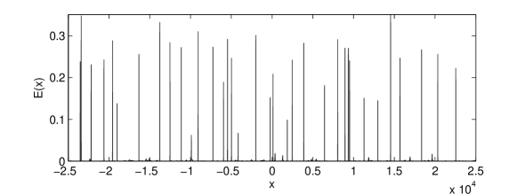
For numerical convenience, we work with a single scalar field in one dimension, though we have seen qualitatively similar results in simulations of the two-dimensional scalar model of 2d in an expanding background. We start at a temperature for which the universe is dominated by radiation and allow the universe to expand until it contains only a cold, pressureless dust of both oscillons and fundamental excitations of the field. A late-time snapshot of the energy density of such a configuration as a function of position is shown in Figure 1, where the sharp spikes are oscillons. We find that a sizeable fraction of the energy of this final state — of order 50% or more — is stored in oscillons. This result persists even for very small coupling constants, where quantum effects are small and do not affect our classical field theory analysis.
II Model
We consider a toy model consisting of a massive scalar field in a one-dimensional expanding background. In terms of the comoving coordinate , the model is described by the Lagrangian
| (1) |
where an overdot denotes a derivative with respect to and a prime denotes a derivative with respect to . Note that this potential has a unique minimum at , with no other extrema or inflection points. It does not support static solitons, but does support oscillons. This Lagrangian leads to the equation of motion
| (2) |
For simplicity we take the expansion rate to be constant. Although we hope that our model can shed light on the reheating phase of inflation, during which would be rapidly decreasing, for our purposes it is only important that the expansion rate be slow compared to the typical time scales of the oscillon.
All known oscillon solutions have been found for massive fields, with frequency of oscillation below the threshold for fundamental excitations, so we have chosen a massive field. The sign of the term, the leading nonlinearity, is crucial: it has been chosen so that to leading order this term decreases the frequency of small oscillations. With the other sign we do not see any oscillons form. Finally, the term exists to eliminate instabilities at large field values introduced by the choice of sign of the term. Because the oscillons involve only moderate excitations of the field, this term does not play an important role in their dynamics.
We have scaled the self-interaction terms by a small parameter . The exact meaning of this parameter is somewhat subtle, since by defining a new field variable we can shift completely outside the Lagrangian (1), which means that it no longer appears in the classical equations of motion. The full quantum theory is still sensitive to the value of , but only in the combination ; therefore a classical approximation involving small is equivalent to one involving small , and the results of our classical analysis are valid provided that is small.111Also, throughout this paper the quantity we call has dimensions of [length]-1, not energy, and is thus really the mass of a single elementary quantum divided by .
III Small-amplitude analysis of oscillons
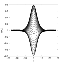
To describe the oscillons we expect to emerge from the thermal background in our simulation, we use a small-amplitude analysis, following smallamp . In particular (e.g. see oscex ) in a static background the equation of motion (2) supports solutions that are localized in space and periodic in time. These oscillons can be expanded in a small parameter . The amplitude of the oscillations scales with , the spatial width of the oscillon is proportional to , and the oscillation frequency is given by . Numerical calculations indicate that there is an upper bound on how large can be for a stable solution: , where .
Here we extend these results to an inflationary background. A sufficiently fast expansion will result in a horizon that is comparable to the minimum oscillon width (proportional to ), preventing oscillons from ever forming. If the expansion rate is slow, long lived oscillons can occur in the range , as shown below. In this regime the oscillon radiates energy away (in the form of scalar field waves) at a rate that is exponentially small in the dimensionless ratio . If this ratio becomes sufficiently large, numerical calculations show that the oscillon is not affected by the expansion in any way that we can detect.
III.1 Separation of scales
We work in static patch coordinates on de Sitter space (e.g., see desitter ) where the metric takes the form
| (3) |
These coordinates are valid for . In these coordinates the equation of motion (2) becomes
| (4) |
Here an overdot indicates a derivative with respect to and a prime indicates a derivative with respect to . Now we follow oscex and change to variables and , where is the small parameter mentioned above. Note that since the horizon distance is and the oscillon width is , to obtain a stable oscillon solution we expect . We therefore let , where is taken to be a small dimensionless number. The power of in this expression is important: If instead we take to be then no oscillon solution is possible, while if we take to be then (to the order we are working) the oscillon does not feel the expansion.
In terms of and the equation of motion is
| (5) |
We expand in powers222Note that the expansion (6) involves only odd powers of . This is consistent with (5) because this equation is odd in , and depends on via only. of as
| (6) |
and seek oscillons, solutions that are periodic (with period ) in and localized in space. In fact, as we will show below, these solutions are neither strictly periodic nor localized, but these departures are exponentially small and occur over time scales much longer than the one given by .
We now substitute (6) into the governing equation (5) and solve it order by order in . At ,
| (7) |
Thus , where the profile remains to be determined. We can find this profile by considering the equation
| (8) |
The key point here is that the only way that can be periodic in is if the forcing terms on the right-hand side of the equation are orthogonal to , since otherwise would have a component that grows linearly in . Therefore we set the Fourier coefficients of to , and obtain a self-contained ordinary differential equation for the oscillon profile:
| (9) |
For a “perfect” oscillon, a localized (exponentially decaying as ) spatial profile is needed. This, however, is not quite possible. The behavior of the above equation changes at : for small the equation is essentially the same as the equation for a flat-space oscillon, while for large the term dominates, giving oscillatory behavior that causes the oscillon to radiate (a small amount of) energy away. Note that this change in behavior occurs well before the horizon, which is at .
III.2 Asymptotic Behavior
First we examine the regime where . Here the term arising from the expansion of the universe is negligible and the equation reduces to the case of a static background. Therefore, we can take
| (10) |
Note that since , the oscillon behaves like in the region . In particular, while its amplitude does not quite vanish (since we cannot take in the equation above), it fails to be fully localized only because of an exponentially small tail, as is shown below.
We now relax the upper bound and consider the region where (an entirely similar calculation can be done where ). From the reasoning above, we see that on the left-hand side of this region, the field is exponentially small. Thus, provided that the field does not grow too much as increases in this region, we are justified in neglecting the nonlinear term in the equation, though we must now take into account the effects of the expansion. Thus we obtain
| (11) |
This equation can be put into a more familiar form by defining a new coordinate . Then we obtain
| (12) |
This is exactly the Schrödinger equation for the wave function of a particle in an upside-down harmonic oscillator with energy , with the dimensionless Hubble constant playing the same role as Planck’s constant in the analogous quantum mechanics problem. At small the particle is in the “classically forbidden” region of the potential and the wavefunction is exponentially suppressed, corresponding to the exponential tail of the oscillon. For any nonzero value of , we eventually enter a “classically allowed” region and the wavefunction becomes oscillatory, which for our classical field profile indicates an outgoing wave that carries energy away. Therefore this situation looks exactly like a quantum mechanics tunneling problem, and since we are interested in small we can use a semiclassical approximation to solve it.333Of course, exact formal solutions for the wavefunction of an upside-down oscillator exist in terms of Hermite functions. However, extracting the asymptotic behavior from these special functions is somewhat messy; for our purposes we can obtain equivalent results simply using WKB.
Choosing an outgoing wave boundary condition as , the standard WKB connection formulae gottfried give us the following relation between the wavefunctions on either end of the turning point at :
where the left-hand side is valid for , the right-hand side is valid for , and is an overall constant.
Performing the integrals, keeping only the leading dependence, and replacing with , we obtain
| (13) | ||||
| (14) |
As expected, the small behavior of (13) is of exactly the correct form to fit the large asymptotic behavior of (10). Matching to this result sets to and hence fixes the coefficient of the outgoing wave (14).
Returning to our original variables and putting together the pieces, we find the following expressions for the oscillon
| (15) | ||||
| (16) |
From here it is easy to compute the relevant components of the stress tensor and find the rate of energy flux. If we take the energy stored in a region to be , then using the conservation of the stress tensor and (16) we obtain
| (17) |
where the region is taken to be a symmetric interval and is far enough from the origin that (16) holds. Note that to leading order all dependence comes from the curvature of the metric; if we restrict attention to (i.e. we consider only a small neighborhood of the oscillon) then space looks almost flat and we obtain
| (18) |
This is our main result. While an oscillon can live forever on a flat background (at least as a formal perturbation series), this is no longer the case in a de Sitter universe; instead it is forced to radiate energy away, albeit through a mode that is exponentially suppressed.
IV Thermal initial conditions
We would like to start our simulations using initial conditions mimicking those of the interacting field theory defined by the Lagrangian (1) at nonzero temperature . However, constructing this equilibrium is quite difficult; although we are essentially interested in classical physics, a classical treatment of this field theory at nonzero temperature suffers from the Jeans paradox. In a quantum treatment we avoid this problem, but we are still unable to systematically take into account the nonlinear terms in the Lagrangian: as is shown below, we will be interested in temperatures , which is precisely the regime where finite temperature perturbation theory fails.
We shall thus take a different approach and generate our initial conditions to simulate thermal states of the free massive scalar field. We note that for the reasons stated above these quasi-thermal initial conditions are probably quite far from the true thermal equilibrium of the full interacting theory; hence the parameters and should be thought of more as measures of the amplitude and width of our distribution in momentum space than as directly physically relevant quantities. We show, however that provided is sufficiently high, all other numerically feasible variations of these parameters produce oscillons in copious numbers, leading us to believe that our results are independent of any particular details of the initial conditions.
To construct these conditions, we return to comoving coordinates. Since our real interest is in a numerical simulation we impose both infrared and ultraviolet cutoffs, placing the system in a box of comoving size and on a regular lattice with spacing . We replace the spatial derivatives by finite differences (see the Numerical Simulation section) and label the free field’s normal modes by , where and is the number of lattice points. Finally we take the scale factor at this time to be .
On this lattice each free mode is described by a harmonic oscillator with frequency
| (19) |
The initial conditions for are then given by
| (20) | |||||
| (21) |
where is a random complex variable with phase distributed uniformly on and magnitude drawn from a Gaussian distribution such that
| (22) |
This is the usual amplitude distribution for a quantum harmonic oscillator LL with the zero-point motion subtracted. On average, these initial conditions assign energy to modes with , in agreement with equipartition. The energy per mode goes rapidly to zero for , giving a total energy density that scales like for , as usual for blackbody radiation in one dimension. Oscillons will form from the energy density in modes with wavelengths of order , which scales like . For oscillons to form, this energy density must be at least of order , so that the fields will have amplitude and the nonlinear interaction terms can balance the dispersive gradient terms. Therefore we will need an initial temperature of to form oscillons.
We have simply subtracted off the zero-point quantum fluctuations in the field. Although it is well-known that these fluctuations have significant consequences for the evolution of a classical field in an expanding background Guth:1985ya , these effects are most important at very long length scales, of order . For small , the oscillon solution comprises many fundamental excitations of the field at the length scales of order that are relevant to oscillon formation and stability. Thus the quantum effects we are neglecting should not change our results significantly. Alternatively, this quantum prescription can simply be thought of as describing a classical equilibrium with short-distance cutoff . (A method to eliminate such cutoff dependence of classical simulations is discussed in Borrill:1996uq ).
As the universe expands, it cools and loses energy according to
| (23) |
where the pressure density is
| (24) |
In equilibrium at temperatures much greater than , if we neglect the interaction terms, the system looks like massless radiation, with pressure density approximately equal to its energy density. In equilibrium at low temperatures, the field is slowly varying in space, with only small values of excited, and of small amplitude. In that case the gradient and nonlinear terms are negligible and , so the pressure goes to zero and the system behaves like pressureless dust.
V Numerical Simulation
We discretize at the level of the Lagrangian in Eq. (1), working in natural units where . For the space derivatives we use ordinary first-order differences,
| (25) |
where refers to the value of at lattice point . We work on a regular lattice with spacing and impose periodic boundary conditions. Varying this Lagrangian yields lattice equations of motion with second-order space derivatives,
| (26) |
We then express this second order equation as a set of coupled first order differential equations and step forward in time using a standard fourth-order Runge-Kutta integrator (e.g., see numrec ). The Courant condition requires that we maintain for numeric stability. Of course this allows us the possibility of rescaling as the simulation runs; this rescaling stops when we reach a maximum value of .
As the universe expands, the oscillons maintain a fixed size in physical units. On the other hand, our lattice expands with the universe. Thus we add new lattice points whenever the lattice spacing exceeds some fixed size in physical units. This is accomplished by refining the lattice, doubling the total number of lattice points and bringing the lattice spacing back to in physical units. We assign values to the field for the new intermediate lattice points by linear interpolation.
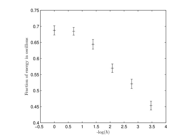
We performed several checks on our numerics. We would like to take sufficiently small that given a set of initial data any further reduction of does not significantly change the final configuration after a run. In the strongly nonlinear regime in which we work, this turns out to be a technically very difficult goal to achieve, with different timesteps often resulting in significantly different final configurations. In fact, despite our best efforts the upper end of Fig. 3, where , suffers from this problem, so we cannot guarantee the validity of this region of the plot, although the remainder of the plots we present satisfy all of our tests. We also verify that all of our simulations maintain energy conservation (as given by Eq. (23)) to better than one part in , and that is small enough that further reduction does not significantly alter the final configuration obtained after a run.
VI Results
We simulate the scalar field in an expanding universe varying the initial temperature and the value of (which determines the effective coupling ). We are interested in determining what fraction of energy in the universe ends up in oscillons; we estimate this as the integral of the energy density over regions of space at which the energy density is more than five times the average energy density, divided by the total energy. As shown in Fig. 1, oscillons stand so much higher than the background fluctuations that this is a good measure. For each run we expand until this quantity reaches a constant value, indicating that the system has stabilized. We then plot this quantity as a function of the parameters in the initial conditions in Fig. 2 and Fig. 3.
Fig. 1 shows a snapshot of the energy density as a function of position for a typical run. We see that the oscillons are very clearly defined, with energy densities far above the background from ordinary field fluctuations. At these late times, the ordinary fluctuations are of small amplitude, and have been redshifted to large spatial wavelengths; they have and . From Eq. (24), we see that the pressure of such fluctuations vanishes: the and terms cancel, and the gradient and nonlinear terms can be neglected because the ordinary fluctuations are slowly varying in space and have small amplitude. So the total energy in ordinary fluctuations remains constant, corresponding to a pressureless dust of ordinary particles of mass at rest. As the universe continues to expand, the energy density in these fluctuations decreases, since it scales inversely with the volume of the universe to keep the total constant. The oscillons, meanwhile, maintain fixed physical size, energy density, and total energy — and therefore zero pressure — but are brought to rest relative to the expanding background. As a result, they also appear as a pressureless dust at late times.
In Fig. 2 we vary in the initial conditions and examine the variation of the fraction of energy in the universe in oscillons. Each point on the graph is an average over many runs, with error bars indicating the standard deviation. (Because our initial conditions are random individual representatives drawn from the initial thermal distribution, our results can vary from one run to the next.) As we move to the right on the logarithmic scale on the horizontal axis, becomes smaller and the quantum effects we have neglected are less important. We see that the fraction of energy in oscillons remains substantial, decreasing only gradually as decreases to small values.
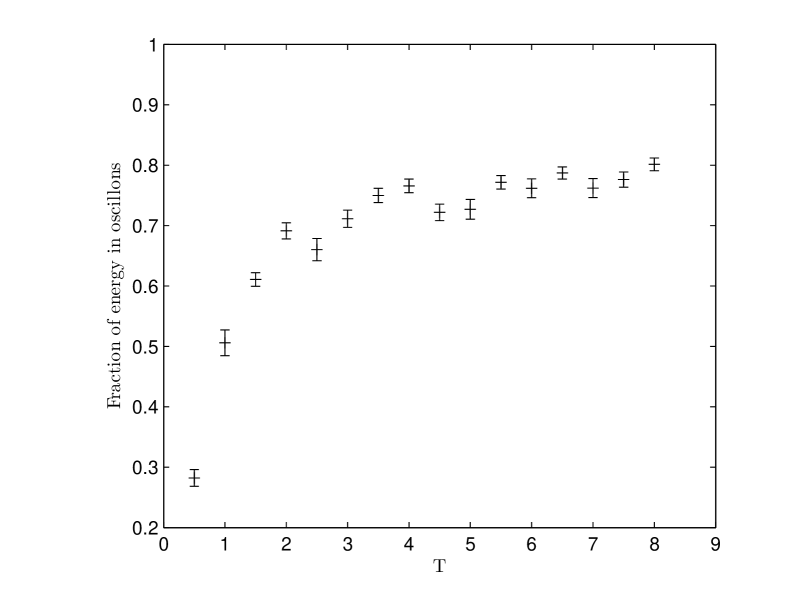
Fig. 3 shows the fraction of energy in oscillons for a range of initial temperatures. For large enough, we see that the result saturates, so that higher initial temperatures no longer affect the final result. In the saturated regime, the system is just undergoing ordinary cooling, remaining at equilibrium as the temperature begins to decrease. It is only once the system cools below that the oscillons begin to emerge. So while we are always imagining our system starts out at very high temperatures compared to the energy scales relevant to oscillon formation, in practice we only need to start our simulations at temperatures just above the saturation point.
VII Discussion and Conclusions
We have considered a scalar field theory that supports stable oscillons. We place this theory in an expanding background and show that the oscillons are no longer completely stable but instead lose energy at a rate that is exponentially small in the size of the horizon. We also find numerically that quasi-thermal initial conditions result in the eventual formation of oscillons in large numbers. Though the oscillons are large, coherent objects, they nevertheless form easily from a random superposition of momentum modes, suggesting that in some sense they are attractors in the solution space of the equations of motion. In our model they capture a significant portion of the energy of the universe, on the order of 50%. Though this paper deals with a one-dimensional case, we have seen qualitatively similar results in two dimensions. If this phenomenon persists in realistic models (and in a realistic number of dimensions), oscillons may have cosmological consequences, as discussed in Ref. Gleiserinfl .
VIII Acknowledgments
We thank N. Alidoust, A. Scardicchio, and R. Stowell for assistance and M. Gleiser for helpful discussions. E. F. and A. H. G. were supported in part by funds provided by the U. S. Department of Energy (D. O. E.) under cooperative research agreement DE-FC02-94ER40818. N. G. and N. S. were supported by National Science Foundation (NSF) grant PHY-0555338, by a Cottrell College Science Award from Research Corporation, and by Middlebury College. N. I. was supported in part by National Science Foundation (NSF) Graduate Fellowship 2006036498.
References
- (1) R. F. Dashen, B. Hasslacher, and A. Neveu, Phys. Rev. D11 (1975) 3424.
- (2) S. Coleman, Nucl. Phys. B262 (1985) 263.
- (3) D. K. Campbell, J. F. Schonfeld and C. A. Wingate, Physica 9D, 1 (1983).
- (4) I. L. Bogolyubsky and V. G. Makhankov, JETP Lett 24 (1976) 12.
- (5) M. Gleiser, hep-ph/9308279, Phys. Rev. D49 (1994) 2978; E. J. Copeland, M. Gleiser and H. R. Muller, hep-ph/9503217, Phys. Rev. D52 (1995) 1920; A. B. Adib, M. Gleiser, and C. A. S. Almeida, hep-th/0203072, Phys. Rev. D66 (2002) 085011; G. Fodor, P. Forgács, P. Grandclément and I. Rácz, hep-th/0609023, Phys. Rev. D74 (2006) 124003.
- (6) M. Gleiser and A. Sornborger, patt-sol/9909002, Phys. Rev. E62 (2000) 1368; M. Hindmarsh and P. Salmi, hep-th/0606016, Phys. Rev. D74 (2006) 105005.
- (7) E. P. Honda and M. W. Choptuik, hep-ph/0110065, Phys. Rev. D65 (2002) 084037.
- (8) B. Piette and W. J. Zakrzewski, Nonlinearity 11 (1998) 1103.
- (9) C. Rebbi and R. J. Singleton, hep-ph/9601260, Phys. Rev. D54 (1996) 1020; P. Arnold and L. McLerran, Phys. Rev. D37 (1988) 1020;
- (10) G. Fodor and I. Racz, hep-th/0311061, Phys. Rev. Lett. 92 (2004) 151801; P. Forgacs and M. S. Volkov, hep-th/0311062, Phys. Rev. Lett. 92 (2004) 151802.
- (11) M. Gleiser, hep-th/0408221, Phys. Lett. B600 (2004) 126; P. M. Saffin and A. Tranberg, hep-th/0610191.
- (12) E. Farhi, N. Graham, V. Khemani, R. Markov, and R. R. Rosales, hep-th/0505273, Phys. Rev. D72 (2005) 101701(R).
- (13) E. W. Kolb and I. I. Tkachev, astro-ph/9311037, Phys. Rev. D49 (1994) 5040.
- (14) N. Graham, hep-th/0610267, Phys. Rev. Lett. 98 (2007) 101801; N. Graham, 0706.4125 [hep-th], Phys. Rev. D 76, (2007) 085017.
- (15) M. Gleiser and J. Thorarinson, hep-th/0701294, Phys. Rev. D 76, (2007) 041701(R).
- (16) M. Hindmarsh and P. Salmi, 0712.0614 [hep-th].
- (17) M. Gleiser and R. C. Howell, hep-ph/0209176, Phys. Rev. E68 (2003) 065203(R); M. Gleiser and R. C. Howell, hep-ph/0409179, Phys. Rev. Lett. 94 (2005) 151601.
- (18) M. Gleiser, hep-th/0602187, Int. J. Mod. Phys. D16 (2007) 219; M. Gleiser, B. Rogers, J. Thoraninson, 0708.3844 [hep-th].
- (19) N. Graham and N. Stamatopoulos, hep-th/0604134, Phys. Lett. B639 (2006) 541.
- (20) A. Rajantie, P. M. Saffin and E. J. Copeland, hep-ph/0012097, Phys. Rev. D63 (2001) 123512; M. van der Meulen, D. Sexty, J. Smit, and A. Tranberg, hep-ph/0511080, JHEP 0602 (2006) 029.
- (21) A. Riotto, hep-ph/9507201, Phys. Lett. B365 (1996) 64.
- (22) A. M. Kosevich and A. S. Kovalev, Zh. Eksp. Teor. Fiz. 67 (1975) 1793 [Sov. Phys. JETP 40 (1975) 891]; J. N. Hormuzdiar and S. D. H. Hsu, Phys. Rev. C59 (1999) 889; R. Stowell, E. Farhi, N. Graham, A. Guth, and R. R. Rosales, to appear.
- (23) A. Linde, Particle Physics and Inflationary Cosmology (Harwood Academic Publishers, 1990), pp. 150–153.
- (24) K. Gottfried and T. M. Yan, Quantum Mechanics: Fundamentals, 2nd Edition (Springer-Verlag, 2003), pp. 216–222.
- (25) L. D. Landau and E. M. Lifshitz, Statistical Physics Part 1, 3rd Edition (Pergamon Press, 1980), pp. 87–90.
- (26) A. H. Guth and S. Y. Pi, Phys. Rev. D32 (1985) 1899.
- (27) J. Borrill and M. Gleiser, hep-lat/9607026, Nucl. Phys. B483 (1997) 416.
- (28) W. H. Press et. al, Numerical Recipes in C, 1st Edition (Cambridge University Press 1988), pp. 569–573.