HEISENBERG ALGEBRA, UMBRAL CALCULUS AND ORTHOGONAL POLYNOMIALS

Abstract.

Umbral calculus can be viewed as an abstract theory of the Heisenberg commutation relation $[\hat{P},\hat{M}]=1$. In ordinary quantum mechanics $\hat{P}$ is the derivative and $\hat{M}$ the coordinate operator. Here we shall realize $\hat{P}$ as a second order differential operator and $\hat{M}$ as a first order integral one. We show that this makes it possible to solve large classes of differential and integro-differential equations and to introduce new classes of orthogonal polynomials, related to Laguerre polynomials. These polynomials are particularly well suited for describing so called flatenned beams in laser theory

1. Introduction

The purpose of this article is to construct a realization of the Heisenberg algebra in terms of a second order differential operator $\hat{P}$ and a first order integral one $\hat{M}$. We then use this realization to construct families of orthogonal polynomials and study their properties. Finally we discuss applications of these polynomials in mathematics (to solve integro-differential equations), optics (to describe flattened beams in optics) and in astrophysics (to describe distortions of the microwave background radiation).

This article is directly related to several research programs. The most general is that of umbral calculus, also known as finite operator calculus [1, 2, 3, 4]. This has been described in many different ways. Here we view umbral calculus as an abstract theory of the Heisenberg relation ${\left[{\hat{P},\hat{M}}\right]}=\hat{1}$ and its mathematical implications.

A related direction is that of monomiality, the essence of which is a systematic investigation of the relations

$$\hat{P}\,u_{n}=n\,u_{n-1},\qquad\hat{M}\,u_{n}=u_{n+1},$$ (1)

leading to the representation of solutions of differential, difference and other equations as monomials $u_{n}=\,\hat{M}^{n}u_{0}$ [5, 6, 7].

The same algebra is of course obeyed by standard creation-annihilation operators in quantum physics. Monomiality and umbral calculus are closely related to the theory of Fock space ladder operators. For efficient recent applications of these concepts in mathematical physics see e. g. [5, 6, 7, 8, 9, 10, 11].

A recent article [12] was devoted to a systematic study of the realization of $\hat{P}$ as a difference operator and $\hat{M}$ as an operator the projection of which is the coordinate $x$. This was applied to show that continuous symmetries like Lorentz or Galilei invariance can be implemented in quantum theories on lattices [12, 13].

In this article we systematically investigate a different realization, namely one in which $\hat{P}$ is a second order linear differential operator in one real variable and $\hat{M}$ is a general first order linear integral operator.

The problem is formulated mathematically in Section 2 where we also obtain the general form of the operators $\hat{P},\hat{M}$ in terms of one arbitrary function $Y(x)$ and four constants. We obtain the boundary condition for functions $u(x)$ defining the domain of the operators $\hat{P}$ and $\hat{M}$.

Section 3 is devoted to the basis functions $u_{n}=\,\hat{M}^{n}u_{0}$, where $u_{0}$ is the seed or vacuum function.

We show that we can either choose $u_{0}=1$ and then restrict the form of the function $Y(x)$ or leave $Y(x)$ arbitrary and choose $u_{0}(x)={Y}^{\prime}(x)\,(Y(x)+c_{0})^{\alpha}$ where $c_{0}$ and $\alpha$ are constants. We show that the basis functions $u_{n}(x)$ are eigenfunctions of a second order linear differential operator $L$ with integer eigenvalues $\lambda_{n}=\,n+1$. The operator $L$ is factorized in the sense that we have $L=\hat{P}\hat{M}$, where $\hat{P}$, $\hat{M}$ are the differential and integral operators constructed in Section 2, respectively.

In Section 4 we show that the eigenfunctions $u_{n}$ form an orthogonal set and obtain the corresponding measure and integration limits.

The explicit form of the eigenfunctions is obtained in Section 5 for two different cases, namely $u_{0}=1$ and $u_{0}(x)={Y}^{\prime}(x)\,Y(x)^{\alpha}$, where $\alpha$ is a constant. In both cases the eigenfunctions are expressed in terms of Laguerre functions of non-trivial arguments.

Section 6 is devoted to three types of applications: the solution of integro-differential equations, the description of flattened beams in optics and the distortion of background radiation in astrophysics.

Conclusions and future outlook are presented in the final Section 7.

2. LINEAR DIFFERENTIAL AND INTEGRAL OPERATORS SATISFYING THE HEISENBERG ALGEBRA

Let us consider two linear operators that we postulate to have the following form

$$\begin{array}[]{l}\hat{P}=\Phi_{2}(x)\,\hat{D}_{x}^{2}+\Phi_{1}(x)\,\hat{D}_{x}+\Phi_{0}(x),\\ \hat{M}=g(x)\,\hat{D}_{x}^{-1}+k(x)\\ \end{array}$$ (2)

where

$$\begin{array}[]{l}\hat{D}_{x}\equiv{\frac{{d}}{{d\,x}}},\\ \hat{D}_{x}^{-1}u(x)\equiv{\int\limits_{x_{0}}^{x}{u(x)\,dx}}\\ \end{array}$$ (3)

and $\Phi_{2,\,1,\,0}(x)$, $g(x)$, $k(x)$ are some sufficiently smooth functions, to be determined below.

We impose the following requirements

1. The products $\hat{P}\,\hat{M}$ and $\hat{M}\,\hat{P}$ are differential operators

2. Their commutator satisfies the Heisenberg relation

   $${\left[{\hat{P},\hat{M}}\right]}=\hat{1}.$$ (4)

The product $\hat{P}\,\hat{M}$ will a priori contain a term proportional to $\hat{D}_{x}^{-1}$. The condition for it to be absent is

$$\Phi_{2}(x)\,{g}^{\prime\prime}(x)+\Phi_{1}(x)\,{g}^{\prime}(x)+\Phi_{0}(x)\,g(x)=0,$$ (5)

where the primes denote derivatives with respect to the argument.

The product $\,\hat{M}\,\hat{P}$ and hence also the commutator ${\left[{\hat{P},\,\hat{M}}\right]}$ will apriori contain anti-derivatives $\hat{D}_{x}^{-k}$of all orders. Indeed, the use of the Leibnitz formula extended to anti-derivatives yields

$$\hat{D}_{x}^{-1}{\left[{f(x)\,u(x)}\right]}={\sum\limits_{r=0}^{\infty}{(-1)^{r}}}(D^{r}f(x))\,D^{-(1+r)}u(x),$$ (6)

where $f(x)$ can be a function or an $x$–dependent operator. Calculating the product $\hat{M}\,\hat{P}$we obtain

$$\begin{array}[]{l}\hat{M}\,\hat{P}\,u=k(x)\,[{\Phi_{2}(x)\,\hat{D}_{x}^{2}+\Phi_{1}(x)\,\hat{D}_{x}+\Phi_{0}(x)}]\,u(x)\,+\,g(x)\,[\Phi_{2}(x)\,\hat{D}_{x}-\\ {\Phi}^{\prime}_{2}(x)\,\,+\,\Phi_{1}(x)]\,\,+\,[{\Phi}^{\prime\prime}_{2}(x)\,-\,{\Phi}^{\prime}_{1}(x)\,+\,\Phi_{0}(x)]\,\hat{D}_{x}^{-1}+...|_{x_{0}}^{x}\\ \end{array}$$ (7)

which will be a differential operators if

$${\Phi}^{\prime\prime}_{2}(x)\,-\,{\Phi}^{\prime}_{1}(x)\,+\,\Phi_{0}(x)=0.$$ (8)

The coefficients of $D^{-k}$ with $k\geqslant 2$ are all equal to $0$ (as differential consequences of eq. (8)).

The commutation relation (4) then imposes two further equations

$$\begin{array}[]{l}2\,\Phi_{2}(x)\,{g}^{\prime}(x)\,+\,{\Phi}^{\prime}_{2}(x)\,g(x)=1\\ {k}^{\prime}(x)=0,\\ \end{array}$$ (9)

and a boundary condition at $x=x_{0}$, namely

$$[\Phi_{2}(x)\,{u}^{\prime}(x)\,-\,{\Phi}^{\prime}_{2}(x)\,u(x)\,+\,\Phi_{1}(x)\,u(x)]|_{x=x_{0}}=0.$$ (10)

Solving the first of eqs. (9) either for $\Phi_{2}(x)$ or $g(x)$, we obtain

$$\begin{array}[]{l}g(x)={\frac{{1}}{{2\,\sqrt{\Phi_{2}(x)}}}}{\left[{{\int\limits_{x_{0}}^{x}{{\frac{{d\xi}}{{\sqrt{\Phi_{2}(\xi)}}}}+g_{0}}}}\right]},\\ \mbox{or}\\ \Phi_{2}(x)={\frac{{1}}{{{\left[{g(x)}\right]}\,^{2}}}}{\left[{{\int\limits_{x_{0}}^{x}{g(\eta)\,d\,\eta+c_{0}}}}\right]},\\ g_{0}=2\,\sqrt{c_{0}},\\ \end{array}$$ (11)

where $c_{0}$ is an integration constant. Furthermore from the integration of the second of eqs. (9) we find

$$k(x)=k_{0}$$ (12)

with $k_{0}$ a constant. Eqs. (5) and (8) provide expressions for $\Phi_{1}(x)$ and $\Phi_{0}(x)$ in terms of $\Phi_{2}(x)$ and $g(x)$.

We shall use the second of eqs. (11) and get rid of the integral by introducing a function $Y(x)$, such that we have

$$g(x)={Y}^{\prime}(x),\qquad Y(x)={\int\limits_{x_{0}}^{x}{g(}}\xi)\,d\,\xi.$$ (13)

The $\Phi$–functions can then be expressed in terms of $Y(x)$ and of some constants as

$$\Phi_{2}(x) = {\frac{{1}}{{{Y}^{\prime}(x)^{2}}}}{\left[{Y(x)+c_{0}}\right]},$$ (14)

$$\Phi_{1}(x) = {\frac{{1}}{{{Y}^{\prime}(x)^{3}}}}{\left[{-3\,(Y(x)+c_{0}){Y}^{\prime\prime}(x)+(c_{1}+3)\,{Y}^{\prime}(x)^{2}}\right]},$$

$$\Phi_{0}(x) = -{\frac{{1}}{{{Y}^{\prime}(x)^{4}}}}[(Y(x)+c_{0})({Y}^{\prime\prime\prime}(x){Y}^{\prime}(x)-3\,{Y}^{\prime\prime}(x)^{2})$$

$$+(c_{1}+3)\,{Y}^{\prime}(x)^{2}{Y}^{\prime\prime}(x)].$$

The boundary condition (10) can be rewritten in terms of the function $Y(x)$ (see below). The operators $\hat{P}$ and $\hat{M}$ should be applied only to functions $u(x)$ satisfying this boundary condition.

The results of this section can be summed as a theorem

Theorem 1.

The operators

$$\begin{array}[]{l}\hat{P}={\frac{{1}}{{{Y}^{\prime}(x)^{2}}}}{\left[{Y(x)+c_{0}}\right]}\hat{D}_{x}^{2}+{\frac{{1}}{{{Y}^{\prime}(x)^{3}}}}{\left[{(c_{1}+3){Y}^{\prime}(x)^{2}}-3(Y(x)+c_{0}){Y}^{\prime\prime}(x)\right]}\hat{D}_{x}\\ -{\frac{{1}}{{{Y}^{\prime}(x)^{4}}}}{\left[{(Y(x)+c_{0})({Y}^{\prime\prime\prime}(x){Y}^{\prime}(x)-3\,{Y}^{\prime\prime}(x)^{2})+(c_{1}+3)\,{Y}^{\prime}(x)^{2}{Y}^{\prime\prime}(x)}\right]},\\ \\ \hat{M}={Y}^{\prime}\,\hat{D}_{x}^{-1}+k_{0},\\ \end{array}$$ (15)

satisfy the Heisenberg relation (4) and both $\hat{P}\,\hat{M}$ and $\,\hat{M}\,\hat{P}$ are second order differential operators. The function $Y(x)$ satisfies the condition $Y(x_{0})=0$ and is otherwise arbitrary. The constants $c_{0},\,c_{1},\,x_{0},\,k_{0}$ are arbitrary. The operators $\hat{P}$ and $\hat{M}$ are defined for functions $u(x)$ satisfying the boundary condition

$$\biggl{[}\frac{1}{Y^{\prime}(x)^{3}}\bigl{\{}\,(Y(x)+c_{0})\,Y^{\prime}(x)\,u^{\prime}(x)+[\,(2+c_{1})\,Y^{\prime}(x)^{2}$$ (16)

$$\qquad-(Y(x)+c_{0})\,{Y}^{\prime\prime}(x)]\,u(x)\,\bigr{\}}\biggr{]}_{x=x_{0}}=0.$$

The inverse of the theorem is also true. All operators $\hat{P},\,\hat{M}$ satisfying the above properties are given by (15).

3. MONOMIALITY AND BASIS FUNCTIONS

3.1. General approach

The fundamental notion underlying monomiality is the existence of a sequence of basis functions $u_{n}(x)$satisfying

$$\begin{array}[]{l}\hat{P}\,u_{n}(x)=n\,u_{n-1}(x),\\ \hat{M}\,u_{n}(x)=u_{n+1}(x),\\ \end{array}$$ (17)

these two equations imply

$$\begin{array}[]{l}\hat{P}\,\hat{M}\,u_{n}(x)=(n+1)\,u_{n}(x),\\ {\left[{\hat{P},\,\hat{M}}\right]}\,\,u_{n}(x)=\hat{1}\,u_{n}(x)\\ \end{array}$$ (18)

The functions $u_{n}(x)$ are given explicitly as “monomials”

$$u_{n}(x)=\hat{M}^{n}\,u_{0}(x),$$ (19)

and in terms of the operator $\hat{M}$ and some “seed function” or ”vacuum function” $u_{0}(x)$, which is to be defined. The use of the Heisenberg relation along with eq. (19) yields

$$\hat{P}\,u_{n}(x)=n\,u_{n-1}(x)+\hat{M}^{n}(\hat{P}\,u_{0}(x)).$$ (20)

To satisfy the first of eq. (17) for all $n$ including $n=0$, we must impose

$$\hat{P}\,u_{0}(x)=0.$$ (21)

The above conditions can be viewed in at least two different ways

a:

As a condition on the operator $\hat{P}$ and thus on the function $Y(x)$

b:

As a condition on the seed function $u_{0}(x)$.

It is evident that $u_{0}(x)$ plays the role of a physical vacuum.

3.2. Conditions on the operator$\hat{P}$ for a constant seed function

Let us put $u_{0}=1$ (or any other non-zero constant). Condition (21) implies $\Phi_{0}(x)=0$ that is, in view of eq. (15)

$$(Y(x)+c_{0})\,({Y}^{\prime}(x)\,{Y}^{\prime\prime\prime}(x)-3\,{Y}^{\prime\prime}(x)^{2})+(c_{1}+3){Y}^{\prime}(x)^{2}{Y}^{\prime\prime}(x)=0.$$ (22)

The function $Y(x)$ is therefore no longer arbitrary, but it is subject to eq. (22). This equation has a three-dimensional Lie point symmetry group, generated by the Lie algebra

$$\begin{array}[]{l}\hat{X}_{1}=\partial_{x},\\ \hat{X}_{2}=x\,\partial_{x},\\ \hat{X}_{3}=(Y+c_{0})\,\partial_{Y}\\ \end{array}$$ (23)

which can be used to reduce eq. (22) to quadratures. However we obtain implicit solutions of little use in the present context. We therefore use an alternative approach for $u_{0}=1$, namely we return to the equations solved in Section 2 and impose $\Phi_{0}(x)=0$ from the beginning. Eqs. (5, 8) with $\Phi_{0}(x)=0$ imply

$$\begin{array}[]{l}\Phi_{1}(x)={\Phi}^{\prime}_{2}(x)+\alpha,\\ g(x)={\frac{{1-2\,\beta}}{{{\Phi}^{\prime}_{2}(x)-2\,\alpha}}},\qquad{\Phi}^{\prime}_{2}(x)\neq 2\,\alpha,\qquad\beta\neq{\frac{{1}}{{2}}}\\ \end{array}$$ (24)

where $\alpha$, $\beta$ are integration constants. Eq. (9) implies that $\Phi_{2}(x)$satisfies the condition

$$(1-2\,\beta)\,\Phi_{2}(x)\,{\Phi}^{\prime\prime}_{2}(x)+\beta{\left[{{\Phi}^{\prime}_{2}(x)}\right]}^{2}-\alpha\,(1+2\,\beta)\,{\Phi}^{\prime}_{2}(x)+2\,\alpha^{2}=0.$$ (25)

By solving the above equation for $\alpha=0$ we obtain a simple but interesting solution

$$\begin{array}[]{l}\Phi_{2}(x)={\frac{{(x+\gamma)^{1-q}}}{{A(1+q)}}},\quad\Phi_{1}(x)={\Phi}^{\prime}_{2}(x)={\frac{{1-q}}{{A(1+q)}}}\,\left({x+\gamma}\right)^{-q},\quad\Phi_{0}(x)=0,\\ q\neq-1,\qquad\beta=\frac{q}{1+q}.\\ \end{array}$$ (26)

Eqs. (14) then imply that

$$\begin{array}[]{l}{Y}^{\prime}(x)=A\,(x+\gamma)^{q},\qquad c_{0}={\frac{{A}}{{q+1}}}(x_{0}+\gamma)^{q+1},\\ Y(x)={\frac{{A}}{{q+1}}}{\left[{(x+\gamma)^{q+1}-(x_{0}+\gamma)^{q+1}}\right]}\,,\quad c_{1}=-{\frac{{q+2}}{{q+1}}}.\\ \end{array}$$ (27)

The operator $\hat{P}$ reduces to

$$\hat{P}={\frac{{1}}{{A\,(q+1)}}}\,\hat{D}_{x}(x+\gamma)^{1-q}\hat{D}_{x}$$ (28)

and is self-adjoint.

The boundary condition (16) is satisfied identically for $u(x)=const$ once the constants $c_{0,1}$ are those given in eq. (27).

3.3. Condition on the seed function $u(x)$ for arbitrary $Y(x)$

Let us now consider the operator $\hat{P}$ of eq. (15) with $Y(x)$ (and hence $g(x)={Y}^{\prime}(x)$) arbitrary. The seed function must satisfy eq. (21). From eq. (5) we see that $u_{0}(x)={Y}^{\prime}(x)$ is a solution of eq. (21). A second linearly independent solution is easily obtained using the Wronskian. The general solution of eq. (21) can be written as

$$\begin{array}[]{l}u_{0}(x)={Y}^{\prime}(x){\left[{a{}_{1}+a_{2}(Y(x)+c_{0})^{-c_{1}-2}}\right]}\,,\quad c{}_{1}\neq-2,\\ \\ \end{array}$$ (29)

or

$$u_{0}(x)={Y}^{\prime}(x){\left[{a{}_{1}+a_{2}\ln(Y(x)+c_{0})}\right]}\,,\quad c{}_{1}=-2.$$ (30)

Since we are dealing with linear equations we can consider separately the cases $a_{1}=1$, $a_{2}=0$ and $a_{1}=0$, $a_{2}=1$ when imposing the boundary condition (16). The boundary condition is satisfied for $u_{0}(x)={Y}^{\prime}(x)(Y(x)+c_{0})^{-c_{1}-2}$ for all values of $c_{1}$, in particular for the case $c_{1}=-2$, i.e. $u_{0}(x)=Y^{\prime}(x)$. It is not satisfied for the term with a logarithm, so we discard the solution (30).

3.4. The eigenvalue problem for the basis functions $u_{n}(x)$

The functions $u_{n}(x)$ defined by the relations (17, 18, 19) with $u_{0}(x)$ satisfying eq. (21), will be eigenfunctions of the linear operator $\hat{L}=\hat{P}\,\hat{M}$ and the situation can be summed up according to the following theorem

Theorem 2.

The functions $u_{n}(x)$ defined by

$$\begin{array}[]{l}u_{n}(x)=\hat{M}^{n}u_{0}(x),\\ \hat{P}\,u_{0}(x)=0,\end{array}$$ (31)

satisfy the second order ODE

$$\begin{array}[]{l}\hat{L}\,u_{n}(x)=(n+1)\,u_{n}(x),\\ \hat{L}=f_{2}(x)\,\hat{D}_{x}^{2}+f_{1}(x)\,\hat{D}_{x}+f_{0}(x),\end{array}$$ (32)

with

$$\begin{array}[]{l}f_{2}(x)={\frac{{k_{0}}}{{{Y}^{\prime}(x)^{2}}}}{\left[{Y(x)+c_{0}}\right]},\\ f_{1}(x)={\frac{{1}}{{{Y}^{\prime}(x)^{3}}}}{\left\{{\,{\left[{Y(x)+c_{0}+k_{0}(c_{1}+3)}\right]}\,\,{Y}^{\prime}(x)^{2}-3\,k_{0}(Y(x)+c_{0})\,{Y}^{\prime\prime}(x)}\right\}},\\ f_{0}(x)=-{\frac{{1}}{{{Y}^{\prime}(x)^{4}}}}\,{\left\{{\begin{array}[]{l}{k_{0}(Y(x)+c_{0})\,({Y}^{\prime}(x)\,{Y}^{\prime\prime\prime}(x)-3\,{Y}^{\prime\prime}(x)^{2})+},\\ {+{\left[{k_{0}(c_{1}+3)+Y(x)+c_{0}}\right]}\,{Y}^{\prime}(x)^{2}{Y}^{\prime\prime}(x)-}\\ {-(c_{1}+3)\,{Y}^{\prime}(x)^{4}}\\ \end{array}}\right\}},\end{array}$$ (33)

as long as $Y(x)$ satisfies the boundary condition (16). The operators $\hat{M}$, $\hat{P}$ are those of Theorem 1. The seed function $u_{0}(x)$ must be chosen as in eq. (29) for $Y(x)$ arbitrary, or $u_{0}(x)=1$ for $Y(x)$ as in eq. (27).

The seed function $u_{0}(x)$ satisfies eq. (16), but this does not guarantee the same for all $u_{i}(x),\,i\geqslant 1$.

We will see in Section 5 that this imposes a condition on the constants $c_{0,\,1}$.

3.5. Eigenfunctions as functions of two variables.

We have constructed the monomials $u_{n}(x)=\hat{M}^{n}u_{o}$ as functions of one variable $x$. They also depend in a significant way on the parameter $k_{0}$. Let us, for the purposes of this paragraph, change notation and write

$$\pi_{n}(x,y)\equiv u_{n}(x),\quad y\equiv k_{0}.$$ (34)

We then have

$$\pi_{n}(x,y)=\hat{M}^{n}u_{0},\qquad\hat{M}=\dot{Y}(x)D_{x}^{-1}+y.$$ (35)

The functions $\pi_{n}(x,y)$, as functions of two variables, satisfy a partial differential equation

$$\frac{\partial\pi_{n}(x,y)}{\partial y}=\hat{P}\pi_{n}(x,y).$$ (36)

Indeed, we have

$$\frac{\partial\pi_{n}(x,y)}{\partial y}=n\hat{M}^{n-1}\frac{\partial\hat{M}}{\partial y}u_{0}.$$

We have $\partial\hat{M}/\partial y=1$, and eq. (17) leads to eq. (36). Eq. (36) can be written explicitly as a second order partial differential equation, using eq. (15). In particular, for a constant seed function $u_{0}=1$ we have $\hat{P}$ as in eq. (28) and eq. (36) reduces to

$$\frac{\partial\pi_{n}(x,y)}{\partial y}=\frac{1}{A(1+q)}D_{x}x^{1-q}D_{x}\pi_{n},\quad q\neq-1,$$ (37)

where we have put $\gamma=0$.

Eq. (37) is a linear heat equation with variable conductivity $x^{1-q}$ and the monomials $u_{n}(x)=\pi_{n}(x,y)=\hat{M}^{n}u_{0}$ are solutions of this equation.

Let us put

$$y=A(1+q)t,\qquad 1-q=N,\qquad q\neq-1\,\,(N\neq 2).$$

Eq.(37) now is

$$\frac{\partial u(x,t)}{\partial t}=D_{x}x^{N}D_{x}u(x,t).$$ (38)

Its Lie point symmetry algebra can be calculated using standard methods [14]. For $N=0$ and $N=\frac{4}{3}$ the algebra is six dimensional and the $N=\frac{4}{3}$ case is isomorphic to the $N=0$ one, i.e. to the symmetry algebra of the constant coefficient heat equation. A basis for the symmetry algebra for $N=0$ and $N=\frac{4}{3}$ is

$$X_{1} = \partial_{t},$$ (39)

$$X_{2} = t\partial_{t}+\frac{1}{2-N}x\partial_{x}-\frac{1}{2(2-N)}u\partial_{u},$$

$$X_{3} = t^{2}\partial_{t}+\frac{2}{2-N}tx\partial_{x}-\bigl{[}\frac{1}{(2-N)^{2}}x^{2-N}+\frac{1}{2-N}t\bigr{]}u\partial_{u},$$

$$X_{4} = x^{\frac{N}{2}}\partial_{x}-\frac{N}{4}x^{\frac{N-2}{2}}u\partial_{u},$$

$$X_{5} = tx^{\frac{N}{2}}\partial_{x}-\bigl{[}\frac{N}{4}tx^{\frac{N-2}{2}}+\frac{1}{2-N}x^{\frac{2-N}{2}}\bigr{]}u\partial_{u},$$

$$X_{6} = u\partial_{u}.$$

The fact that the two algebras are isomorphic suggests that the two equations could be transformed into each other by a point transformation (it is a necessary condition for the existence of such a transformation). This is indeed the case here. We put

$$y=t,\quad z=3x^{1/3},\quad w(z,y)=x^{1/3}u(x,t).$$ (40)

Then, if $u(x,t)$ satisfies

$$\frac{\partial u}{\partial t}=\frac{\partial}{\partial x}x^{4/3}\frac{\partial u}{\partial x},$$ (41)

$w(z,y)$ will satisfy

$$w_{y}=w_{zz}$$ (42)

and vice versa.

For $N\neq 0,\frac{4}{3},2$ the symmetry algebra of eq, (38) is four–dimensional with basis given by $X_{1}$, $X_{2}$, $X_{3}$ and $X_{6}$ of eq. (39). The symmetry group in this general case is $GL(2,\mathcal{R})$ and the equation (38) can not be transformed into the usual heat equation (42).

4. ORTHOGONALITY PROPERTIES OF THE EIGENFUNCTIONS

Let us first recall some well known results from the theory of linear operators [., 14] The adjoint $\hat{L}^{+}$ of the second linear differential operator $\hat{L}$ of eq. (32) is defined by the relation

$${\int\limits_{a}^{b}{U_{2}}}(x)\,\hat{L}\,\,U_{1}(x)\,dx={\int\limits_{a}^{b}{U_{1}}}(x)\,\hat{L}^{+}U_{2}(x)\,dx,$$ (43)

where $U_{2,\,1}(x)$ satisfy the boundary condition,

$$\left({U{}_{2}(x)\,f_{2}(x)\,{U}^{\prime}_{1}(x)-U_{1}(x)\,\left({f_{2}(x)\,U_{1}(x)}\right)^{\prime}+f_{1}(x)\,U{}_{1}(x)\,U_{2}(x)}\right)|_{a}^{b}=0,$$ (44)

and we have

$$\hat{L}^{+}=f_{2}(x)\,\hat{D}_{x}^{2}+(2\,{f}^{\prime}_{2}(x)-f_{1}(x))\,\hat{D}_{x}+f_{2}^{\prime\prime}-{f}^{\prime}_{1}(x)+f_{0}(x).$$ (45)

Let us introduce the eigenfunctions of $\hat{L}$ and $\hat{L}^{+}$

$$\begin{array}[]{l}\hat{L}\,u_{n}(x)=\lambda_{n}\,u_{n}(x),\\ \hat{L}^{+}v_{m}(x)=\lambda_{m}v_{m}(x).\end{array}$$ (46)

The functions $u_{n}(x),\,v_{m}(x)$ form mutually orthogonal sets

$${\int\limits_{a}^{b}{v_{m}}}(x)\,u_{n}(x)\,dx=0,\,m\neq n\quad\lambda_{m}\neq\lambda_{n},$$ (47)

where $v_{m}(x)$ (in the domain of $\hat{L}^{+}$) and $u_{n}(x)$ (in the domain of $\hat{L}\,$) must satisfy the same boundary conditions (44) (for some $a$ and $b$ ). Now let us request that the eigenfunctions $v_{n}(x)$ be proportional to $u_{n}(x)$

$$v_{n}(x)=w(x)\,u_{n}(x).$$ (48)

This implies that $w(x)$ must satisfy the following first order ODE

$$f_{2}(x)\,{w}^{\prime}(x)+({f}^{\prime}_{2}(x)-f_{1}(x))\,w(x)=0.$$ (49)

The boundary condition for $U_{1}(x)=u_{n}(x)$and $U_{2}(x)=v_{m}(x)=w(x)\,u_{m}(x)$ reduces to

$${\left[{f_{2}(x)\,w(x)(u_{m}(x)\,{u}^{\prime}_{n}(x)-{u}^{\prime}_{m}(x)\,u_{n}(x))}\right]}\,_{a}^{b}=0.$$ (50)

If $w(x)$ satisfies (49), (50) then the eigenfunctions $u_{n}(x)$ of the original operator $\hat{L}$ will be orthogonal with the weight $w(x)$

$${\int\limits_{a}^{b}{w(x)\,u_{m}}}(x)\,u_{n}(x)\,dx=0,\quad\quad\lambda_{m}\neq\lambda_{n}.$$ (51)

Applying the above general results to the operator $\hat{L}$ of (2) we obtain the following theorem

Theorem 3.

The eigenfunctions $u_{n}(x)$ of eq. (32) will satisfy the orthogonality relation

$${\int\limits_{a}^{b}{w(x)\,u_{m}}}(x)\,u_{n}(x)\,dx=N_{n\,m}\delta_{n\,m},$$ (52)

with

$$w(x)\,={\frac{{(Y(x)+c_{0})\,^{c_{1}+2}}}{{{\left|{{Y}^{\prime}(x)}\right|}}}}e^{{\frac{{1}}{{k_{0}}}}\,Y(x)},$$ (53)

provided they satisfy the boundary conditions

$$\left\{\frac{(Y(x)+c_{0})^{c_{1}+3}}{\left|Y^{\prime}(x)\right|\,^{3}}\,e^{\frac{1}{k_{0}}\,Y(x)}\,\left(u_{m}(x)\,u^{\prime}_{n}(x)-u^{\prime}_{m}(x)\,u_{n}(x)\right)\right\}_{a}^{b}=0.$$ (54)

We mention that the boundary condition (54) for orthogonality and (16) for (1, 2) to hold must be both satisfied and that $x_{0}$, $a$, $b$ are apriori independent constants (to be determined below).

5. EXPLICIT FORMS OF THE EIGENFUNCTIONS

5.1. Eigenfunctions for $u_{0}(x)={Y}^{\prime}(x)\,{\left[{Y(x)+c_{0}}\right]}\,^{\alpha}$ with $Y(x)$arbitrary

Here we proceed in the spirit of Section (3.3) and put

$$c_{1}=-2-\alpha,\quad u_{0}(x)={Y}^{\prime}(x)\,(Y(x)+c_{0})\,^{\alpha}$$ (55)

i.e. we start from the second solution in eq. (29). The first one in (29) is just the special case of $\alpha=0$. The condition (21) is satisfied as is the boundary condition (16) for $u_{0}(x)$. The next eigenfunction calculated according to eq. (19) is

$$u_{1}(x)={Y}^{\prime}(x)\,{\left[{{\frac{{(Y(x)+c_{0})\,^{\alpha+1}}}{{\alpha+1}}}+k_{0}(Y(x)+c_{0})-{\frac{{1}}{{\alpha+1}}}\,c_{0}^{\alpha+1}}\right]}.$$ (56)

Substituting into the boundary condition (16) we obtain $c_{0}^{\alpha+1}=0$. It follows that we have

$$c_{0}=0,\quad\alpha>-1.$$ (57)

Using eq. (19) we can easily generate $u_{2}(x),\,u_{3}(x),\,...$. Inspired by the form of these functions we make the Ansatz

$$u_{n}(x)={Y}^{\prime}(x)\,Y(x)^{\alpha}g_{n}(-{\frac{{Y(x)}}{{k_{0}}}}),$$ (58)

and substitute it into the eigenvalue equation (32). We find that the function $g_{n}$ satisfies the generalised, or associated [16, 17] Laguerre equation

$$(-{\frac{{Y(x)}}{{k_{0}}}})\,{g}^{\prime\prime}_{n}+{\left[{\alpha+1-(-{\frac{{Y(x)}}{{k_{0}}}})}\right]}\,{g}^{\prime}_{n}(x)+n\,g_{n}(x)=0$$ (59)

Thus eq. (32) is solved in terms of generalised Laguerre polynomials $L_{n}^{(\alpha)}(z)$. Substituting (58) into the boundary condition (16), we see that (16) is satisfied for all values of $n$. The boundary condition (54) for orthogonality is satisfied for all $n$ and $m$ if we choose

$$a=0,\,\;b=\infty,\quad{\left[{{\frac{{1}}{{k_{0}}}}Y(x)}\right]}_{x\,\to\infty}\to-\infty$$ (60)

(we have put, with no loss of generality, $x_{0}=0$). Eq. (31) gives us the explicit form of the eigenfunctions for all $n.$

Let us sum up the previous results as the following theorem

Theorem 4.

The eigenvalue problem

$$\begin{array}[]{l}\frac{k_{0}}{Y^{\prime}(x)^{2}}Y(x)u^{\prime\prime}_{n}(x)+\frac{1}{Y^{\prime}(x)^{3}}\left\{\left[Y(x)+k_{0}(1-\alpha)\right]Y^{\prime}(x)^{2}-3k_{0}Y(x)Y^{\prime\prime}(x)\right\}u^{\prime}_{n}(x)\\ -\frac{1}{Y^{\prime}(x)^{4}}\biggl{\{}k_{0}Y(x)\,\left(Y^{\prime}(x)\,Y^{\prime\prime\prime}(x)-3\,Y^{\prime\prime}(x)^{2}\right)+\left[k_{0}(1-\alpha)+Y(x)\right]\,Y^{\prime}(x)^{2}Y^{\prime\prime}(x)\\ -(1-\alpha)\,Y^{\prime}(x)^{4}\biggr{\}}\,u_{n}=(n+1)\,u_{n}(x),\end{array}$$ (61)

with the boundary condition

$${\left\{{{\frac{{1}}{{{Y}^{\prime}(x)^{3}}}}\,{\left[{Y(x)\,{Y}^{\prime}(x)\,{u}^{\prime}(x)-(\alpha\,{Y}^{\prime}(x)^{2}+Y(x)\,{Y}^{\prime\prime}(x))\,u(x)}\right]}}\right\}}|_{x=0}=0,$$ (62)

is solved by the monomials

$$u_{n}(x)=\hat{M}^{n}u_{0}(x),\quad u_{0}(x)={Y}^{\prime}(x)\,Y\left({x}\right)^{\alpha},\quad\hat{M}={Y}^{\prime}(x)\,\hat{D}_{x}^{-1}+k_{0}.$$ (63)

Explicitly the solutions are

$$u_{n}(x) = {Y}^{\prime}(x)\,Y(x)^{\alpha}{\sum\limits_{j=0}^{n}{{\frac{{1}}{{j!}}}}}\left({{\begin{array}[]{*{20}c}{n+\alpha\hfill}\\ {n-j\hfill}\\ \end{array}}}\right)\,Y(x)^{j}k_{0}^{n-j}$$

$$= {Y}^{\prime}(x)\,Y(x)^{\alpha}L_{n}^{(\alpha)}\left({-{\frac{{Y(x)}}{{k_{0}}}}}\right),\quad\alpha>-1,$$

where $L_{n}^{(\alpha)}\left({z}\right)$is a generalized Laguerre polynomial. The function $Y(x)$ and the constants $k_{0}$, $\alpha$ satisfy

$$\lim_{x\to\infty}{\frac{{Y(x)}}{{k_{0}}}}=-\infty,\quad\alpha>-1.$$ (67)

The orthogonality relation is

$${\int\limits_{0}^{\infty}{{\frac{{Y(x)^{-\alpha}}}{{{\left|{{Y}^{\prime}(x)}\right|}}}}}}e^{{\frac{{1}}{{k_{0}}}}Y(x)}u_{n}(x)\,u_{m}(x)\,dx=(-k_{0})^{\alpha}\delta_{m,n}$$ (68)

5.2. Eigenfunctions for $u_{0}(x)=1,\,{Y}^{\prime}(x)=A\,\left({x+\gamma}\right)\,^{q}$

Let us now take ${Y}(x)$, $c_{0}$ and $c_{1}$ as in eq. (27). The eigenvalue problem (32) reduces to

$$\begin{array}[]{l}{\frac{{k_{0}}}{{A\,(q+1)}}}\,(x+\gamma)^{1-q}\hat{D}_{x}^{2}u_{n}(x)+{\frac{{1}}{{A\,\left({q-1}\right)}}}{\left\{{A\,\left({x+\gamma}\right)-k_{0}(q-1)(x+\gamma)^{-q}}\right\}}\hat{D}_{x}u_{n}(x)=\\ =n\,u_{n}(x),\end{array}$$ (69)

the boundary condition (16) reduces to

$$(x+\gamma)^{1-q}{u}^{\prime}(x)|_{x=x_{0}}=0.$$ (70)

Condition (70) is satisfied for $u_{0}(x)=1$.

We have

$$u_{1}(x)=\hat{M}\,u_{0}(x)=A\,(x+\gamma)^{q}(x-x_{0})+k_{0}$$ (71)

and eq. (70) for $u_{1}(x)$implies

$$\gamma=-x_{0},\quad c_{0}=0,$$ (72)

so that we find

$$\hat{P}={\frac{{1}}{{A\,(q+1)}}}\,\hat{D}_{x}(x-x_{0})^{1-q}\hat{D}_{x},\quad\hat{M}=A\left({x-x_{0}}\right)^{q}\hat{D}_{x}^{-1}+k_{0}.$$ (73)

We can easily implement eq. (19) and get

$$u_{n}(x)={\sum\limits_{j=0}^{n}{\left({{\begin{array}[]{*{20}c}{n\hfill}\\ {j\hfill}\\ \end{array}}}\right)\,k_{0}^{n-j}}}{\frac{{A^{j}(x-x_{0})^{j(q+1)}}}{{(q+2)\,(2\,q+3)...((j-1)\,q+j)}}}$$ (74)

Substituting $u_{n}$ into the boundary condition (70) with $\gamma=-x_{0}$ we obtain the condition

$$q>-1.$$ (75)

Eq (74) allows us to relate $u_{n}(x)$ to the generalised Laguerre polynomials according to the identity

$$\begin{array}[]{l}u_{n}(x)={\frac{{\Gamma({\frac{{1}}{{1+q}}})\,n!}}{{\Gamma(n+{\frac{{1}}{{1+q}}})}}}\,k_{0}^{n}\,L_{n}^{(\alpha)}(z)\\ \alpha=-{\frac{{q}}{{q+1}}},\quad z=-{\frac{{A}}{{k_{0}\,(q+1)}}}x^{q+1},\end{array}$$ (76)

where we have set $x_{0}=0$, with no loss of generality.

The substitution (76) reduces the eigenvalue problem (69) for $\gamma=-x_{0}=0$ to the generalized Laguerre equation for $L_{n}^{(\alpha)}(z)$. The orthogonality relation (52) in this case specializes to

$${\int\limits_{0}^{\infty}{\left({{\frac{{A}}{{q+1}}}}\right)}}^{{\frac{{q}}{{q+1}}}}{\frac{{1}}{{A}}}e^{{\frac{{A\,x^{q+1}}}{{k_{0}(q+1)}}}}u_{n}(x)\,u_{m}(x)$$ (77)

$$\qquad={\frac{{\left({\Gamma({\frac{{1}}{{1+q}}})}\right)^{2}\,n!}}{{\Gamma(n+{\frac{{1}}{{1+q}}})}}}\left({{\frac{{A}}{{q+1}}}}\right)^{{\frac{{2\,q}}{{q+1}}}}{\frac{{1}}{{A^{2}}}}(-k_{0})^{{\frac{{1}}{{q+1}}}}\delta_{n,\,m}.$$

In conclusion we state the following theorem.

Theorem 5.

The eigenvalue problem

$$\begin{array}[]{l}{u}^{\prime\prime}_{n}(x)+{\left[{{\frac{{A}}{{k_{0}}}}x^{q}+(1-q)\,x^{-1}}\right]}\,{u}^{\prime}_{n}(x)-{\frac{{A\,(q+1)}}{{k_{0}}}}n\,x^{q-1}u_{n}(x)=0,\\ x^{1-q}{u}^{\prime}_{n}(x)|_{x=0},\quad q>-1,\end{array}$$ (78)

is solved by the monomials

$$\begin{array}[]{l}u_{n}(x)=\hat{M}^{n}1,\\ \hat{M}=A\,x^{q}\hat{D}_{x}^{-1}+k_{0}.\end{array}$$ (79)

The eigenfunctions $u_{n}(x)$ are expressed in terms of generalised Laguerre polynomials by eq. (76). Their normalization is given in eq. (77).

As a further remark let us note that the polynomials we have derived cannot be framed within the context of the Sheffer type family, the operator $\hat{P}$ is indeed a function either of $x$ and of the ordinary derivative $\hat{D}_{x}$ (see ref. [7] for further comments). More generally they belong to the Laguerre family which provides polynomial forms whose generating function cannot be expressed in terms of exponential functions.

6. APPLICATIONS

6.1. Applications to the solution of integro-differential equations

An important aspect of umbral calculus is the umbral correspondence [1, 2, 3, 4]: the correspondence between results obtained in different realizations of the Heisenberg algebra.

Let us first consider a simple example, namely the initial value problem for a first order partial differential equation

$$\frac{\partial y}{\partial\tau}=(\frac{\partial}{\partial x}+x)y,\quad y(0,x)=1.$$ (80)

It can be solved by the method of characteristics, or in a more formal way by putting

$$y(\tau,x)=e^{\tau(x+\partial_{x})}1.$$ (81)

Using the Baker–Campbell–Hausdorff formula[18], which in this case reduces to

$$e^{\tau(x+\partial_{x})}=e^{\tau x}e^{\tau\partial_{x}}e^{-\frac{1}{2}[\tau x,\tau\partial_{x}]},$$ (82)

we obtain

$$y(\tau,x)=e^{\tau^{2}/2}e^{\tau x}=e^{\tau^{2}/2}\sum_{k=0}^{\infty}\frac{1}{k!}\tau^{k}x^{k}.$$ (83)

Now let us replace the PDE (80) by an operator equation

$$y_{\tau}(\tau,\hat{M})=(\hat{P}+\hat{M})y(\tau,\hat{M}),$$ (84)

where $\hat{P}$ and $\hat{M}$ are the operators (2) studied in the previous sections. In eq. (84) $y(\tau,\hat{M})$ is an operator function. We will apply both sides of eq. (84) to the seed function $u_{0}$ and this will turn eq. (84) into an integro–differential equation for a function $f(\tau,x)$.

A formal solution of the operator equation (84) is obtained from the expansion (83) simply by inserting the operator $\hat{M}$ instead of $x$. We apply this operator $y(\tau,\hat{M})$ to the seed function $u_{0}(x)$ and obtain $f(\tau,x)\equiv y(\tau,\hat{M})u_{0}(x)$. i.e.

$$f(\tau,x)=e^{\tau^{2}/2}\sum_{k=0}^{\infty}\frac{1}{k!}\tau^{k}u_{k}(x),$$ (85)

where $u_{k}(x)$ are the basis functions of Section 5, ultimately expressed in terms of generalized Laguerre polynomials.

The function $f(\tau,x)$ is at least a formal solution of the equation

$$y_{\tau}(\tau,\hat{M})u_{0}(x)=(\hat{P}+\hat{M})y(\tau,\hat{M})u_{0}(x),$$ (86)

in our case the integro–differential equation

$$f_{\tau}(\tau,x) = \Phi_{2}D_{x}^{2}f(\tau,x)+\Phi_{1}D_{x}f(\tau,x)+(\Phi_{0}+k_{0})f(\tau,x)$$

$$+\dot{Y}\int_{0}^{x}f(\tau,\tilde{x})d\tilde{x}.$$

Here $\Phi_{2}$, $\Phi_{1}$ and $\Phi_{0}$ and $Y$ are the functions determined in Section 2. The formal solution (85) is a real solution of eq. (6.1) if the series converges.

Let us sum up this example. We start from the linear partial diffeential equations (80) for which we know the solution (83) of a given initial value problem. We associate an operator equation (84) and an integro–differential equation (6.1) to (80) via the umbral correspondence. A solution of an initial value problem for (6.1) is obtained from (83) by the umbral correspondence: we replace the powers $x^{n}$ by the basis functions $u_{n}(x)$ for the appropriate operators $\hat{P}$ and $\hat{M}$ of Sections 3, 4 and 5. The solution (85) corresponds to the initial value

$$f(0,x)=u_{0}(x)$$ (88)

for eq. (6.1).

More generally, let us consider an evolution equation of the form

$$y_{\tau}(\tau,x)=F(\partial_{x},x)y(\tau,x),\qquad y(0,x)=f(x),$$ (89)

where $F(\partial_{x},x)$ is a polynomial in $\partial_{x}$ with coefficients that are power series (or polynomials) in $x$. A solution of the initial value problem (89) is given by

$$y(\tau,x)=e^{\tau F(\partial_{x},x)}f(x),$$ (90)

where (90) can be written (at least in principle) as a power series by applying the Baker–Campbell–Hausdorff formulas in eq. (90):

$$y(\tau,x)=\sum_{j=0}^{\infty}c_{j}(\tau)x^{j}$$ (91)

(or the power series (91) can be obtained in any other way).

To the function (91) we associate another function, namely

$$f(\tau,x)=y(\tau,\hat{M})u_{0}=\sum_{j=0}^{\infty}c_{j}(\tau)u_{j}(x).$$ (92)

The function (92) will be a solution of the integra–differential equation

$$y_{\tau}(\tau,\hat{M})u_{0}=F(\hat{P},\hat{M})y(\tau,\hat{M})u_{0},$$ (93)

i.e

$$f_{\tau}(\tau,x)=F(\hat{P},\hat{M})f(\tau,x),$$ (94)

with initial condition

$$f(0,x)=\sum_{j=0}^{\infty}c_{j}(0)u_{j}(x).$$ (95)

In other words, if we know how to solve the PDE (89), we know how to solve the integro–differential equation (94).

6.2. Description of flattened optical beams

In this subsection we will emphasize the extreme usefulness of the above family of orthogonal polynomials in applications to optics.

We define the orthogonal function

$$\Phi_{n}(x,y)=\alpha_{n}e^{-\frac{A}{2y(q+1)}x^{q+1}}\pi_{n}^{(q)}(x,y),$$ (96)

with $\alpha_{n}$ a suitable normalization constant such that

$${\int\limits_{0}^{\infty}{\Phi{}_{n}}}(x,y)\,\Phi_{m}(x,y)\,dx=\delta_{m,n}.$$ (97)

The functions $\pi_{n}^{(q)}(x,y)$ are defined similarly as in Section 3.5, i.e. we put

$$\pi_{n}^{(q)}(x,y)=(Ax^{q}D_{x}^{-1}+y)^{n}1,\quad y=k_{0}.$$ (98)

An idea of the shape of the above family of orthogonal functions is given in Fig. 1 where we have plotted the first three “modes” for $q=3$.

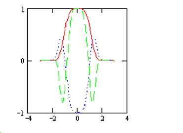
Figure 1. The first three flattened $q=3$ beam modes normalised to unity ($n=0$ continuous, $n=1$ dot, $n=2$ dash). We take $A=1$ and $y=-1$.

The shape is that of the so called flattened optical beams. These beams are different from the usual Gaussian beams since they have flat transverse distribution as shown in Fig. 2 and Fig. 3.

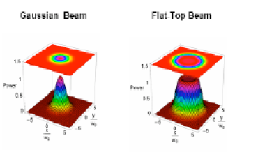
Figure 2. Transverse distribution of a Gaussian and a Flattened beam, the difference in intensities ( denotes the beam waist, with L being the length of the cavity and k the wave vector of the optical field )

The advantage offered by flattened beams with respect to ordinary Gaussians is that they provide larger suppression of thermal noise on the mirror surface because of a better average on the surface fluctuations, they are therefore particularly useful for high power lasers.

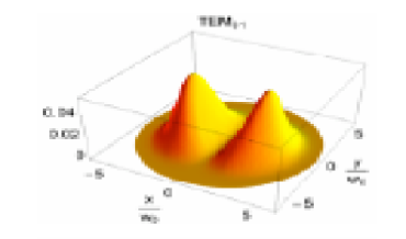
Figure 3. Transverse distribution of a higher order flattened mode

It is evident that if we take a transverse section of the flat top distribution in Figs. 2, 3 we get the distribution similar to that given in Fig. 1 for $n=0$ and $n=1$ respectively [19] used in optics to treat a light beam whose cross section has an intensity as uniform as possible.

A typical example of flattened beam is a super–gaussian

$$f(x)\propto e^{-x^{p}}$$ (99)

whose profile becomes more and more flat as $p$ increases.

It is evident that the function $\Phi_{n}(x,y)$ is a super–gaussian for $n=0$ and that for $n>0$ we have higher order super–gaussian flattened modes.

The distribution of a higher order modes can be obtained from the square moduli of the functions (96) and are shown in Fig. 4 for the cases $n=4$ and $n=30$.

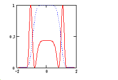
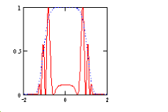
Figure 4. Flattened beam mode distribution $q=3$ (normalized to unity) and comparison with the fundamental. a) $n=4$ ,b) $n=30$

The advantage offered by this family of orthogonal functions is two-fold

a:

They provide the natural set for the expansion of flattened beams

b:

They offer the possibility of treating the higher order modes and not only the fundamental one.

The study of the propagation of the above family of flattened beams can be performed using the set of functions introduced in this article. We postpone this to a forthcoming investigation.

It is worth pointing out that we have

$$\Phi_{n}(x,y)=\alpha_{n}(-y)^{n}e^{-{\frac{{z}}{{2}}}}L_{n}^{(\alpha)}(z)$$ (100)

and we can hence discuss the relevant evolution using $z$ as the independent transverse coordinate.

It is also worth stressing that the operators $\hat{P},\hat{M}$ can be used to form other Lie algebras, different from the Heisenberg one, similarly as $x$ and $p=-i/dx$ are used to form e.g. su(1,1). In turn these are well suited to describe the optical cavity elements and filters exploited to flatten the beam distribution, as it will be shown in a forthcoming investigation.

6.3. Applications in Astrophysics

The Sunyaev–Zeldovich effect [21, 22, 23] is the distorsion of the cosmic microwave background radiation spectrum by the inverse Compton scattering of high energy electrons. When describing this effect the authors [21, 22] obtained the diffusion equation (the Sunyaev–Zeldovich equation):

$$\frac{\partial w}{\partial\tau}=\frac{1}{\xi^{2}}\frac{\partial}{\partial\xi}\xi^{4}\frac{\partial w}{\partial\xi}.$$ (101)

Eq. (101) has a symmetry algebra with basis:

$$X_{1} = \partial_{\tau}-\frac{9}{4}w\partial_{w},$$ (102)

$$X_{2} = \tau\partial_{\tau}+\frac{1}{2}\xi\log\xi\partial_{\xi}-\frac{1}{4}\bigl{[}9\tau+3\log\xi+1\bigr{]}w\partial_{w},$$

$$X_{3} = \tau^{2}\partial_{\tau}+\tau\xi\log\xi\partial_{\xi}-\frac{1}{4}\bigl{[}9\tau^{2}+2\tau+6\tau\log\xi+\log^{2}\xi\bigr{]}w\partial_{w},$$

$$X_{4} = \xi\partial_{\xi}-\frac{3}{2}w\partial_{w},$$

$$X_{5} = \tau\xi\partial_{\xi}-\frac{1}{2}\bigl{[}3\tau+\log\xi\bigr{]}w\partial_{w},$$

$$X_{6} = w\partial_{w}.$$

This Lie algebra is isomorphic to the algebra given in eq. (39), implying that the Sunyaev–Zeldovich equation (101) might be equivalent to the heat equation. Indeed it is and the equivalence is realized by the transformation

$$t=\tau,\quad x=\log\xi,\quad u(x,t)=\xi^{3/2}e^{\frac{9}{4}\tau}w(\xi,\tau),$$ (103)

(see also [24]) If $w(\xi,\tau)$ satisfies eq. (101) then $u(x,t)$ satisfies the heat equation $u_{t}=u_{xx}$. Hence the Sunyaev–Zeldovich equation can be solved in terms of the functions (74) constructed in this article (for $q=1$ and $k_{0}=2At$).

7. CONCLUSIONS

One way of summing up the results of the present article is the following. We have constructed the most general operators $\hat{P},\hat{M}$ of the form (2) that satisfy the Heisenberg relation (4) and used them to construct the monomials $u_{n}(x)=\hat{M}^{n}u_{0}(x)$. They are eigenfunctions of the linear operators $L=\hat{P}\hat{M}$ corresponding to positive integer eigenvalues $\lambda_{n}=n+1$ .

The second order operator $L$ given in eq. (32) is thus factored into a product of 2 operators $\hat{P}$ and $\hat{M}$. The usual factorization of a differential operator is into two lower order differential operators [25, 26]. Ours is highly non standard: a differential operator $\hat{P}$ times an integral one $\hat{M}$.

The functions $u_{n}(x)$ are expressed in terms of generalized Laguerre polynomials $L_{n}^{(\alpha)}(z)$, or equivalently , the confluent hypergeometric function ${}_{2}F_{0}(a,b;z)$. This includes the Hermite polynomials for $\alpha={\frac{{1}}{{2}}}$, or $\alpha=-{\frac{{1}}{{2}}}$ but none of the other classical orthogonal polynomials, related to the hypergeometric function (rather then the confluent one).

There is a good reason for this. We have imposed the form (2) on the operators $\hat{P},\hat{M}$ and the monomiality condition then leads to an eigenvalue problem in which the order of the polynomials $n$ enters in the eigenvalues only and enters linearly. For all other classical orthogonal polynomials the dependence on $n$ is more general.

We are looking into possible generalizations in order to obtain monomial realizations of other classes of orthogonal polynomials. This can e. g. be done by imposing all the properties of monomiality, but allowing $\hat{P},\hat{M}$ to depend on $n$,

$$\hat{P}_{n}u_{n}(x)=n\,u_{n-1}(x),\qquad\hat{M}_{n}u_{n}(x)=u_{n+1}(x).$$ (104)

The Heisenberg relation should in this case be modified to

$$(\hat{P}_{n+1}\hat{M}_{n}-\hat{M}_{n-1}\hat{P}_{n})\,u_{n}(x)=u_{n}(x)$$ (105)

As also stressed in the previous section the possibility of introducing an extra variable makes it possible to consider our polynomials (or functions) as depending on two variables (and also on two parameters $n$, $\alpha$).

A further topic that is being pursued is that of applications, as outlined in Section 6. A very special case of eq. (94) was studied in Ref. [8]. We intend to study eq. (94) in general with $\hat{P},\hat{M}$ as specified in this article, for a wide choice of the functions $F(\hat{P},\hat{M})$.

Regarding applications we have stressed that the form of the introduced orthogonal polynomials is ideally suited for the study of optical flattened beams.

References

- [1] S. Roman and G.C. Rota, The umbral calculus, Adv. Math. 27, 95–188 (1978).
- [2] S. Roman, The Umbral Calculus, Academic Press, New York, 1984.
- [3] G.C. Rota, Finite Operator Calculus, Academic Press, New York, 1975.
- [4] A. Di Bucchianico and D. Loeb, Umbral Calculus. The Electronic Journal of Combinatorics DS3 (2000).
- [5] G. Dattoli, M. Migliorati and H.M. Srivastava, Sheffer polynomials, monomiality principle, algebraic methods and the theory of classical polynomials, Math. Comp. Modelling, 45, 1033–1041 (2007).
- [6] G. Dattoli, A. Torre and G. Mazzacurati, Monomiality and integrals involving Laguerre polynomials, Rend. Mat. Ser. VII, 18, 565–574 (1998).
- [7] P. Blasiak, G. Dattoli, A. Horzela and P.A. Penson, Representations of monomiality principle with Sheffer–type polynomials and boson normal ordering, Phys. Lett. A352, 7–12 (2005).
- [8] G. Dattoli, M. Migliorati and S. Kahn, Solutions of integro–differential equations and operational methods, Appl. Math. Comp 186, 302–308 (2007).
- [9] A.V. Turbiner, Quasi–exactly–solvable problems and sl(2) algebra, Comm. Math. Phys. 118, 467–474 (1988).
- [10] Yu. Smirnov and A.V. Turbiner, Lie algebra discretization of differential equations, Mod. Phys. Lett. A10, 1795–1802 (1995).
- [11] C. Chyssomlokos and A.V. Turbiner, Canonical commutation preserving maps, J. Phys. A 34, 10475–10485 (2001).
- [12] D. Levi, P. Tempesta and P. Winternitz, Umbral calculus, difference equations and the discrete Schrödinger equation, J. Math. Phys. 45, 4077–4105 (2004).
- [13] D. Levi, P. Tempesta and P. Winternitz, Lorentz and Galilei invariance on lattices, Phys. Rev. D 69, 105011, 1–6 (2004).
- [14] P.J. Olver, Applications of Lie groups to differential equations, Springer-Verlag, New York, 1993.
- [15] R. Courant and D. Hilbert, Methods of Mathematical Physics, Wiley, New York, 1989.
- [16] I.S. Gradshteyn and I.M. Ryzhik, Tables of Integrals, Series and Products, Academic Press, New York, 1965.
- [17] M. Abramowitz and I.A. Stegun, Handbook of Mathematical Functions, Dover, New York, 1968.
- [18] B.C. Hall, Lie Groups, Lie Algebras and Representations: An Elementary Introduction, Springer & Verlag, New York, 2003; see also arxiv:math-ph/0005032.
- [19] A.E. Siegman, Laser beams and resonators: Beyond the 1960s, IEEE Journal of Selected Topics in Quantum Electronics 6, 1389 -1399 (2000).
- [20] F. Gori, Flattened Gaussian beams, Opt. Commun. 107, 335–341 (1994).
- [21] R.A. Sunyaev and Ya.B. Zeldovich, Small scale fluctuations of relic radiation, Astrophys. Space Science 7, 3 (1970).
- [22] R.A. Sunyaev and Ya.B. Zeldovich, Microwave background radiation as a probe of the contemporary structure and history of the universe, Ann. Rev. Astron. Astrophys. 18, 537–560 (1980).
- [23] Y. Rephaeli, S. Sadeh, M. Shimon,The Sunyaev Zeldovich effect, Riv. Nuovo Cimento 29(12) 1–18 (2006).
- [24] G. Dattoli, M. Migliorati, K. Zhukovsky, An elementary account of relativistic cosmology, Riv. Nuovo Cimento 29 (10) 1–85 (2006).
- [25] L. Infeld and T.E. Hull, The factorization method, Rev. Mod. Phys. 23, 21–68 (1951).
- [26] B. Mielnik and O. Rosas–Ortiz, Factorization: a little or a great algorithm, J. Phys. A 37, 10007–10035 (2004).