Delay Induced Instabilities in Self-Propelling Swarms

Abstract

We consider a general model of self-propelling particles interacting through a pairwise attractive force in the presence of noise and communication time delay. Previous work by Erdmann, et al. [Phys. Rev. E 71, 051904 (2005)] has shown that a large enough noise intensity will cause a translating swarm of individuals to transition to a rotating swarm with a stationary center of mass. We show that with the addition of a time delay, the model possesses a transition that depends on the size of the coupling amplitude. This transition is independent of the initial swarm state (traveling or rotating) and is characterized by the alignment of all of the individuals along with a swarm oscillation. By considering the mean field equations without noise, we show that the time delay induced transition is associated with a Hopf bifurcation. The analytical result yields good agreement with numerical computations of the value of the coupling parameter at the Hopf point.

The collective motion of multi-agent systems have long been observed in biological populations including bacterial colonies Budrene and Berg (1995); Ben-Jacob et al. (1997); Brenner et al. (1998), slime molds Levine and Reynolds (1991); Nagano (1998), locusts Edelstein-Keshet et al. (1998) and fish Couzin et al. (2002). However, mathematical studies of swarming behavior have been performed for only a few decades. In addition to providing examples of biological pattern formation, the information gained from these mathematical investigations has led to an increased ability to intelligently design and control man-made vehicles Leonard and Fiorelli (IEEE, Piscataway, NJ, 2001); Justh and Krishnaprasad (IEEE, Piscataway, NJ, 2003); D’Orsogna et al. (2006); Morgan and Schwartz (2005); Triandaf and Schwartz (2005).

Many types of mathematical models have been used to describe coherent swarms. One popular approach is based on a continuum approximation in which scalar and vector fields are used to describe all of the relevant quantities Toner and Tu (1995); Edelstein-Keshet et al. (1998); Toner and Tu (1998); Flierl et al. (1999); Topaz and Bertozzi (2004). Another popular approach is based on treating every biological or mechanical individual as a discrete particle Vicsek et al. (1995); Toner and Tu (1998); Flierl et al. (1999); Couzin et al. (2002); Erdmann et al. (2005). Depending on the problem, these individual-based models may be deterministic or stochastic.

Regardless of the type of swarm model being used, one can see the emergence of ordered swarm states from an initial disordered state where individual particles have random velocity directions Vicsek et al. (1995); Toner and Tu (1995, 1998). These ordered states may be translational or rotational in motion, and they may be spatially distributed or localized in clusters.

In particular, it is known that a localized swarm state may transition to a new dynamical region as the system parameters or the noise intensity is changed. For example, it has been shown in Erdmann et al. (2005) that a planar model of self-propelling particles interacting via a harmonic attractive potential in the presence of noise possesses a noise-induced transition whereby the translational motion of the swarm breaks down into rotational motion.

Another aspect of swarm modeling that has not yet been considered is the effect of time delayed interactions arising from finite communication times between individuals. Much attention has been given to the effects of time delays in the context of physiology Mackey and Glass (1977), optics Ikeda (1979), neurons Landsman and Schwartz (2007), lasers Carr et al. (2006), and many other types of systems. The aim of this Letter is to study the effect of a communication time delay on a model of self-propelling individuals that interact through a pairwise attractive force in the presence of noise.

We consider a general two-dimensional (2D) model of a swarm that consists of identical self-propelled particles of unit mass. The model is described by the following evolution equations of motion:

$$\dot{\bm{r}}_{i}={\bm{v}}_{i},$$ (1)

$$\dot{{\bm{v}}}_{i}=(1-|{\bm{v}}_{i}|^{2}){\bm{v}}_{i}-{\bm{V}}_{i}+\xi_{i}(t),$$ (2)

where ${\bm{r}}_{i}(t)$ and ${\bm{v}}_{i}(t)$ are respectively the 2D position and velocity vectors of the $i^{\rm th}$ particle at time $t$. The terms ${\bm{v}}_{i}$ and $-|{\bm{v}}_{i}|^{2}{\bm{v}}_{i}$ define respectively the mechanisms of self-propulsion and frictional drag. Therefore, if the last two terms on the right hand side of Eq. (2) are neglected, the particles will approach an equilibrium speed of $v_{eq}=1$.

The term ${\bm{V}}_{i}$ in Eq. (2) describes the social interaction, or communication, of the $i^{\rm th}$ individual with all of the other individuals. There are many possible choices for ${\bm{V}}_{i}$ (e.g. Morse function, power law function, etc.). As an example, we define ${\bm{V}}_{i}$ as follows:

$${\bm{V}}_{i}=\frac{a}{N}\mathop{\sum\limits_{j=1}^{N}}\limits_{i\neq j}({\bm{r}}_{i}(t)-{\bm{r}}_{j}(t-\tau)),$$ (3)

where $a$ is the particle interaction coupling parameter, $N$ is the number of particles, and $\tau$ is a constant communication time delay. This particular choice of ${\bm{V}}_{i}$ assumes that only pairwise interactions are important. Furthermore, the interaction is purely attractive and grows linearly with the separation between two particles, much like a spring potential.

Lastly, the term $\xi_{i}$ in Eq. (2) describes a stochastic white force of intensity $D$. This noise is independent for different particles, and is characterized by the following correlation functions:
$\ \langle\xi_{i}(t)\rangle=0,\ \ \langle\xi_{i}(t)\xi_{j}(t)\rangle=2D\delta(t-t^{\prime})\delta_{ij}$.

We numerically integrate Eqs. (1)-(3) using a stochastic fourth-order Runge-Kutta scheme with a constant time step size of $0.001$. To achieve a traveling, localized swarm state, we used constant initial conditions not (a) and switched on the noise after a short amount of time had passed.

It was shown in Erdmann et al. (2005) that the model described by Eqs. (1)-(3) with $\tau=0$ (i.e. no time delay) possesses a noise-induced transition whereby a large enough noise intensity causes a translating swarm of individuals to transition to a rotating swarm with a stationary center of mass, where the center of mass is defined as ${\bm{R}}(t)=(1/N)\sum_{i}{\bm{r}}_{i}(t)$.

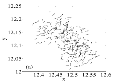
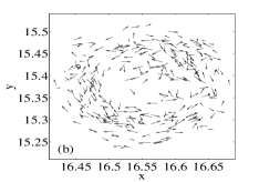
Figure 1: Snapshot of (a) a translating swarm (taken at $t=18$), and (b) a rotating swarm (taken at $t=40$), with $a=100$, $N=300$, $\tau=0$, and $D=0.08$.

Figures 1(a) and 1(b) show snapshots of a swarm at $t=18$ and $t=40$ respectively, with $a=100$, $N=300$, $\tau=0$, and $D=0.08$. The noise was switched on at $t=10$. One can see that the translating swarm [Fig. 1(a)] has undergone a noise-induced breakdown to become a rotating swarm [Fig. 1(b)]. For these values of $a$ and $N$, if a noise intensity of $D<0.054$ is used, then the swarm will continue to translate and it will not transition to a rotational state not (b).

Regardless of which state the swarm is in (translating or rotating), the addition of a communication time delay leads to another type of transition. This transition occurs if the coupling parameter, $a$, is large enough. As an example, we consider a swarm that has already undergone a noise-induced transition to a rotational state before switching on the communication time delay.

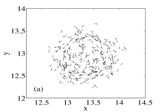
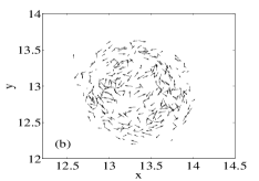
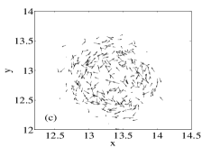
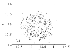
Figure 2: Snapshots of a swarm taken at (a) $t=50$, (b) $t=100$, (c) $t=300$, and (d) $t=600$, with $a=2$, $N=300$, and $D=0.08$. The swarm was in a rotational state when the time delay of $\tau=1$ was switched on at $t=40$.

Figures 2(a)-2(d) show snapshots of a swarm at $t=50$, $t=100$, $t=300$, and $t=600$ respectively, with $a=2$, $N=300$, $\tau=1$, and $D=0.08$. The noise was switched on at $t=10$, and since the noise intensity, $D$, is high enough, the noise caused the swarm to transition to a rotating state [similar to the one shown in Fig. 1(b)]. With the swarm in this stationary, rotating state, the communication time delay was switched on at $t=40$. One can see that for these values of time delay and coupling parameter there is no qualitative change in the stationary, rotating swarm state.

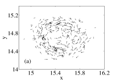
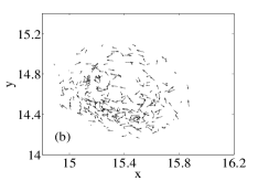
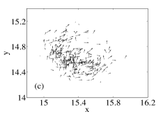
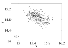
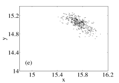
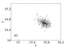
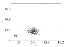
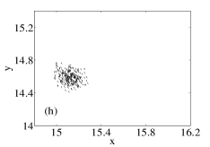
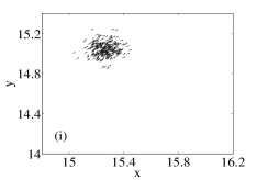
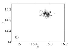
Figure 3: Snapshots of a swarm taken at (a) $t=50$, (b) $t=60$, (c) $t=62$, (d) $t=64$, (e) $t=66$, (f) $t=68$, (g) $t=70$, (h) $t=72$, (i) $t=74$, and (j) $t=76$, with $a=4$, $N=300$, and $D=0.08$. The swarm was in a rotational state when the time delay of $\tau=1$ was switched on at $t=40$.

In contrast to this, Figs. 3(a)-3(j) show snapshots of a swarm at $t=50$, $t=60$, $t=62$, $t=64$, $t=66$, $t=68$, $t=70$, $t=72$, $t=74$, and $t=76$ respectively. As in the previous case, $N=300$, $\tau=1$, $D=0.08$, the noise was switched on at $t=10$ (causing the swarm to transition to a stationary, rotating state), and once in this rotating state, the time delay was switched on at $t=40$. The only difference is that now the value of the coupling parameter is $a=4$. One can see that with the evolution of time, the individual particles become aligned with one another and the swarm becomes more compact. Additionally, the swarm is no longer stationary, but has begun to oscillate [Figs. 3(g)-3(j)]. This clockwise oscillation can more clearly be seen in Fig. 4, which consists of the center of mass, ${\bm{R}}$, of the stationary, rotating swarm at $t=40$ (denoted by a “cross” marker) along with snapshots of the oscillating swarm taken at $t=90.2$, $t=90.6$, $t=91.0$, and $t=91.4$.

This compact, oscillating aligned swarm state looks similar to a single “clump” that is described in D’Orsogna et al. (2006). However, where each “clump” of D’Orsogna et al. (2006) contains only some of the total number of swarming particles, our swarm contains every particle. Additionally, while a deterministic model along with global coupling is used to attain the “clumps” of D’Orsogna et al. (2006), our oscillating aligned swarm is attained with the use of noise and a time delay.

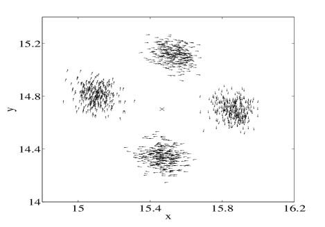
Figure 4: Motion of the oscillating swarm about the center of mass of the stationary, rotating swarm. The oscillating swarm is shown at $t=90.2$ (left), $t=90.6$ (top), $t=91.0$ (right), and $t=91.4$ (bottom). The location of the center of mass of the swarm (at $t=40$) is denoted with a “cross” marker (center).

As we have shown, once the stochastic swarm is in the stationary, rotating state, the addition of a time delay induces an instability. At this point, the stochastic perturbations have a minimal effect on the swarm. Therefore, we will investigate the stability of the stationary, rotating swarm state by deriving the mean field equations without noise. The coordinates $x_{i}$ and $y_{i}$ of each particle in the swarm can be written as follows:

$$x_{i}=X+\delta x_{i}\ \ \ {\rm and}\ \ \ y_{i}=Y+\delta y_{i},$$ (4)

where $X$ and $Y$ are the coordinates of the center of mass, ${\bm{R}}$, of the swarm. Substitution of Eq. (4) into the second-order differential equation that is equivalent to Eqs. (1)-(3) gives an evolution equation for each $x_{i}$ and $y_{i}$. Summing all $i$ of these equations, using the fact that

$$\frac{1}{N}\sum\limits_{i=1}^{N}x_{i}(t)=X(t)\ \ \ {\rm and}\ \ \ \frac{1}{N}\sum\limits_{i=1}^{N}y_{i}(t)=Y(t),$$ (5)

and ignoring all fluctuation terms, leads to the following zero-order mean field equations for the center of mass:

$$\ddot{X}(t)=[(1-\dot{X}^{2})\dot{X}-\dot{X}\dot{Y}^{2}](t)-a(X(t)-X(t-\tau)),$$ (6)

$$\ddot{Y}(t)=[(1-\dot{Y}^{2})\dot{Y}-\dot{Y}\dot{X}^{2}](t)-a(Y(t)-Y(t-\tau)).$$ (7)

The steady state is given by $\dot{X}(t)=\dot{Y}(t)=0$, $X(t)=X(t-\tau)$, and $Y(t)=Y(t-\tau)$. Consideration of small disturbances about the steady state allows one to determine the linear stability. The characteristic equation associated with the linearization of Eqs. (6)-(7) is

$$\lambda(1-\lambda)+ae^{-\lambda\tau}-a=0,$$ (8)

where the exponential term ${\rm exp}(-\lambda\tau)$ is due to the time delay in the governing equations. Since Eq. (8) is transcendental (which is often the case for delay differential equations), there exists the possibility of an infinite number of solutions.

Our numerical simulations indicate the existence of a supercritical Hopf bifurcation as the value of the coupling parameter, $a$, is increased (Figs. 2-4). We identify the Hopf bifurcation point by choosing the eigenvalue to be purely imaginary. Then our choice of $\lambda=i\omega$ is substituted into Eq. (8). The separation of Eq. (8) into real and imaginary parts leads to an equation for the frequency, $\omega$, along with an equation for the value of $a$ at the Hopf bifurcation point. The two equations are

$$\omega^{2}+\omega\cot{(\omega\tau)}-\omega\csc{(\omega\tau)}=0,$$ (9)

$$a_{H}=\frac{\omega}{\sin{(\omega\tau)}}.$$ (10)

Given a specific value of $\tau$, Eq. (9) can be solved numerically for $\omega$. These values of $\tau$ and $\omega$ can then be substituted into Eq. (10) to determine the value of $a$ at the Hopf point.

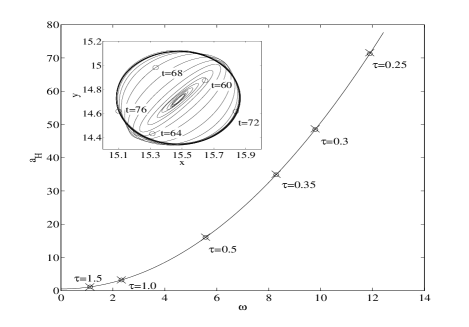
Figure 5: Comparison of analytical (solid line) and numerical (“cross” markers) values of $a_{H}$ and $\omega$ for several choices of $\tau$. The analytical result is found using Eqs. (9)-(10), while the numerical result is found using a continuation method Engelborghs et al. (2001) for Eqs. (6)-(7). The inset shows the stochastic trajectory of the center of mass of the swarm from $t=45$ to $t=90$ for the example shown in Fig. 3.

Figure 5 shows an excellent comparison of the analytical result given by Eqs. (9)-(10) with a numerical result which was found using a continuation method Engelborghs et al. (2001) for Eqs. (6)-(7) for several choices of $\tau$. Furthermore, for $\tau=1$, the value of $a$ at the bifurcation point is $a_{H}\approx 3.2$. This value of $a_{H}$ corresponds very well to the change in behavior of the stochastic swarm that was seen as the value of the coupling parameter was increased from $a=2$ to $a=4$ (Figs. 2-3).

More evidence of the Hopf bifurcation is seen in the inset of Fig. 5. The inset shows the stochastic trajectory of the center of mass of the swarm from $t=45$ to $t=90$ for the example shown in Fig. 3. Once the time delay is switched on at $t=40$ (with the swarm located at the center of the inset figure), the swarm begins to oscillate. The swarm moves along an elliptical path [the position of its center of mass is denoted at several times that correspond to Figs. 3(b), 3(d), 3(f), 3(h), and 3(j)], until it eventually converges to the circular limit cycle.

To summarize, we studied the dynamics of a self-propelling swarm in the presence of noise and a constant communication time delay and prove that the delay induces a transition that depends upon the size of the interaction coupling coefficient. Although our analytical and numerical results were obtained using a model with linear, attractive interactions, the analysis may be applied to models with more general forms of social interaction (these results will appear elsewhere).

Our results provide insight into the stability of complex systems comprised of individuals interacting with one another with a finite time delay in a noisy environment. Furthermore, the results may prove to be useful in controlling man-made vehicles where actuation and communication are delayed, as well as in understanding swarm alignment in biological systems.

We gratefully acknowledge support from the Office of Naval Research and the Army Research Office. E.F. is supported by a National Research Council Research Associateship. The authors benefitted from the valuable comments and suggestions of anonymous reviewers.

References

- Budrene and Berg (1995) E. O. Budrene and H. C. Berg, Nature (London) 376, 49 (1995).
- Ben-Jacob et al. (1997) E. Ben-Jacob, I. Cohen, A. Czirók, T. Vicsek, and D. L. Gutnick, Physica A 238, 181 (1997).
- Brenner et al. (1998) M. P. Brenner, L. S. Levitov, and E. O. Budrene, Biophys. J. 74, 1677 (1998).
- Levine and Reynolds (1991) H. Levine and W. Reynolds, Phys. Rev. Lett. 66, 2400 (1991).
- Nagano (1998) S. Nagano, Phys. Rev. Lett. 80, 4826 (1998).
- Edelstein-Keshet et al. (1998) L. Edelstein-Keshet, J. Watmough, and D. Grünbaum, J. Math. Biol. 36, 515 (1998).
- Couzin et al. (2002) I. D. Couzin, J. Krause, R. James, G. D. Ruxton, and N. R. Franks, J. Theor. Biol. 218, 1 (2002).
- Leonard and Fiorelli (IEEE, Piscataway, NJ, 2001) N. E. Leonard and E. Fiorelli, in Proceedings of the 40th IEEE Conference on Decision and Control (IEEE, Piscataway, NJ, 2001), pp. 2968–2973.
- Justh and Krishnaprasad (IEEE, Piscataway, NJ, 2003) E. W. Justh and P. S. Krishnaprasad, in Proceedings of the 42nd IEEE Conference on Decision and Control (IEEE, Piscataway, NJ, 2003), pp. 3609–3614.
- D’Orsogna et al. (2006) M. R. D’Orsogna, Y. L. Chuang, A. L. Bertozzi, and L. S. Chayes, Phys. Rev. Lett. 96, 104302 (2006).
- Morgan and Schwartz (2005) D. S. Morgan and I. B. Schwartz, Phys. Lett. A 340, 121 (2005).
- Triandaf and Schwartz (2005) I. Triandaf and I. B. Schwartz, Math. Comp. Simulat. 70, 187 (2005).
- Toner and Tu (1995) J. Toner and Y. Tu, Phys. Rev. Lett. 75, 4326 (1995).
- Toner and Tu (1998) J. Toner and Y. Tu, Phys. Rev. E 58, 4828 (1998).
- Flierl et al. (1999) G. Flierl, D. Grünbaum, S. Levin, and D. Olson, J. Theor. Biol. 196, 397 (1999).
- Topaz and Bertozzi (2004) C. M. Topaz and A. L. Bertozzi, SIAM J. Appl. Math. 65, 152 (2004).
- Vicsek et al. (1995) T. Vicsek, A. Czirók, E. Ben-Jacob, I. Cohen, and O. Shochet, Phys. Rev. Lett. 75, 1226 (1995).
- Erdmann et al. (2005) U. Erdmann, W. Ebeling, and A. S. Mikhailov, Phys. Rev. E 71, 051904 (2005).
- Mackey and Glass (1977) M. C. Mackey and L. Glass, Science 197, 287 (1977).
- Ikeda (1979) K. Ikeda, Opt. Commun. 30, 257 (1979).
- Landsman and Schwartz (2007) A. S. Landsman and I. B. Schwartz, Nonlinear Biomed. Phys. 1, 2 (2007).
- Carr et al. (2006) T. W. Carr, I. B. Schwartz, M.-Y. Kim, and R. Roy, SIAM J. Appl. Dyn. Syst. 5, 699 (2006).
- not (a) Although any constant value for the initial position and velocity may be used, we have arbitrarily chosen the following initial conditions: .
- not (b) The critical noise intensity value reported in this article results from the use of a stochastic numerical solver that is of higher order than the one used in Ref. Erdmann et al. (2005), along with a Gaussian noise distribution.
- Engelborghs et al. (2001) K. Engelborghs, T. Luzyanina, and G. Samaey, Tech. Rep. TW 330, Department of Computer Science, Katholieke Universiteit Leuven (2001); http://www.cs.kuleuven.ac.be/publicaties/rapporten/ tw/TW330.abs.html.