The evolution of Hii galaxies: Testing the bursting scenario through the use of self-consistent models

Abstract

We have computed a series of realistic and self-consistent models of the emitted spectra of Hii galaxies. Our models combine different codes of chemical evolution, evolutionary population synthesis and photoionization. The emitted spectrum of Hii galaxies is reproduced by means of the photoionization code CLOUDY, using as ionizing spectrum the spectral energy distribution of the modelled Hii galaxy, which in turn is calculated according to a Star Formation History (SFH) and a metallicity evolution given by a chemical evolution model that follows the abundances of 15 different elements. The contribution of emission lines to the broad-band colours is explicitly taken into account.

The results of our code are compared with photometric and spectroscopic data of Hii galaxies. Our technique reproduces observed diagnostic diagrams, abundances, equivalent width-colour and equivalent width-metallicity relations for local Hii galaxies.

1 Introduction

Hii galaxies, a subset of Blue Compact Galaxies (BCG), are gas rich dwarf galaxies whose optical spectra are dominated by strong and narrow emission lines. They are currently experiencing intense star formation in small volumes. The emission lines are produced by gas ionized by the young massive stars. Observations indicate that Hii galaxies are in general metal poor systems. This fact in addition to their very young stellar populations has been known for some time and has led to the proposal that these systems are very young, suffering their first burst of star formation (Sargent & Searle, 1970).

It seems, however, that these galaxies are not as young as it was originally thought, since recent photometric observations indicate that they host stellar populations which are at least $10^{7}-10^{8}$ a. old, reaching in some cases a few Ga (Telles et al., 1997; Legrand, 2000; Tolstoy, 2003; Cairós et al., 2003; , van Zee et al.2004; Thuan & Izotov, 2005). There is now wide agreement about the existence of underlying populations with ages of several Gas in BCGs and/or Hii galaxies. Even in the most metal-poor galaxy known, Izw18, the best candidate to primordial galaxy, there is an underlying population of at least some 10⁸–10⁹ a (Izotov & Thuan, 2004).

However there is no consensus about their history of star formation. Two scenarios are postulated:

a) The star formation takes place in short but intense episodes separated by long quiescent periods of null or low activity (Bradamante et al., 1998).

b) The star formation is continuous and of low intensity along the galaxy life, with superimposed sporadic bursts (Legrand, 2000).

In both scenarios, a stellar population of intermediate age contributes to the observed luminosity. Indeed, recent work takes into account the existence of an underlying stellar population and combine photo-ionization codes with evolutionary synthesis models (hereinafter ESM). Examples of this procedure can be found in Garnett et al. (1999), Mas-Hesse & Kunth (1999), (Stasińska & Izotov2003) and (Moy et al.2001). In general the ESM so far do not include the chemical evolution. Given the low metal content of Hii galaxies the metallicity effect can be of considerable relevance.

(Terlevich et al.2004) have shown that the equivalent width of the H$\beta$ line, EW(H$\beta$), which can be taken as an age indicator for the ionizing population, and the (U-V) colour in Hii galaxies show an anti-correlation which cannot be interpreted in terms of a single stellar population (SSP). At a given EW(H$\beta$) the data are displaced to colours redder than those predicted by the models. The most likely explanation is that the ionizing population, that is the most recent burst of star formation, is overimposed on an older stellar population evolved enough as to produce a redder (U-V) colour. There is also an inverse correlation between EW(H$\beta$) and the gas oxygen abundance, $12+log(O/H)$, which could be interpreted in terms of galactic chemical evolution: as the average age and the total mass of the stellar population increases , the EW(H$\beta$) decreases and the mean metallicity of the interstellar medium increases.

A number of works (Shiet al., 2006, and references therein) have computed purely chemical evolution models (hereinafter CEM) for the study of BCG and dwarf irregular galaxies. Most of them assume that the star formation occurs in bursts and include the effects of galactic winds and/or gas infall. However most of them limit the study to the evolution of nitrogen and oxygen abundances (Henry et al., 2000; Larsen et al., 2001) and/or the luminosity-metallicity relation (Mouhcine & Contini, 2002). Only (Vázquez et al.2003) used the information coming from the chemical evolution models from Carigi et al. (2002) to perform the next step and combine chemical and spectral evolution. Their models exclude however the early stages of evolution, i.e. during the nebular stage when the most massive stars dominate the energy output.

A code combining chemical evolution, evolutionary synthesis and photo-ionization models has not yet been developed and used for the spectral analysis of BCG and Hii galaxies.

In this work, we include the chemical evolution model results in the computation of the spectral energy distributions which are used as ionizing source for a photo-ionization code.

Our method allows the simultaneous use of the whole available information for the galaxy sample concerning on the one hand the ionized gas – emission lines intensities and equivalent widths, elemental abundances, gas densities – which defines the present time state of the galaxy, and on the other hand spectro-photometric parameters – colours, absorption spectral indices — defined by the stellar populations and their evolution with time and thus related to the galaxy star formation history. This is done in a self-consistent way, that is using the same assumptions regarding stellar evolution, model stellar atmospheres and nucleosynthesis, and using a realistic age-metallicity relation.

The basic codes employed are described in Section 2. Section 3 shows the corresponding results of each kind of model, and the whole combined results about galaxy evolution. These results are discussed in Section 4. Finally, our conclusions are summarized in Section 5.

2 Model description

2.1 Chemical evolution

The code used for this work is a generalization of the code used for the Solar Neighborhood by Ferrini et al. (1992) and applied to the whole Galaxy disc in Ferrini et al. (1994). That model described the galaxy as a two-zone system (halo and disc) in which the disc is a secondary structure formed by the gravitational accumulation of gas from the halo. In the present work, however, all the gas is assumed to be within an only region from $t=0$, that is, the collapse time scale has been eliminated as an input parameter of the code. The matter is assumed to be in different phases:

• A stellar population, where we distinguish the stars able to create and eject heavy elements to the interstellar medium ($M>4M_{\odot}$), and the stars which only eject hydrogen and He ($M<4M_{\odot}$).

• Stellar remnants, as the endpoint of star evolution, that act as a matter sink, removing mass from chemical evolution.

• Interstellar diffuse gas out of which stars are forming following a simple Schmidt law. No molecular component is explicitly considered in the present work.

A bursting star formation has been assumed taking place in successive bursts along the time evolution. At any time, the available gas for each burst is the sum of the gas left after the previous burst of star formation and the gas ejected by massive stars.

According to this description, the time dependence of the total mass fraction in each phase and the chemical abundances in the ISM are determined by the interactions between these phases and, as a consequence of the evolution, we get the star formation rate. The basic equations to study the behavior of the mass of stars and gas are, therefore:

$$\frac{dM}{dt} = 0$$ (1)

$$\frac{dM_{s}}{dt} = \Psi-E$$ (2)

$$\frac{dM_{g}}{dt} = -\Psi+E$$ (3)

$$M = M_{s}+M_{g}$$ (4)

where $\rm M_{s}(t)$ is the mass in stars, M_g(t) is the mass of gas, $M$ is the total mass of the system, $\Psi$(t) the star formation rate and E(t) the ejection rate of mass from the stars to the ISM. A part of the restituted gas consists of enriched material, E_Z(t), which is created in the interior of the stars and is ejected when they die. To compute both quantities, ejected gas and element production, we use the $Q_{ij}$ matrix formalism introduced by Talbot & Arnett (1973) and widely used in classical chemical evolution models. It is very useful to treat elemental abundances which increase at different rate in the interstellar medium, that is, the non-solar elemental ratios (Portinari et al., 1998). In the present work we adopt the same matrix prescription as in Gavilán et al. (2006), which is an updated version from the one given in Ferrini et al. (1992) and Galli et al. (1995) calculated following the method described by Portinari et al. (1998).

In order to calculate these matrices it is necessary to consider the nucleosynthesis of stars, their initial mass function (IMF) and their end either as type I or II supernovae, or through quiet evolution. The mean stellar lifetimes, final states, and nucleosynthesis products, depend on the stellar mass which makes the IMF to play an important role in the chemical evolution model. The adopted IMF is assumed to be universal in space and constant in time (Wyse, 1997; Scalo, 1998; Meyer et al., 2000) and taken from Ferrini et al. (1990). This IMF is very similar to Scalo’s law (Scalo, 1986) and in good agreement with the recent expressions from Kroupa (2001) and Chabrier (2003). Nucleosynthesis yields for massive stars have been taken from Woosley & Weaver (1995). For low and intermediate mass stars, we have used the yields from Gavilán et al. (2005). The combination of these sets of stellar yields, with our assumed IMF producing the required yields per stellar generation, has been completely revised and calibrated with the MWG in Gavilán et al. (2005, 2006), where other stellar yields sets have been used and analyzed too. It also reproduces observations of spiral and irregular galaxies (Mollá & Díaz, 2005), obtaining reasonable results even for nitrogen abundances in low-metallicity objects (Mollá et al., 2006). For type I supernova explosion releases, model W7 from (Nomoto et al.1984), as revised by Iwamoto et al. (1999), has been taken, while the rate of this type of SNIa explosions are included through a table given by Ruiz-Lapuente (private communication), following works of Ruiz-Lapuente et al. (2000).

We have assumed that the gas is used to form stars with a given efficiency called H: $\Psi=H\cdot M_{g}$. If there would not be gas ejection from massive stars, as it would be the case for instance in the firsts moments of the evolution, $(E=0)$, then:

$$\frac{dM_{s}}{dt} = HM_{g}$$ (5)

$$\frac{dM_{g}}{dt} = -HM_{g}$$ (6)

That is, the consumed gas rate would be a function that depends on the available gas at a given time, being a decreasing function of time through the parameter H, which defines the star formation efficiency. Then:

$$\frac{dM_{g}}{M_{g}}=-Hdt\Rightarrow M_{g}(t)=M_{g0}e^{-Ht}$$ (7)

A change in the star formation rate implies a change in the value of the parameter H or efficiency:

$$H=\frac{ln\frac{M_{g,0}}{M_{g}}}{\Delta t}$$ (8)

We have run models considering the star formation as a set of successive bursts in a region with a total mass of gas of 100$\cdot$10⁶ M_⊙ and a radius of 500 pc (see section 3.2 for details). Every galaxy experiences 11 star formation bursts along its evolution of 13.2 Ga, that is one every 1.3 Ga. In each burst a certain amount of gas is consumed to form stars. We have computed two types of models. In the first one, which we call burst models (models B), the same efficiency H is assumed for every burst while in the second one (models A) we assume an attenuated bursting star formation mode , i. e. a variable H is assumed along the time evolution. For each type we have computed two models with different initial star formation efficiency:

1. model 1, that uses $\sim$ 64 per cent of the gas for star formation in each time step. Thus, following Eq.(8), $1/H=0.5$ Ma

2. model 2, that uses $\sim$ 33 per cent of the gas to form stars in each time step, which implies $1/H=1.25$ Ma

These percentages are maintained in models B, which means that every burst will transform the corresponding percentage of the available gas (taking into account the gas ejected by massive stars) in stars. In Models A, these values correspond to the initial efficiencies and are reduced in the successive bursts by a factor $n$, where $n$ is the number of the burst.

The code solves the chemical evolution equations to obtain, in each time step, the abundances of 15 elements: H, D, $\rm{}^{3}He$, $\rm{}^{4}He$, C, $\rm{}^{13}C$, O, N, Ne, Mg, Si, S, Ca, Fe, and nr where nr are the isotopes of the neutron rich elements, synthesized from $\rm{}^{12}C$, $\rm{}^{13}C$, ¹⁴N and $\rm{}^{16}O$ inside the CO core. We have taken a time step, $\Delta$t= 0.5 Ma , from the initial time, $t=0$, up to the final one, $t=13.2$ Ga. Also, at each time step, the star formation rate and the mass in each phase – low mass, massive stars and remnants, total mass in stars created, and mass of gas– are computed. This amounts to a total of 26348 stellar generations or SSPs, each one with its corresponding age and metallicity.

2.2 Evolutionary synthesis

Once the chemical evolution models have been calculated, the spectrophotometric properties can also be obtained. In this work we have used the code from García-Vargas et al. (1995a, b, 1998) as updated in Mollá & García-Vargas (2000). The required inputs are the stellar isochrones and the stellar atmosphere models for the individual stars. In that work we used the set of 50 isochrones from the Padova group from Bertelli et al. (1994) for ages between 4 Ma and 20 Ga, for 5 metallicities between 1/50 and 2.5 Z_⊙ (Z$=$0.0004, 0.004, 0.008, 0.02 and 0.05). To this set of isochrones we have added other 18 isochrones from Bressan et al. (1993) and Fagotto et al. (1994) with ages from 0.5 to 4 Ma, used in García-Vargas et al. (1995a) and García-Vargas et al. (1998) for the youngest stellar populations of 4 metallicities Z$=$0.004, 0.008, 0.02 and 0.05. That means that for the lowest metallicity, $Z=0.0004$, only isochrones older than 4 Ma are available.

In both cases, isochrones give the number of stars in each phase assuming that stellar clusters were formed with a standard Salpeter IMF with $m_{low}=0.6$ M_⊙ and m${}_{up}=100$ M_⊙. This IMF, although using the same lower and upper limits, is not exactly the one used in the multiphase chemical evolution code, what implies some differences in the resulting spectra, mainly for the oldest and the youngest stellar populations. They are, however, smaller than 10 per cent (García-Vargas et al. 2008, in preparation), and therefore we assume that this inconsistency will not produce very important differences in the final results.

The emergent spectral energy distribution (SED) was synthesized by calculating the number of stars in each point of the H-R diagram and assigning to it the most adequate stellar atmosphere model. The models of Clegg & Middlemass (1987) and Lejeune et al. (1997) have been used for stars with $T_{eff}\geq$ 50000 K (last evolutionary stages of massive stars) and 2500 $\leq T_{eff}<50000$ K, respectively.

To each SED computed for a stellar cluster, it was added a continuum nebular emission contribution as explained in García-Vargas et al. (1998). The gas is assumed to have an electron temperature, T_e which depends on Z. The assumed values are T${}_{e}=$18000, 11000, 9000, 6500 and 4000 K for Z$=$0.0004, 0.004, 0.008, 0.02 and 0.05, respectively, selected according to the average value obtained by García-Vargas et al. (1995b). The free-free, free-bound emission by hydrogen and neutral helium, and the two photon hydrogen-continuum have been calculated by means of the atomic data from Aller (1984) and Ferland (1980).

The SEDs for the complete sets of 68 (50 for Z=0.0004) isochrones were calculated with the same code as in Mollá & García-Vargas (2000) for the cited metallicities. Therefore we finally have a set of 68 SEDs for SSP of different ages for 4 metallicities each, and 50 for ages older than 4 Ma for Z$=$0.0004, which we use as a spectral library.

Once the SEDs for SSPs are computed, they must be convolved with the star formation history (SFH) in order to calculate the corresponding SED for a region where more than a burst take place:

$$L_{\lambda}(t)=\int^{t}_{0}S_{\lambda}(\tau,Z(t^{\prime}))\Psi(t^{\prime})dt^{\prime}$$ (9)

where $\tau=t-t^{\prime}$ is the age of the stellar population created in a time $t^{\prime}$ and $S_{\lambda}$ being the SED for each SSP of age $\tau$ and metallicity Z reached in that time $t^{\prime}$. A SED from the SSP library, $S_{\lambda}$, must assigned to each time step according to its corresponding age and metallicity taking into account the SFH, $\Psi(t)$, and the AMR, $Z(t)$, obtained from the chemical evolution model, to finally calculate L${}_{\lambda}(t)$ by the above integration. However the metallicity changes continuously while the available SEDs have only 4 or 5 possible values. We have, therefore, interpolated logarithmically between the two SSP of the same age $\tau$ closest in metallicities to Z(t’) to obtain the corresponding $S_{\lambda}(\tau,Z(t^{\prime}))$. The final result is the total luminosity at each wavelength $\lambda$.

When this process is applied to the stellar population created by the first burst two problem arise. On the one hand the initial metallicity is Z$=0$ and, although during the first Ma after the creation of the first stars the metallicity increases, it does not reach the minimum Z$=$0.0004, and therefore we must extrapolate with the available SEDs of the youngest SSPs. Due to the uncertainties in the evolution of the quasi-zero-metallicity stars, we have preferred to assign to this first burst metallicity a minimum value of 0.0028, smaller than the one reached at the end of the first burst but still valid for extrapolating without creating instability numerical problems. On the other hand we must to use two different pairs of metallicities to extrapolate with the SEDs of SSPs: Z$=$0.004 and 0.008 before 4 Ma and Z$=$0.0004 and 0.004 after 4 Ma, since SEDs for the most-metal-poor and youngest SSPs are not available. We have checked that this method does not produce discontinuities and that the resulting spectra behave smoothly. In this way we obtain the SED corresponding to the whole stellar population, including the ionizing continuum proceeding from the last formed stellar population.

2.3 Photo-ionization

The photo-ionization code CLOUDY, in its 96.0 version (Ferland et al., 1998), has been used in order to obtain the emission lines. The gas is assumed to be ionized by the massive stars belonging to the current burst of star formation whose SED has been previously calculated by the combination of the chemical and evolutionary synthesis models. The shape of the ionizing continuum is defined by the pair of values ($\nu$(Ryd), log$\nu L_{\nu}$) (Eq. 9).

We have assumed the emitting gas to be located at a distance $\rm R=500$ pc at the beginning of the evolution. This size is characteristic of Hii galaxies (Telles et al., 1997). This radius is subsequently adjusted as to keep a constant stellar density configuration. This results in all cases in a plane-parallel geometry.

A given model is characterized by its ionization parameter U defined as:

$$U=Q(H)/4\pi cn_{H}R^{2}$$ (10)

where n_e is the electron density, assumed constant for simplicity and equal to 100 cm^-3, and $Q(H)$ is the number of Lyman ionizing photons, calculated from the cluster SED, which reach the gas at a velocity $c$. Finally, the gas elemental abundances are those reached at the end of the starburst previous to the current one, as calculated from the chemical evolution model, except for Na, Ar and Ni which are not computed in the model and are scaled to the solar ratio (Asplund et al., 2005).

3 Results

3.1 Chemical evolution

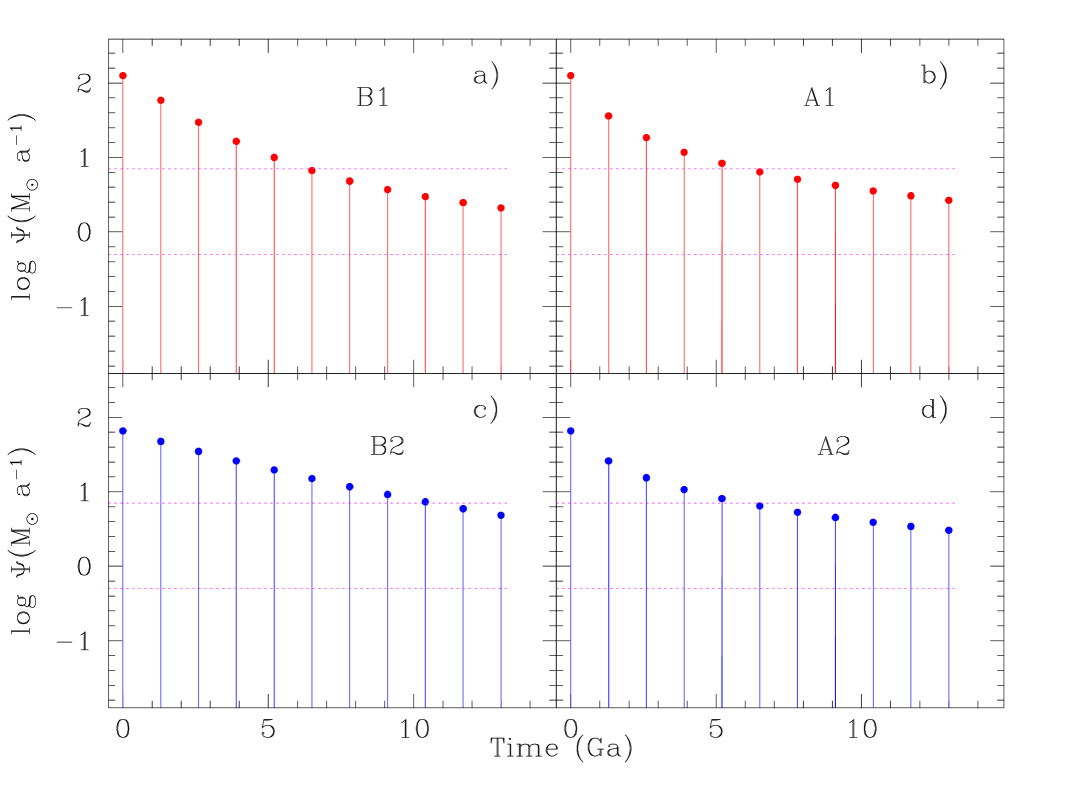
Figure 1: Star formation history for: a) burst model 1 (B1); b) attenuated burst model 1 (A1); c) burst model 2 (B2); and d) attenuated burst model 2 (A2). Dotted lines represent the upper and lower limits to the SFR estimated for BCG and/or Hii galaxies by Hoyos et al. (2004).

3.1.1 Star formation rates

The star formation rate is one of the main results of the different models since it drives the behaviour of all the other quantities. In Fig. 1 the star formation history for each of the 4 computed models is shown. In all of them the first burst is strong, while the successive bursts are less intense since the amount of gas available has decreased in spite of the ejected gas produced by the massive stars. In models A (right panels), the first burst has the same star formation rate as in Models B (left panels), since the initial efficiency is the same for both. The successive star formation episodes have a smaller star formation rate in models A than the corresponding ones in models B due to the attenuation factor included in the inputs.

Hoyos et al. (2004) have estimated the star formation rates for the sample of 39 local Hii galaxies of different morphologies from Telles et al. (1997), which were selected from the most luminous of the Terlevich et al. (1991) catalog and with H$\beta$ equivalent widths between 30 and 280 Å . These star formation rates were obtained from the H$\alpha$ luminosity, by assuming T${}_{e}=10^{4}$ K and case B recombination. They are in the range from 0.5 to 7 M${}_{\odot}a^{-1}$, marked by dotted lines in Fig. 1, indicating that these Hii galaxies have high star formation rates. These findings are in agreement with those from (Taylor et al.1994) who found star formation rates in the range of 10^-4 to 10 M${}_{\odot}a^{-1}$. Our models produce SFR between the observed values after the sixth burst, which corresponds to 6.5 Ga after the beginning of star formation, except model B2, where every burst before the ninth-tenth show higher SFR than observed.

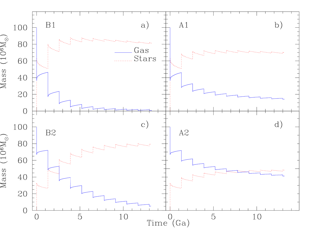
Figure 2: Time evolution of the gas and star mass for models: a) B1; b) A1; c) B2; and d) A2.

Since the star formation consumes gas, the averaged gas mass decreases with time following Eq.(6), as can be seen in Fig. 2. The chemical evolution code, however, takes into account the mass of gas ejected from massive stars during their evolution and, therefore, the gas mass increases during a given burst. On the other hand, the mass of stars which increases in each burst and globally due to the star formation, decreases during each burst as the most massive stars end their lives. It is interesting to note that models with smaller efficiencies, H, in the lower panels of Figs. 1 and 2, consume less gas in each burst and, as a consequence, the star formation rate remains higher, and declines more slowly, than in models with higher values of H shown in the upper panels.

3.1.2 Elemental abundances

The element content of the gas is usually measured through the oxygen abundance, given as $\ 12+log(O/H)$. Oxygen contributes more than 40 per cent to the mass in metals and is mainly created within massive stars. Since these stars are very short lived, their products are ejected very rapidly to the interstellar medium (ISM) and hence the value of its oxygen abundance increases with time, as shown in Fig. 3. In that figure we see how O/H increases abruptly when a burst takes places remaining more or less constant between each two of them.

Observational data from Terlevich et al. (1991) and Hoyos & Díaz (2006) show that most of the Hii galaxies have metallicity distributions between $\rm 7.5<12+log(O/H)<8.5$. These limits are shown as dashed lines in Fig. 3. The first limit is reached with the first burst in all cases. It can be seen that models of type 1 (dotted lines) show oxygen abundances higher than the observed upper limit. The efficiency of the first burst is so high that a large number of massive stars are formed, and hence the oxygen abundance reaches rather high values in a very short time. Also the oxygen abundance of model B2 reaches values higher than shown by data from the third burst onwards ($12+log(O/H)>8.5$). Only model A2 shows oxygen abundances within the range of Hii galaxies during the whole evolution since the attenuation of the bursts keeps the star formation lower than in the other three cases. The star formation efficiency taken for model A2 results to be an upper limit for HII galaxies in oxygen abundances and it may reproduce the most metal rich systems.

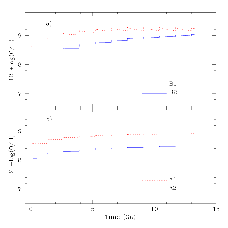
Figure 3: Time evolution of the oxygen abundance, given as $12+log(O/H)$, for the 4 kinds of computed models: a) models of type B burst modes) and b) models of type A attenuated models) with dotted lines corresponding to models of type 1 and solid lines corresponding to models of type 2. The dashed lines limit the range of data taken from Terlevich et al. (1991) and Hoyos & Díaz (2006).

Abundance ratios also give information about the star formation process, essentially the time scale or duration of the bursts, when the production of the elements involved takes place in stars in different mass ranges. This is the case for the N/O ratio. Oxygen is very quickly ejected by the most massive stars. Nitrogen, however, may be created in stars of all masses. Moreover, the production of nitrogen may take place in two ways: 1) the main process requires another element like carbon or oxygen, to synthesize N through the CNO cycle, thus N shows, at least in part, a secondary behavior. In that case the N abundance has to be proportional to the initial abundance of heavy elements and hence the N/O ratio grows with metallicity. There is, however, a proportion of Nitrogen which must have a primary origin, as suggested by the data in Fig. 4 (Izotov & Thuan, 1999; Izotov et al., 2005, 2006) shown by (green) dots which exhibit a constant N/O ratio. Nitrogen may be produced by low and intermediate mass stars (Gavilán et al., 2006) and therefore its contribution may appear in the ISM a certain time after the massive stars have died. In fact, N grows more slowly than the oxygen abundance in the range $7.6<12+log(O/H)<8.2$, which may be explained by this primary behavior (see Mollá et al., 2006, for details). In Fig. 4 we can see the oscillating behavior of the N/O ratio shown by our computed models due to the successive bursts of star formation followed by quiescent periods. At the beginning of a given burst, the N/O ratio decreases, as the O is created and ejected by the most massive stars in the burst; then it increases during the quiescent periods between bursts as the low and intermediate mass stars die and eject their synthesized nitrogen while the oxygen abundance remains constant.

According to the results of this section, model A2 is the one better reproducing the observations, since the total mass, the gas fraction, the star formation rate and the oxygen abundances are within the range shown by data. Therefore, from now onwards, in what regards the ionizing continuum and emission line properties only the A2 model will be analyzed.

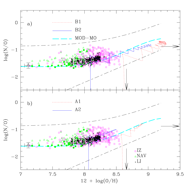
Figure 4: The logarithmic N/O ratio as a function of the oxygen abundance, given as $12+log(O/H)$, for our 4 kinds of computed models: a) type B models; b) type A models. The (black) dashed lines limit the range of data shown by extragalactic Hii regions. The (green) dots and (magenta) squares correspond to the derived values for low metallicity galaxies from Izotov & Thuan (1999); Izotov et al. (2005, 2006); Hoyos & Díaz (2006); Liang et al. (2006); Nava et al. (2006), while the large triangle is the value for the lowest metallicity galaxy in the sample SBS 0335-052W. The long dashed (cyan) lines represents the averaged trend shown by chemical evolution models from Mollá et al. (2006) for spiral and irregular galaxies with continuous star formation. The arrows mark the solar values.

3.2 Evolutionary stellar population synthesis

The convolution of the results of the chemical evolutionary code with the single stellar populations of the synthesis evolutionary code gives us directly the SED, $\rm L_{\lambda}$, in time steps of logt$=$ 0.05.

From this SED the number of hydrogen ionizing photons, coming from hot and young stars of the first spectral types (O-B), can be calculated as:

$$Q(H)=\int_{\nu_{0}}^{\infty}\frac{L_{\nu}}{h\nu}d\nu$$ (11)

where L_ν is the continuum luminosity at frequency $\nu$.

Fig. 5 shows the number of hydrogen ionizing photons as a function of time for model A2. In the first burst, with a total mass of $\sim 30\cdot 10^{6}$ M_⊙ forming stars, the number of massive ionizing stars is high and so it is the number of ionizing photons. The number of ionizing photons per unit stellar mass in our models is ${\log(Q(H)/M_{\odot})}\sim 46.8$ at the starting of the first burst, corresponding to a Zero Age Stellar Population (ZASP) of very low metallicity and then decreases as the cluster ages. This initial number of ionizing photons per unit stellar mass is almost the same for the successive bursts although, decreasing slightly as the abundance increases.

Within each burst the number of ionizing photons decreases by almost two orders of magnitude from 0.5 to 10 Ma, as show in Fig. 6, and by almost 8 orders of magnitude by 100 Ma. Essentially no ionizing photons are available during the quiescent inter-burst periods. At the beginning of each successive burst, the number of ionizing photons raises abruptly but reaching a value progressively lower as less gas is available to form stars. Also, as the mean gas metallicity increases with time, the number of ionizing photons per unit stellar mass decreases (García-Vargas et al., 1995a, b). This effect increases with the age of the ionizing cluster reaching a factor of about 5 at 10 Ma.

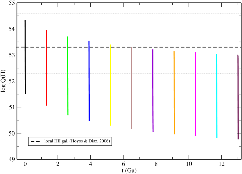
Figure 5: The time evolution of the hydrogen ionizing photons, Q(H), for model A2. The dotted line marks the mode of the distribution for local Hii galaxies found by Hoyos & Díaz (2006). Each coloured line indicates the evolution within a burst. Different colour lines are used for different bursts.

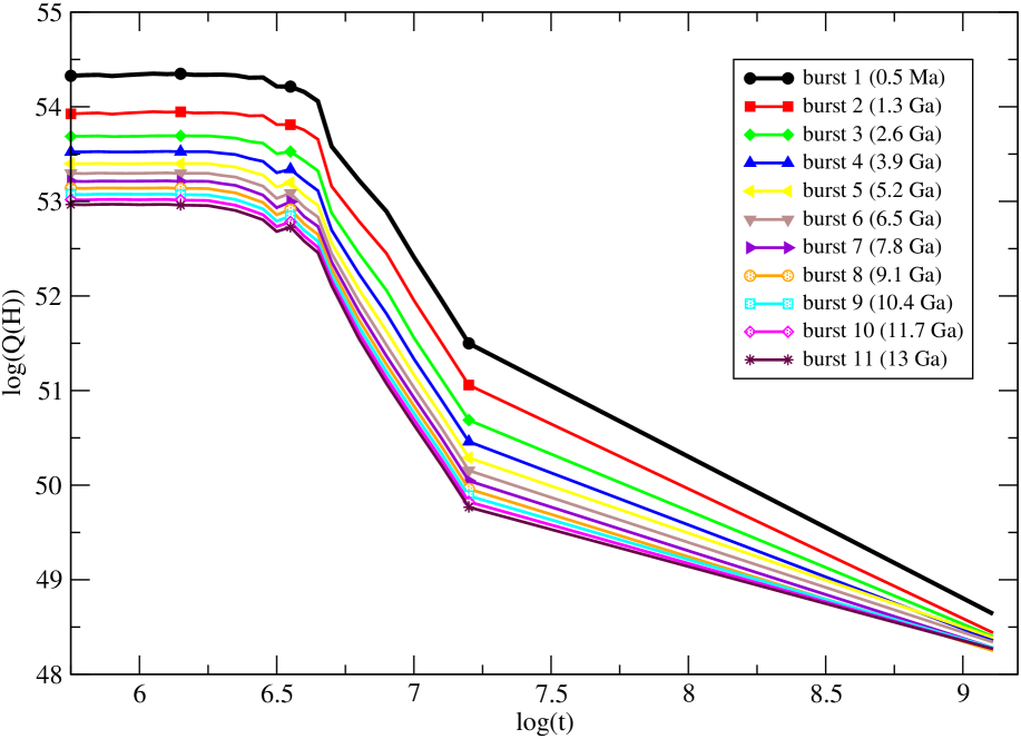
Figure 6: The time evolution of the number of ionizing photons for each of the successive bursts during the 1.3 Ga inter-burst period. The burst number increases downwards. Different colour lines are used for the different bursts.

The average number of ionizing photons observed for local Hii galaxies is $\log{(Q(H))}=53.3$ (Hoyos & Díaz, 2006). This number of ionizing photons, marked as a dotted line in Fig. 5, is reached by model A2 at around the fifth or sixth burst of star formation, that is for the burst occurring 5.2-6.5 Ga after the beginning of the formation of the galaxy, when the predicted star formation rate also fits the data (see Fig. 1). On the other hand, the average derived ionization parameter for the local Hii galaxy sample is $logU=-2.5$ which in our models corresponds to an age of the ionizing population of about 6.5 Ma. It should be noted that during the first 7 Ma of a burst the number of ionizing photons remain essentially constant (see Fig. 6).

Therefore, if the current burst is identified with redshift $z=0$, the formation of the galaxy would have taken place at a redshift $z\sim 0.7$ ( using $H_{0}=74$ km.s¹.Mpc^-1, Macri et al., 2006). Also the observed number of ionizing photons for LCBGs at a redshift $0.46<z<0.7$, estimated as $\log{(Q(H))}\sim 54.6$ (Hammer et al., 2001), would correspond to the value of the first burst of our models. According to these results, our model seems consistent with observations at these intermediate redshifts reproducing at the same time those corresponding to the more luminous local Hii galaxies.

The question of if these galaxies are young galaxies, experiencing their first burst of star formation or if, on the contrary, there exists an underlying population formed some Gas ago, may be addressed by multi-colour photometry. Although a direct detection of the underlying population in LCBG or Hii galaxies is complicated because the observed light is dominated by massive stars, the effect of an underlying stellar population should be easily seen in the observed colours of these galaxies, since any star forming burst previous to the currently observed one will contribute substantially to the total continuum luminosity at the different wavebands.

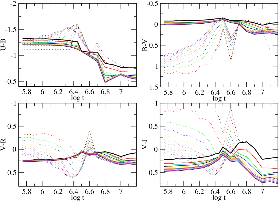
Figure 7: Time evolution of colours for model A2: a) U-B; b) B-V; c) V-R; d) V-I. The meaning of the (coloured) lines for different bursts is the same as in Fig. 5. Solid lines show the pure continuum colours while dotted lines also include the contribution by the strong emission lines.

In Fig. 7 we represent the time evolution of the continuum U-B, B-V, V-R and V-I colours for our model A2 along the first 10 Ma after each burst. The first burst –solid black thick line– follows the expected evolution of a single stellar population of very low metallicity, remaining bluer than during the subsequent bursts where the effect of the accumulated continua from the previous star formation episodes makes colours become redder than expected for a SSP. Even though they are also starbursts in themselves, their star formation efficiency is much lower than that of the first burst, and so is their contribution to the total continuum luminosity which results in redder colours. Furthermore, the metallicity, almost zero for the first burst, increases up to $\rm Z=Z_{\odot}/5$ already during the second burst which also has an reddening effect over the colours.

3.3 Photo-ionization models

The calculated SED in each time step can be used as input ionizing sources in the photo-ionization code to predict the emission lines intensities which provide information about the youngest stellar population which dominates the final spectra.

Fig. 8 shows the relation between the $[OIII]\lambda\lambda$ 4959,5007/H$\beta$ and [OII]$\lambda\lambda$ 3727,3729/H$\beta$ ratios, which constitutes an excitation diagnostics for ionized nebulae. In this diagram, the most excited objects lie up and to the left while the objects with the lowest excitation are at the bottom right.

The data shown in the graph have been extracted mainly from two main sources. First, the compilation from Hoyos & Díaz (2006) which provides emission line measurements, corrected for extinction, published for local Hii galaxies. The sample comprises 450 objects and constitutes a large sample of local Hii galaxies with good-quality spectroscopic data. The sample is rather inhomogeneous in nature, since the data proceed from different instrumental setups, observing conditions and reduction procedures, but have been analysed in a uniform way. Data for these sample objects include the emission line intensities of: [OII]$\lambda\lambda$ 3727,29 Å , [OIII]$\lambda\lambda$ 4959,5007 Å , and [NII]$\lambda\lambda$ 6548,84 Å , all of them relative to H$\beta$, and the equivalent widths of the [OII] and [OIII] emission lines – EW([OII]) EW([OIII]) –, and the H$\beta$ line, EW(H$\beta$). As a second source, we have used the metal poor galaxy data from the Data Release 3 of Sloan Digital Sky Survey, taken from Izotov et al. (2006). The Sloan Digital Sky Survey York et al. (2000) constitutes a large data base of galaxies with well defined selection criteria and observed in a homogeneous way. The SDSS DR3 Abazajian et al. (2005) provides spectra in the wavelength range from 3800 to 9300 Å for $\sim$ 530000 galaxies, quasars and stars. Izotov et al. (2006) extracted $\sim$ 2700 spectra of non-active galaxies with the [OIII]$\lambda$4363 Å emission detected above 1$\sigma$ level. This initial sample was further restricted to the objects with an observed flux in the H$\beta$ emission line larger than $10^{-14}ergs^{-1}cm^{-2}$ and for which accurate abundances could be derived. They have also excluded all galaxies with both [OIII]$\lambda$4959/H$\beta$ $<$ 0.7 and [OII]$\lambda$3727/H$\beta$ $>$ 1.0. Applying all these selection criteria, they obtain a sample of $\sim$ 310 SDSS objects. Data for these sample objects include the emission line intensities of: [OIII]$\lambda$4959,5007 Å and [NII]$\lambda$6584 relative to H$\beta$ and the equivalent width of H$\beta$. They also include the intensity of the [OII] $\lambda\lambda$ 3727,29 Å emission line for the lowest redshift objects.

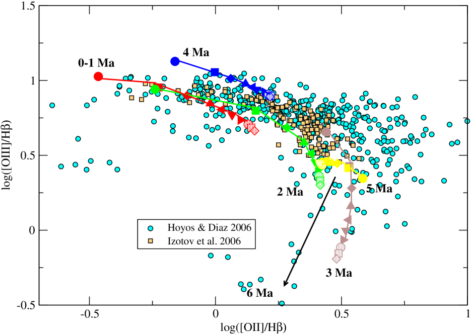
Figure 8: The relation between the oxygen line ratios for model A2. Solid coloured lines join the values reached at the same age by each different burst. Red, green, brown, blue and yellow colours correspond to ages 0-1, 2, 3, 4 and 5 Ma respectively.Different bursts, except the first one, are represented by different symbols: solid circles, squares, diamonds, triangles up, triangles left, triangles down and triangles right correspond to bursts at 1.3, 2.6, 3.9, 5.2, 6.5, 7.8 and 9.1 Ga respectively. Open circles, squares and diamonds correspond to bursts at 10.4, 11.7 and 13.2 Ga respectively. The data are from references cited in the text.

The very young stellar population during the first Ma after each burst produces a high ionization, so the [OIII]/H$\beta$ ratio is high, then it decreases raising again at 4 Ma due to the presence of Wolf Rayet stars that produces a harder continuum (García-Vargas et al., 1995a, 1998). After 5 Ma, the burst evolves to lower values of $log[OIII]/H\beta$. Diagonal lines in this plot correspond to nearly constant ionization parameter and are swept along by the different successive bursts of a given age. High excitation objects, with high $log[OIII]/H\beta$ and low $log[OII]/H\beta$ ratios, have low metallicities and they are not reproduced by our model, which fits better the high metallicity sample, in the middle to right side of the panel.

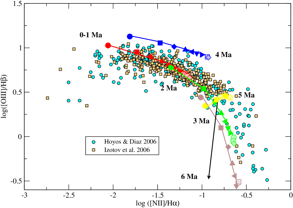
Figure 9: The relation between the excitation parameter, $log([OIII]/H\beta)$, and the metallicity indicator $log([NII]/H\alpha)$ for model A2. The meaning of colours, symbols and lines is the same as in the previous figure.

It can be better seen in Fig.  9, which shows the relation between the excitation parameter, $log([OIII]/H\beta)$, and the metallicity indicator $log([NII]/H\alpha)$ which gives information about the younger populations plus the star formation rate (Kennicutt et al., 1994). At the beginning of the evolution, as we saw in previous sections, the star formation rate is high, and the H$\alpha$ emission of our model is strong. As the galaxy evolves, the H$\alpha$ emission decreases while the [NII] emission increases due to the growth of metallicity.

Our models reproduce the general trend shown by data but cannot reproduce the lower metallicity (low $[NII]/H_{\alpha}$ ratio) objects to the left of the graph. This is due to the fact that the efficiency of the first burst, 33.1 per cent, produces a metallicity which is already too high. A lower efficiency is therefore required to reproduce the observations of the less metallic objects.

3.4 Combined continuum and emission line colours

Once the continuum spectral energy distributions and the different emission line fluxes are computed, we can calculate the contribution of these emission lines to the different broad band filters and then synthesize the colours of our model galaxies. These are the colours which are readily observable through integrated photometry.

We have done so taking into account only the strongest emission lines that contribute to the colour in each broad-band spectral interval at redshift zero. These are: [OII] $\lambda\lambda$ 3727, 3729 Å in U, H$\beta$ $\lambda$ 4861 Å in B, [OIII]$\lambda\lambda$ 4959, 5007 Å in V, H$\alpha$ $\lambda$ 6563 Å in R and [SIII] $\lambda\lambda$ 9069, 9532 Å in I.

The continuum colours and the colours including the emission line contribution at redshift zero are given in columns 3 to 10 of Table 1 for each of the models characterized by their burst number and age (columns 1 and 2). Columns 11 to 15 of the same table give the contribution, in percentage, by the emission lines to the different continuum fluxes.

The necessary information to calculate these contributions for any other redshifts in the nearby universe (z $\lesssim$0.1), is given in Table 2 which lists for each of the models characterized by their burst number and age (columns 1 and 2), the continuum fluxes in each of the U,B,V,R and I (columns 3 to 7) and the fluxes in the [OII], H$\beta$, [OIII], H$\alpha$ and [SIII] lines (columns 8 to 12).

Figure  7 shows, with dotted lines, the new computed colours including the contribution by the different emission lines. As it can be seen the colours do not change by a large amount in the case of U-B or V-R. However the effect in the B-V and V-I colours is rather dramatic. Figure 10 shows the B-V vs V-I colour-colour diagram for model A2. Light blue circles show the continuum colours (solid lines in Figure 7) while black solid ones show the colours computed including the contribution by the stronger emission lines given in Table 1. The inclusion of the contribution by the emission lines to the continuum colours shifts the position of the model points almost perpendicularly to the originally computed ones. The location of blue points is mainly determined, even at zero redshift, by the contribution of strong [OIII]4959,5007 emission lines to the V band. In the same diagram we show the data by Cairós et al. (2001a, b) on BCG as red squares with error bars. These correspond to readily observed colours therefore including both continuum and line emission. No reddening correction has been applied. It can be seen that some of the data are impossible to reproduce by the models which do not take into account the contribution by emission lines, even if some amount of reddening is invoked (the arrow in the diagram shows the correction corresponding to 1 mg visual extinction), while a certain amount of reddening would bring most of the data in agreement with the models. On he other hand the data by Cairós et al. (2002) of resolved locations in Mrk 370, shown in the figure as green triangles, correspond to data that have been corrected for the contribution by emission lines and therefore correspond to pure continuum colours. In these case, the agreement with the models is excellent.

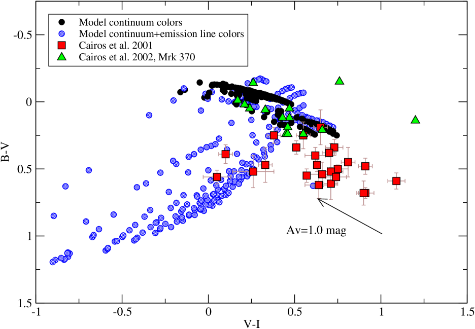
Figure 10: B-V vs V-I colour-colour diagram for model A2. Light blue circles show the continuum colours (solid lines in Figure 7) while black solid ones show the colours computed including the contribution by the stronger emission lines. The data by Cairós et al. (2001a) on BCG and Cairós et al. (2002) in Mrk 370 are included as red squares and green triangles respectively.

4 Discussion

The evolution of Hii galaxies must be considered by looking simultaneously at both continuum and emission line properties, the first one providing information on a long time scale evolution, of the order of Ga, and the second one being related to the evolution in a much shorter time scale, of the order of Ma.

Dottori (1981) suggested the use of the equivalent width of H$\beta$, EW(H$\beta$), as an age estimator for Hii regions, and applied this method to rank the ages of Hii regions in the Magellanic Clouds. If a SSP is considered, the H$\beta$ emission is very high at the beginning of the burst, while the continuum at H$\beta$, dominated by the most massive and luminous stars, is low hence producing a large value of EW(H$\beta$). As the burst evolves, the H$\beta$ luminosity decreases as does the number of ionizing photons, and the contribution to the continuum increases thus lowering the value of EW(H$\beta$). This case corresponds to the thick (black) line in Fig. 11.

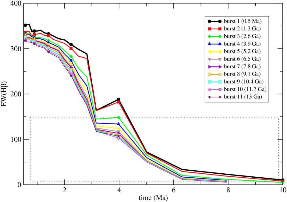
Figure 11: Time evolution of the H$\beta$ equivalent width of model A2. The thick line corresponds to the first star burst of our model, a SSP with very low metallicity. Thin lines represent the successive bursts with same colours as in Fig. 5.

The evolution of the equivalent width in our model is shown in Fig. 11. It is seen that the first burst, that corresponds to a SSP, has an initial equivalent width slightly greater than the successive bursts, which decreases with time reaching very low values ($<$ 40 Å ) 6 Ma after the beginning. When a new burst takes place, new massive ionizing stars form and the EW(H$\beta$) goes up again, although not as much as in the previous one due to the decreasing gas mass involved in the burst, increased metallicity and the accumulated contribution from the continua from the previous bursts. At any rate, even taking into account this contribution, the EW(H$\beta$) remains a good age indicator for the age of the current burst, inside 10 Ma. On the other hand it is not possible to detect the presence of the underlying stellar populations for a given galaxy solely on the basis of this parameter.

The distribution of the EW(H$\beta$) in Hii galaxies shows that most of them have values lower than 150 Å (Terlevich et al., 1991; Hoyos & Díaz, 2006) which, in our models, corresponds to ages greater than 3-4 Ma. (Terlevich et al.2004), from the application of inversion methods, have shown that, globally, this distribution is inconsistent with what is expected from a single burst scenario and resembles more the distribution obtained for a succession of short bursts separated by quiescent periods with little or no star formation.

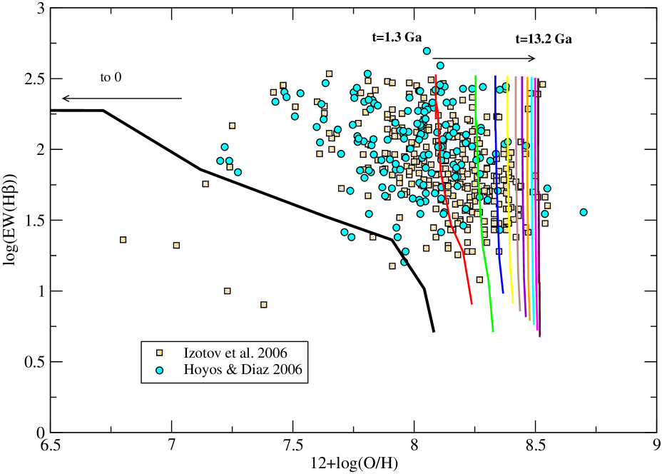
Figure 12: EW(H$\beta$) as a function of the metallicity $12+log(O/H)$ for the model A2. Colours have the same meaning than in Fig. 7. The first burst (solid black line) does not appear in the graph because its abundance is still the primordial one, $12+log(O/H)<<7$.

These results are not that strong when samples showing a restricted metallicity range are analyzed. However, as we have seen before, metallicity increases with time in a way which constrains the SFH which is best reproduced by our A2 model. Fig. 12 shows the evolution of the $\rm EW(H\beta)$ with oxygen abundance. During the duration of the first burst the $\rm EW(H\beta)$ decreases while the oxygen abundance increases from zero to $12+log(O/H)\sim 8$. The successive bursts start with this higher abundance and each of them evolves vertically in a 10 Ma time scale with the $\rm EW(H\beta)$ decreasing rapidly at almost constant oxygen abundance. This occurs because the oxygen is produced by the most massive stars in a very short time and therefore its abundance changes very little during the next 10 Ma after each burst (see Fig. 3). It is clear that our model is able to reproduce the most metallic galaxies in the samples taken from Hoyos & Díaz (2006) and Izotov et al. (2006) where this high abundance is explained as the consequence of the gas being processed by one or more previous generations of stars. An alternative scenario to produce such high oxygen abundances would be the occurrence of a very intense initial star formation burst, with a SFR of the order of 100 M_⊙ Ma^-1, out of the range observed in local Hii galaxies (see Figures 3 and 1). On the other hand, galaxies $12+log(O/H)\leq 8$ are not reproduced by our model. In order to fit these data, a model with a star formation efficiency lower than assumed, that is, $<$ 33 per cent, should be used.

The most informative data to uncover the presence of underlying populations in Hii galaxies consist of the combination of a line emission parameter, which characterizes the properties of the current burst of star formation, and a continuum colour which represents better the SFH in a longer time scale. Fig. 13, left panel, shows the equivalent width of H$\beta$ vs the U-V colour along the evolution of the galaxy for the successive stellar bursts. When a given burst occurs the EW(H$\beta$) is high and decreases as the stellar population ages. We have over-plotted the results for the SSPs from the model Starburst99 (Leitherer et al., 1999, SB99) with two different metallicities as labelled. As expected, our results agree better with the higher metallicity SB99 model. The black line in the left panel, that represents a metal-poor SSP, is too blue compared with the data for a given EW(H$\beta$). In order to decrease EW(H$\beta$) and move the model colour to the red, a more metal-rich SSP was selected (dotted line at the left panel), but even such unrealistic high abundance does not reproduce the observations, as we have shown in Fig. 3. Therefore, the observed trend can not be explained as an age effect since EW(H$\beta$) for low metallicity SSP does not reach values lower than 100Å and does not reproduces the colors, neither as a metallicity effect because such high abundances are not observed in Hii galaxies. It is therefore necessary to include both effects simultaneously, as we have done, to see how the effect of an underlying older population contributing to the color of the continuum makes it redder. From the observational point of view, U-V colours for Hii galaxies are scarce, therefore we have compared our results with those from Hoyos & Díaz (2006) that include galaxies taken from Terlevich et al. (1991) and Salzer et al. (1995) providing the equivalent widths of both the [OII] and [OIII] lines. We have then computed pseudo-colours from the intensities of the adjacent continua of [OII]$\lambda$3727 and [OIII]$\lambda$5007 lines as:

$$EW_{[OII]\lambda 3727}(\rm\AA)=\frac{[OII]\lambda 3727(ergs^{-1})}{I_{cont}(3730)(ergs^{-1}{\AA}^{-1})}$$ (12)

and

$$EW_{[OIII]\lambda 5007}(\rm\AA)=\frac{[OIII]\lambda 5007(ergs^{-1})}{I_{cont}(5010)(ergs^{-1}{\AA}^{-1})}$$ (13)

$$log\left(\frac{I_{cont}(3730)}{I_{cont}(5010)}\right)=log\left(\frac{[OII]\lambda 3727}{[OIII]\lambda 5007}\frac{EW_{[OIII]\lambda 5007}}{EW_{[OII]\lambda 3727}}\right)$$ (14)

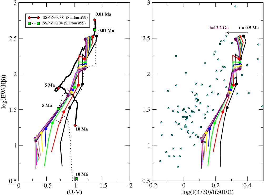
Figure 13: Left panel: The equivalent width of H$\beta$ as a function of the continuum colour for model A2. The results for the SSPs from the model Starburst99 Leitherer et al. (1999) with two different metallicities as labelled are overplotted. Colours have the same meaning as in Fig. 7. Right panel: The equivalent width of H$\beta$ as a function of the pseudo-colour defined by equations 13 to 15 for model A2. The data are from Terlevich et al. (1991) and Salzer et al. (1995). In both panels the large dots mark ages separated 2 Ma.

The right panel of Fig. 13 shows the equivalent width of H$\beta$ as a function of the pseudo-colour defined above for model A2 together with the observational data. It should be noted that no correction for extinction associated with the continuum light has been made. This correction amounts to about 0.15 dex for a standard reddening law and therefore a SSP would always be unable to reproduce the observed colours. Yet our Model A2 produce UV continuum colours which are too blue as compared with the bulk of the observations which indicates that our assumed degree of attenuation is too low.

5 Summary an conclusions

We have explored the viability of a kind of a theoretical model in order to understand how the star formation takes place in Hii galaxies. Our work involves the combination of three different tools: a chemical evolution code, an evolutionary synthesis code and a photo-ionization code, in a self-consistent way, i. e. taking the same assumptions about stellar evolution and nucleosynthesis, and takes into account the resulting metallicity in every time step. The chemical evolution code provides the star formation history of the galaxies as well as the time evolution of the abundances in their interstellar medium, that can be confronted with observations. The evolutionary synthesis code provides the spectrophotometric evolution of the integrated stellar population. Finally, the photo-ionization code uses the properties of the ionizing stellar population to calculated the emission line spectra of the ionized gas.

Each galaxy is modelled assuming an initial amount of unprocessed gas of 10⁸ M_⊙ in a 1 kpc diameter. The evolution is computed along a total duration of 13.2 Ga during which 11 successive starbursts, separated by 1.3 Ga, take place . Different types of models have been computed with different starbursting properties: equal and attenuated bursts, and different values of the initial star formation efficiency. The only model which has proved to be able to fit the observational data is model A2, which consists of attenuated bursts with an initial star formation efficiency of 33.1 per cent. This type of model reproduces the star formation rate estimates of local Hii galaxies and the oxygen abundances of the average metallicity objects although fails to account for the most metal deficient ones which would require models with lower star formation efficiencies than assumed.

We have computed the time evolution of the continuum colours with and without the inclusion of the emission lines. It is shown that both nebular continuum and line emission must be taken into account in the photometric studies of the underlying stellar populations of Hii galaxies. The effect of the emission lines are more pronounced in the B-V and V-I colours.

The combination of parameters which characterize the current star formation on a time scale of Ma, such as the equivalent width of H$\beta$, and the SFH over a time scale of Ga, such as broad-band continuum colours, is found to provide an effective means to uncover the presence of underlying stellar populations. The comparison of models and observations show that in most Hii galaxies SSP are unable to reproduce the relatively red colours shown by data with the observed H$\beta$ equivalent width values requiring the contribution of previous stellar generations. Our model, however, produces U-V colours that are too blue when compared with observations, therefore implying that the successive bursts that take place in Hii galaxies should be even more attenuated than has been assumed in our work.

Table 1: Evolution of continuum and total broad band colors for different bursts along the time after each stellar burst occurs. Only the last burst evolution is shown. The whole table is available in electronic format.

NB	log$\frac{t}{a}$	(U-B)c	(B-V)c	(V-R)c	(V-I)c	(U-B)	(B-V)	(V-R)	(V-I)	% U	% B	% V	% R	% I
11	5.75	-1.205	0.019	0.271	0.480	-1.292	0.748	0.109	0.064	21.254	14.681	57.230	50.400	37.264
11	5.80	-1.202	0.015	0.267	0.474	-1.300	0.694	0.147	0.102	21.845	14.497	54.820	49.812	36.728
11	5.85	-1.203	0.014	0.267	0.472	-1.301	0.706	0.142	-0.065	21.900	14.506	55.610	50.230	42.959
11	5.90	-1.203	0.012	0.264	0.468	-1.311	0.678	0.164	0.117	22.634	14.424	54.460	50.115	37.121
11	5.95	-1.200	0.008	0.260	0.461	-1.345	0.611	0.222	0.177	25.040	14.260	51.674	50.000	37.274
11	6.00	-1.198	0.004	0.255	0.453	-1.378	0.555	0.269	0.225	27.207	13.997	49.152	49.839	37.295
11	6.05	-1.197	0.001	0.252	0.448	-1.383	0.535	0.281	0.236	27.391	13.889	48.246	49.628	37.110
11	6.10	-1.196	-0.002	0.248	0.441	-1.397	0.500	0.307	0.260	28.277	13.716	46.603	49.456	36.942
11	6.15	-1.191	-0.009	0.238	0.426	-1.435	0.407	0.374	0.327	30.679	13.226	41.893	48.686	36.373
11	6.20	-1.189	-0.015	0.232	0.414	-1.457	0.355	0.412	0.363	31.957	12.892	39.095	48.422	36.106
11	6.25	-1.185	-0.021	0.224	0.401	-1.477	0.300	0.452	0.399	33.171	12.523	36.012	48.132	35.917
11	6.30	-1.172	-0.035	0.202	0.367	-1.517	0.136-	0.554	0.504	35.548	11.422	25.592	46.160	34.394
11	6.35	-1.160	-0.047	0.182	0.335	-1.515	0.027-	0.601	0.551	35.367	10.370	17.718	44.104	32.609
11	6.40	-1.138	-0.067	0.148	0.278	-1.475	-0.068-	0.608	0.551	33.098	8.712	9.986	41.101	30.006
11	6.45	-1.113	-0.083	0.116	0.226	-1.403	-0.107-	0.543	0.483	29.051	7.251	6.539	36.974	26.347
11	6.50	-1.073	-0.107	0.061	0.128	-1.274	-0.152-	0.407	0.336	20.862	4.735	2.161	28.889	19.217
11	6.60	-1.020	-0.076	0.084	0.182	-1.079	0.316-	0.000	0.041	12.736	4.400	32.054	24.293	16.869
11	6.70	-0.878	-0.006	0.119	0.277	-0.976	0.024-	0.196	0.272	10.700	2.135	6.592	13.066	6.218
11	6.80	-0.484	0.174	0.206	0.446	-0.497	0.140	0.238	0.447	1.707	0.518	0.000	2.901	0.239
11	6.90	-0.553	0.244	0.291	0.617	-0.553	0.212	0.304	0.617	0.295	0.265	0.000	1.341	0.018
11	7.00	-0.630	0.219	0.331	0.723	-0.628	0.190	0.339	0.723	0.029	0.146	0.000	0.706	0.001
11	7.10	-0.567	0.210	0.152	0.698	-0.567	0.182	0.314	0.698	0.000	0.059	0.00	0.00	0.00

Table 2: Evolution of broad band and the strongest emission lines luminosities along the time after each stellar burst occurs. Only the last burst evolution is shown. The whole table is available in electronic format.

NB	log $\frac{t}{a}$	LU	LB	LV	LR	LI	L([OII])	L(H$\beta$)	L([OIII])	L(H$\alpha$)	L([SIII])
		1040 erg s-1
11	5.75	1.559E+01	1.423E+01	7.080E+00	1.123E+01	7.442E+00	4.252E+00	2.474E+00	9.574E+00	1.1533E+01	4.466E+00
11	5.80	1.569E+01	1.435E+01	7.126E+00	1.126E+01	7.442E+00	4.431E+00	2.458E+00	8.812E+40	1.1296E+01	4.364E+00
11	5.85	1.582E+01	1.447E+01	7.172E+00	1.134E+01	7.483E+00	4.483E+00	2.480E+00	9.080E+00	1.1560E+01	4.459E+00
11	5.90	1.595E+01	1.460E+01	7.225E+00	1.139E+01	7.510E+00	4.716E+00	2.487E+00	8.731E+00	1.1560E+01	4.480E+00
11	5.95	1.612E+01	1.478E+01	7.286E+00	1.144E+01	7.524E+00	5.439E+00	2.483E+00	7.872E+00	1.1560E+01	4.518E+00
11	6.00	1.631E+01	1.500E+01	7.367E+00	1.151E+01	7.552E+00	6.160E+00	2.466E+00	7.196E+00	1.1560E+01	4.538E+00
11	6.05	1.654E+01	1.519E+01	7.448E+00	1.161E+01	7.601E+00	6.303E+00	2.476E+00	7.016E+00	1.1560E+01	4.532E+00
11	6.10	1.680E+01	1.545E+01	7.545E+00	1.172E+01	7.650E+00	6.692E+00	2.481E+00	6.654E+00	1.1586E+01	4.528E+00
11	6.15	1.714E+01	1.584E+01	7.685E+00	1.184E+01	7.685E+00	7.666E+00	2.439E+00	5.598E+00	1.1349E+01	4.439E+00
11	6.20	1.751E+01	1.622E+01	7.835E+00	1.199E+01	7.756E+00	8.309E+00	2.425E+00	5.082E+00	1.1375E+01	4.429E+00
11	6.25	1.792E+01	1.666E+01	8.003E+00	1.216E+01	7.821E+00	8.986E+00	2.410E+00	4.551E+00	1.1401E+01	4.429E+00
11	6.30	1.856E+01	1.746E+01	8.281E+00	1.234E+01	7.850E+00	1.034E+01	2.275E+00	2.878E+00	1.0689E+01	4.158E+00
11	6.35	1.927E+01	1.833E+01	8.599E+00	1.257E+01	7.908E+00	1.065E+01	2.143E+00	1.871E+00	1.0021E+01	3.866E+00
11	6.40	2.050E+01	1.990E+01	9.172E+00	1.299E+01	8.003E+00	1.024E+01	1.919E+00	1.028E+00	9.1614E+00	3.467E+00
11	6.45	2.172E+01	2.158E+01	9.810E+00	1.349E+01	8.152E+00	8.986E+00	1.704E+00	6.936E-01	7.9977E+00	2.946E+00
11	6.50	2.478E+01	2.554E+01	1.136E+01	1.485E+01	8.631E+00	6.600E+00	1.282E+00	2.535E-01	6.0948E+00	2.074E+00
11	6.60	1.929E+01	2.088E+01	9.543E+00	1.273E+01	7.615E+00	2.165E+00	7.670E-01	3.724E+00	3.4910E+00	1.375E+00
11	6.70	1.260E+01	1.556E+01	7.566E+00	1.043E+01	6.596E+00	1.526E+00	3.431E-01	5.396E-01	1.5847E+00	4.419E-01
11	6.80	1.012E+01	1.795E+01	1.023E+01	1.528E+01	1.041E+01	1.776E-01	9.445E-02	0.000E+00	4.6128E-01	2.525E-02
11	6.90	7.074E+00	1.177E+01	7.146E+00	1.154E+01	8.520E+00	2.121E-02	3.171E-02	0.000E+00	1.5847E-01	1.615E-03
11	7.00	5.045E+00	7.821E+00	4.648E+00	7.799E+00	6.110E+00	1.491E-03	1.159E-02	0.000E+00	5.6100E-02	8.127E-05
11	7.10	4.390E+00	7.205E+00	4.247E+00	7.009E+00	5.456E+00	6.406E-08	4.361E-03	0.000E+00	2.0891E-05	0.000E+00

References

- Abazajian et al. (2005) Abazajian K. et. al., 2005, AJ, 129, 1755
- Aller (1984) Aller L. H., 1984, Physics of thermal gaseous nebulae Dordrecht, D. Reidel Publishing Co. (Astrophysics and Space Science Library. Volume 112)
- Asplund et al. (2005) Asplund M., Grevesse N., Sauval A. J., 2005, in ASP Conf. Ser. 336: Cosmic Abundances as Records of Stellar Evolution and Nucleosynthesis, p. 25
- Bertelli et al. (1994) Bertelli G., Bressan A., Chiosi C., Fagotto F., Nasi E., 1994, A&AS, 106, 275
- Bradamante et al. (1998) Bradamante F., Matteucci F., D’Ercole A., 1998, A&A, 337, 338
- Bressan et al. (1993) Bressan A., Fagotto F., Bertelli G., Chiosi C., 1993, A&AS, 100, 647
- Cairós et al. (2003) Cairós L. M., García-Lorenzo B., Caon N., Vílchez J. M., Papaderos P., Noeske K., 2003, Ap&SS, 284, 611
- Cairós et al. (2002) Cairós L. M., Caon N., García-Lorenzo B., Vílchez J. M., Muñoz-Tuñón C., 2002, ApJ, 577, 164
- Cairós et al. (2001b) Cairós L. M., Caon N., Vílchez J. M., González-Pérez J. N., Muñoz-Tuñón C., 2001, ApJS, 136, 393
- Cairós et al. (2001a) Cairós L. M., Vílchez J. M., González Pérez J. N., Iglesias-Páramo J., Caon N., 2001, ApJS, 133, 321
- Carigi et al. ( 2002) Carigi L., Hernandez X., Gilmore G., 2002, MNRAS, 334, 117
- Chabrier (2003) Chabrier G., 2003, ApJL, 586, L133
- Clegg & Middlemass (1987) Clegg R. E. S., Middlemass D., 1987, MNRAS, 228, 759
- Dottori (1981) Dottori H. A., 1981, Ap.& Space Sience, 80, 267
- Fagotto et al. (1994) Fagotto, F. and Bressan, A. and Bertelli, G. and Chiosi, C.,1994,A&AS, 104,365F
- Fagotto et al. (1994) Fagotto, F. and Bressan, A. and Bertelli, G. and Chiosi, C.,1994,A&AS, 105,29F
- Fagotto et al. (1994) Fagotto, F. and Bressan, A. and Bertelli, G. and Chiosi, C.,1994,A&AS, 105,39F
- Ferland (1980) Ferland G. J., 1980, PASP, 92, 596
- Ferland et al. (1998) Ferland G. J., Korista K. T., Verner D. A., Ferguson J. W., Kingdon J. B., Verner E. M., 1998, PASP, 110, 761
- Ferrini et al. (1992) Ferrini F., Matteucci F., Pardi C., Penco U., 1992, ApJ, 387, 138
- Ferrini et al. (1994) Ferrini F., Mollá M., Pardi M. C., Díaz A. I., 1994, ApJ, 427, 745
- Ferrini et al. (1990) Ferrini F., Penco U., Palla F., 1990, A&A, 231, 391
- Galli et al. (1995) Galli D., Palla F., Ferrini F., Penco U., 1995, ApJ, 443, 536
- García-Vargas et al. (1995a) García-Vargas M. L., Bressan A., Díaz A. I., 1995, A&AS, 112, 35
- García-Vargas et al. (1995b) García-Vargas M. L., Bressan A., Díaz A. I., 1995, A&AS, 112, 13
- García-Vargas et al. (1998) García-Vargas M. L., Mollá M., Bressan A., 1998, A&AS, 130, 513
- Garnett et al. (1999) Garnett D. R., Shields G. A., Peimbert M., Torres-Peimbert S., Skillman E. D., Dufour R. J., Terlevich E., Terlevich R. J., 1999, ApJ, 513, 168
- Gavilán et al. (2005) Gavilán M., Buell J. F., Mollá M., 2005, A&A, 432, 861
- Gavilán et al. (2006) Gavilán M., Mollá M., Buell J. F., 2006, A&A, 450, 509
- Hammer et al. (2001) Hammer F., Gruel N., Thuan T. X., Flores H., Infante L., 2001, ApJ, 550, 570
- Henry et al. (2000) Henry R. B. C., Edmunds M. G., Köppen J., 2000, ApJ, 541, 660
- Hoyos & Díaz (2006) Hoyos C., Díaz A. I., 2006, MNRAS, 365, 454
- Hoyos et al. (2004) Hoyos C., Guzmán R., Bershady M. A., Koo D. C., Díaz A. I., 2004, AJ, 128, 1541
- Iwamoto et al. (1999) Iwamoto K., Brachwitz F., Nomoto K., Kishimoto N., Umeda H., Hix W. R., Thielemann F., 1999, ApJS, 125, 439
- Izotov & Thuan (2004) Izotov Y. I., Thuan T. X., 2004, ApJ, 616, 781I
- Izotov et al. (2006) Izotov Y. I., Stasińska G., Meynet G., Guseva N. G., Thuan T. X., 2006, A&A, 448, 955
- Izotov & Thuan (1999) Izotov Y. I., Thuan T. X., 1999, ApJ, 511, 639
- Izotov et al. (2005) Izotov Y. I., Thuan T. X., Guseva N. G., 2005, ApJ
- Kennicutt et al. (1994) Kennicutt Jr. R. C., Tamblyn P., Congdon C. E., 1994, ApJ, 435, 22
- Kroupa (2001) Kroupa P., 2001, MNRAS, 322, 231
- Larsen et al. (2001) Larsen T. I., Sommer-Larsen J., Pagel B. E. J., 2001, MNRAS, 323, 555
- Legrand (2000) Legrand F., 2000, A&A, 354, 504
- Leitherer et al. (1999) Leitherer C., Schaerer D., Goldader J. D., Delgado R. M. G., Robert C., Kune D. F., de Mello D. F., Devost D., Heckman T. M., 1999, ApJS, 123, 3
- Lejeune et al. (1997) Lejeune T., Cuisinier F., Buser R., 1997, A&A Supl.S., 125, 229
- Liang et al. (2006) Liang Y. C., Yin S. Y., Hammer F., Deng L. C., Flores H., Zhang B., 2006, ApJ, 652, 257
- Macri et al. (2006) Macri L. M., Stanek K. Z., Bersier D., Greenhill L. J., Reid M. J., 2006, ApJ, 652, 1133
- Mas-Hesse & Kunth (1999) Mas-Hesse J. M., Kunth D., 1999, A&A, 349, 765
- Meyer et al. (2000) Meyer M. R., Adams F. C., Hillenbrand L. A., Carpenter J. M., Larson R. B., 2000, Protostars and Planets IV, 121
- Mollá & García-Vargas (2000) Mollá M., García-Vargas M. L., 2000, A&A, 359, 18
- Mollá et al. (2006) Mollá, M., Vílchez J. M., Gavilán M., Díaz A. I., 2006, MNRAS, 372, 1069
- Mollá & Díaz (2005) Mollá, M., Díaz A. I., 2005, MNRAS, 358,521M
- Mouhcine & Contini ( 2002) Mouhcine M., Contini T., 2002, A&A, 389, 106
- (53) Moy E., Rocca-Volmerange B., Fioc M., 2001, A&A, 365, 347
- Nava et al. (2006) Nava A., Casebeer D., Henry R. B. C., Jevremovic D., 2006, ApJ, 645, 1076
- (55) Nomoto K., Thielemann F.-K., Yokoi K., 1984, ApJ, 286, 644
- Portinari et al. ( 1998) Portinari L., Chiosi C., Bressan A., 1998, A&A, 334, 505
- Ruiz-Lapuente et al. (2000) Ruiz-Lapuente P., Blinnikov S., Canal R., Mendez J., Sorokina E., Visco A., Walton N., 2000, Memorie della Societa Astronomica Italiana, 71, 435
- Salzer et al. (1995) Salzer J. J., Moody J. W., Rosenberg J. L., Gregory S. A., Newberry M. V., 1995, AJ, 109, 2376
- Sargent & Searle (1970) Sargent W. L. W., Searle L., 1970, ApJ, 162, L155
- Scalo (1998) Scalo J., 1998, in ASP Conf. Ser. 142: The Stellar Initial Mass Function (38th Herstmonceux Conference), 201
- Scalo (1986) Scalo J. M., 1986, Fundamentals of Cosmic Physics, 11, 1
- Shiet al. (2006) Shi F., Kong X., Cheng F.-Z., 2006, Chinese Journal of Astronomy and Astrophysics, 6, 641
- (63) Stasińska G., Izotov Y., 2003, A&A, 397, 71
- Talbot & Arnett ( 1973) Talbot R. J., Jr., & Arnett W. D., 1973, ApJ, 186, 51
- (65) Taylor C. L., Brinks E., Pogge R. W., Skillman E. D., 1994, AJ, 107, 971
- Telles et al. ( 1997) Telles E., Melnick J., Terlevich R., 1997, MNRAS, 288, 78
- Terlevich et al. (1991) Terlevich R., Melnick J., Masegosa J., Moles M., Copetti M. V. F., 1991, A&A Supl.Series, 91, 285
- (68) Terlevich R., Silich S., Rosa-González D., Terlevich E., 2004, MNRAS, 348, 1191
- Thuan & Izotov (2005) Thuan T. X., Izotov Y. I., 2005, ApJ, 627, 739
- Tolstoy (2003) Tolstoy E., 2003, Ap&SS, 284, 579
- (71) van Zee L., Barton E. J., Skillman E. D., 2004, AJ, 128, 2797
- (72) Vázquez G. A., Carigi L., González J. J., 2003, A&A, 400, 31
- Woosley & Weaver (1995) Woosley S. E., Weaver T. A., 1995, ApJS, 101, 181
- Wyse (1997) Wyse R. F. G., 1997, ApJL, 490, L69
- York et al. (2000) York D. G., et al., 2000, AJ, 120, 1579