Critical behavior of interacting two-polymer system in a fractal solvent: an exact renormalization group approach

Abstract

We study the polymer system consisting of two polymer chains situated in a fractal container that belongs to the three–dimensional Sierpinski Gasket (3D SG) family of fractals. Each 3D SG fractal has four fractal impenetrable 2D surfaces, which are, in fact, 2D SG fractals. The two-polymer system is modelled by two interacting self-avoiding walks (SAWs), one of them representing a 3D floating polymer, while the other corresponds to a chain adhered to one of the four 2D SG boundaries. We assume that the studied system is immersed in a poor solvent inducing the intra-chain interactions. For the inter-chain interactions we propose two models: in the first model (ASAWs) the SAW chains are mutually avoiding, whereas in the second model (CSAWs) chains can cross each other. By applying an exact Renormalization Group (RG) method, we establish the relevant phase diagrams for $b=2,3$ and $b=4$ members of the 3D SG fractal family for the model with avoiding SAWs, and for $b=2$ and $b=3$ fractals for the model with crossing SAWs. Also, at the appropriate transition fixed points we calculate the contact critical exponents, associated with the number of contacts between monomers of different chains. Throughout the paper we compare results obtained for the two models and discuss the impact of the topology of the underlying lattices on emerging phase diagrams.

1 Introduction

The self–avoiding walk (SAW) is well-disposed as a standard lattice model for a flexible linear polymer chain in various types of solvents [1]. In this model, the monomers that comprise a polymer chain are related to the steps of a random walk that must not contain self-intersections, while the surrounding solvent is represented by an underlying lattice. In a good solvent, with each step of the SAW we associate the same weight factor $x$, while in a poor solvent, when two non-consecutive monomers of a polymer chain become nearest neighbors, we introduce the additional statistical factor $u$, which corresponds to the intra-chain energy $\epsilon_{u}<0$. Even though an isolated polymer chain is difficult to observe experimentally, numerous studies of the single-chain statistics have been upheld as a requisite step towards understanding the statistics of many-chain systems. A natural extension of a single polymer concept is a model of two interacting linear polymers, which may be relevant to perceive behavior of multicomponent polymer solutions [2]. To study the critical properties of the two-polymer system we shall apply the following two models: The first is the model of two mutually avoiding self-avoiding walks (ASAWs), whose paths on a lattice cannot cross each other, and the second is the model of two mutually crossing self-avoiding walks (CSAWs), that is, the case of the two SAWs whose paths can intersect each other. Various types of models with two avoiding SAWs have been successfully applied in the studies of phase transition of diblock copolymers [3, 4], as well as in the studies of unzipping double-stranded DNA molecules [5, 6, 7, 8]. On the other hand, the model with two crossing SAWs was applied for studying the collapse transition of two-chain interacting system on three- and four-simplex lattice [9, 10], and Euclidean lattices [11], as well as to study two randomly interacting directed polymers on diamond hierarchical lattice [12, 13].

In this paper we apply both ASAWs and CSAWs model to study the two-polymer system that displays both intra- and inter-chain interactions, on the three-dimensional (3D) fractal lattices, which belong to the Sierpinski gasket (SG) family of fractals. We assume that one of the two polymers is a floating chain in the bulk of a 3D SG fractal, while the other is a polymer chain that stays affixed to one of the four boundary surfaces (being actually 2D SG fractals) [14]. In the ASAWs model we assume that two SAWs are in contact when they approach each other at the distance which is equal to a lattice constant, and in this situation we ascribe the contributing contact energy $\epsilon_{v}$ to the total model energy. Similarly, in the CSAWs model we assume that each crossing between two SAW paths corresponds to a contact of two monomers that belong to different polymer chains, and therefore we associate the contact energy $\epsilon_{c}$ with such a crossing. Since in both models, one of two polymers is adhered to one of the fractal boundary surfaces, and because its monomers take effect of surface interacting points for the bulk floating polymer chain, the proposed models may also be of interest for the problem of surface-interacting polymer chain in homogeneous [15, 16, 17] and disordered media [18].

The main goal of this study is to establish phase diagrams in the space of interaction parameters (which consists of the intra- and inter-chain interaction energy parameters), for both models, as well as to calculate the contact critical exponents that describe behavior of numbers of monomer-monomer contacts between two polymer chains.

This paper is organized as follows. In section 2 of the paper, we first describe the 3D SG fractals for general scaling parameter $b$, as well as the ASAWs model. Then, we present the general framework of an exact renormalization group method, within the model, and elaborate on the phase diagrams, obtained for the fractals designated by $b=2,3$ and $b=4$. We also display our findings for the contact exponents (associated with the number of contacts between the two SAWs). The CSAWs model is described in section 3. Again, by applying an exact RG method, which is in the latter case technically more complicated, phase diagrams and contact exponents for $b=2$ and 3 SG fractals are obtained, and discussed. Brief summary and the concomitant conclusion are presented in section 4. Explicit form of the RG equations for particular fractals are given in appendices.

2 The model of two evading self-avoiding walks

In this section we are going to apply the renormalization group (RG) method to the model of two mutually avoiding self-avoiding walks on the 3D SG family of fractals. First, we give a summary of the basic properties of these fractals. We start with recalling the fact that each member of the 3D SG fractal family is labeled by an integer $b\geq 2$ and can be constructed in stages. At the first stage ($r=1$) of the construction there is a tetrahedron of base $b$ that contains $b(b+1)(b+2)/6$ upward oriented unit tetrahedrons. The subsequent fractal stages are constructed recursively, so that the complete self-similar fractal lattice can be obtained as the result of an infinite iterative process of successive $(r\to r+1)$ enlarging the fractal structure $b$ times, and replacing the smallest parts of enlarged structure with the initial ($r=1$) structure. Fractal dimension $d_{f}$ of the 3D SG fractal is equal to $d_{f}^{3D}={{\ln[{{b(b+1)(b+2)}/6}}]/{\ln b}}$. Each of the four boundaries of the 3D SG fractal is itself a 2D SG fractal, with the fractal dimension $d_{f}^{2D}=\ln[b(b+1)/2]/\ln b\>$.

In the terminology that applies to the SAW, we assign the weight $x_{3}$ to a step of the SAW in the bulk (3D SG fractal), which represents a floating polymer (we mark it by $P_{3}$), and the weight $x_{2}$ to a step of the SAW performed on one of the fractal boundaries (2D SG fractal), which represents a 2D surface-adhered polymer (marked by $P_{2}$), whose monomers act as interacting counterparts for monomers of the 3D polymer chain. To describe the intra-chain interaction of $P_{3}$ chain, we introduce the Boltzmann factor $u=e^{-\epsilon_{u}/k_{B}T}$, where $\epsilon_{u}<0$ is the interaction energy of two non-consecutive neighboring monomers of $P_{3}$.

In ASAWs model the two SAWs, that represent polymer chains, must not intersect each other. We assume that monomers, belonging to different chains, interact when they reach a distance which is equal to a fractal lattice constant, and to a such mutual position of $P_{3}$ and $P_{2}$ monomers we associate the weight factor $v=e^{-\epsilon_{v}/k_{B}T}$ (see figure 1(a)), where $\epsilon_{v}\leq 0$ is the appropriate inter-chain interaction energy.

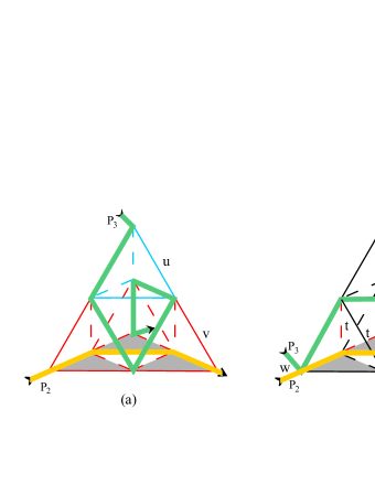
Figure 1: The structure of the three-dimensional SG fractal, for $b=2$, at the first stage of construction, with an example of the bulk polymer chain ($P_{3}$) depicted by green line and the surface-adhered polymer chain ($P_{2}$) depicted by yellow line. The shaded area represents the adhering surface (the two-dimensional SG fractal). The intra-chain interactions $u$, for the $P_{3}$ polymer, are depicted by blue bonds. In the ASAWs model (a) the SAW paths, representing $P_{3}$ and $P_{2}$ polymers, cannot intersect each other, and two SAWs interact when approach each other at a distance which is equal to a lattice constant (red bonds, weighted with $v$). On the other hand, in the case of CSAWs model (b), the polymers $P_{3}$ and $P_{2}$ are cross-linked at the two sites, so that each contact contributes the weight factor $w$, while the red bonds (marked by $t$) correspond to the interactions between those monomers which are nearest neighbors to the cross-linked points. The two depicted examples for ASAWs (a) and CSAWs models (b), contribute the weights $x_{3}^{5}x_{2}^{3}u^{4}v^{12}$ and $x_{3}^{4}x_{2}^{3}w^{2}t^{3}$, respectively.

To describe exactly all possible configurations of the two-chain polymer system within the adopted model, we need four restricted partition functions $A^{(r)}$, $B^{(r)}$, $C^{(r)}$ and $D^{(r)}$, which are defined as

$$A^{(r)}=\sum_{N_{3},L}{\mathcal{A}}^{(r)}(N_{3},L)x_{3}^{N_{3}}u^{L},\quad B^{(r)}=\sum_{N_{3},L}{\mathcal{B}}^{(r)}(N_{3},L)x_{3}^{N_{3}}u^{L},\quad$$

$$C^{(r)}=\sum_{N_{2}}{\mathcal{C}}^{(r)}(N_{2})x_{2}^{N_{2}},\quad D^{(r)}=\sum_{N_{2},N_{3},L,M}{\mathcal{D}}^{(r)}(N_{2},N_{3},L,M)x_{2}^{N_{2}}x_{3}^{N_{3}}u^{L}v^{M},$$ (2.1)

where ${\mathcal{A}}^{(r)}$, ${\mathcal{B}}^{(r)}$, ${\mathcal{C}}^{(r)}$, and ${\mathcal{D}}^{(r)}$ represent the numbers of particular configurations, consisting of one or two SAW strands on the $r$-th fractal structure (see figure 2). For instance, ${\mathcal{D}}^{(r)}(N_{2},N_{3},L,M)$ is the number of configurations consisting of $N_{3}$-step $P_{3}$ chain with $L$ pairs of non-consecutive nearest-neighbor monomers, and $N_{2}$-step $P_{2}$ chain, such that there are $M$ contacts between these two chains. The recursive nature of the fractal construction implies the following recursion relations for restricted partition functions

$$A^{\prime} = \sum_{N_{A},N_{B}}a(N_{A},N_{B})\,A^{N_{A}}B^{N_{B}}\,,$$ (2.2)

$$B^{\prime} = \sum_{N_{A},N_{B}}b(N_{A},N_{B})\,A^{N_{A}}B^{N_{B}}\,,$$ (2.3)

$$C^{\prime} = \sum_{N_{C}}c(N_{C})\,C^{N_{C}}\,,$$ (2.4)

$$D^{\prime} = \sum_{N_{A},N_{B},N_{C},N_{D}}d(N_{A},N_{B},N_{C},N_{D})\,A^{N_{A}}B^{N_{B}}C^{N_{C}}D^{N_{D}}\>,$$ (2.5)

where we have used the prime symbol as a superscripts for $(r+1)$-th restricted partition functions and no indices for the $r$-th order partition functions. These relations can be considered as the RG equations for the problem under study, with the initial conditions

$$A^{(0)}=x_{3}\,,\quad B^{(0)}=x_{3}^{2}u^{4}\,,\quad C^{(0)}=x_{2}\,,\quad\,D^{(0)}=x_{3}x_{2}v^{4}\,,$$ (2.6)

which correspond to the unit tetrahedron.

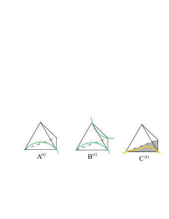
Figure 2: Schematic depiction of restricted generating functions used in the description of all possible two-SAW configurations, within the $r$-th stage of the 3D SG fractal structure, for ASAWs model. The 3D floating chain is depicted by green line, while the 2D surface-adhered chain is depicted by the yellow one. The interior details of the $r$-th stage fractal structure, as well as details of the chains, are not shown (for the chains, they are manifested by the wiggles of the SAW paths). The functions $A^{(r)}$, $B^{(r)}$, and $C^{(r)}$, describe one-polymer configurations (they are the same for both ASAWs and CSAWs models), while the function $D^{(r)}$ depicts the inter-chain configurations of ASAWs model.

Equation (2.4), alone, describes a single SAW on 2D SG fractal, whereas (2.2) and (2.3) are RG equations for a single SAW on 3D SG fractal. Critical properties of the SAW, based on the analysis of these equations, have been well established previously, and here we recall their basic properties relevant for the present work.

First, we describe the behavior of a single 2D SG chain. The RG equation (2.4), for any $b$, has only one non-trivial fixed point $C^{*}$, corresponding to the extended polymer phase [19, 20], that is, the 2D SG chain is always swollen, and it cannot be in the compact phase. The corresponding eigenvalue $\lambda_{\nu_{2}}$ of (2.4) is larger than 1, and determines the value of the critical exponent $\nu_{2}=\ln b/\ln\lambda_{\nu_{2}}$, that governs the behavior of the mean end-to-end distance of 2D SG chain $\langle R\rangle\sim{\langle N_{2}\rangle}^{\nu_{2}}$, where $\langle N_{2}\rangle$ is the average number of 2D SG SAW steps.

In what follows we provide short summary of the results concerning the critical behavior of a solitary 3D SG chain. Depending on the value of the intra-chain interaction parameter $u$, a single 3D SG chain can be found in three phases: extended chain (for $u<u_{\theta}$), $\theta$-chain (when $u=u_{\theta}$) and globule ($u>u_{\theta}$). These phases (for arbitrary $b$) are described by the fixed points $(A_{E},B_{E})$, $(A_{\theta},B_{\theta})$ and $(A_{G},B_{G})$, respectively [21, 22, 23]. The mean end-to-end distance $\langle R\rangle\sim{\langle N_{3}\rangle}^{\nu_{3}}$ of SAW on 3D SG fractal, is equal to $\nu_{3}=\ln b/\ln\lambda_{\nu_{3}}$, where $\lambda_{\nu_{3}}$ is the largest eigenvalue of the linearized RG equations (2.2) and (2.3), at the corresponding fixed point. For each 3D SG fractal, the following relationship $\nu_{3}^{E}>\nu_{3}^{\theta}>\nu_{3}^{G}$, is valid, where $\nu_{3}^{E}$, $\nu_{3}^{\theta}$ and $\nu_{3}^{G}$ are the end-to-end distance critical exponents in extended, $\theta$ and globule phase, respectively.

The interacting configurations of $P_{2}$ and $P_{3}$ chains are described with the restricted partition function $D^{(r)}$. The mean number of contacts between $P_{2}$ and $P_{3}$, on the $r$-th stage of fractal construction, is equal to

$$\langle M^{(r)}\rangle={1\over D^{(r)}}\sum_{N_{2},N_{3},L,M}M{\mathcal{D}}^{(r)}x_{2}^{N_{2}}x_{3}^{N_{3}}u^{L}v^{M}={v\over D^{(r)}}\frac{\partial D^{(r)}}{\partial v}\>.$$ (2.7)

On the other hand, taking into account the function dependance $D^{(r+1)}=D^{(r+1)}(A^{(r)},B^{(r)},C^{(r)},D^{(r)})$, and the fact that $A^{(r)}$, $B^{(r)}$, and $C^{(r)}$ do not depend on the interaction parameter $v$, we have

$$\frac{\partial D^{(r+1)}}{\partial v}=\frac{\partial D^{(r+1)}}{\partial D^{(r)}}\frac{\partial D^{(r)}}{\partial v}\,,$$ (2.8)

from which follows that, in the vicinity of the transition fixed point $(A^{*},B^{*},C^{*},D^{*})$ of the two-polymer system, the mean number of contacts $\langle M^{(r)}\rangle$, for large $r$, behaves as $\langle M^{(r)}\rangle\sim\lambda_{D}^{r}$, where

$$\lambda_{D}={\left(\frac{\partial D^{(r+1)}}{\partial D^{(r)}}\right)}^{*}\>,$$ (2.9)

is relevant eigenvalue of RG equation (2.5), calculated at the transition fixed point. Knowing that $\langle{N_{3}^{(r)}}\rangle\sim\lambda_{\nu_{3}}^{r}$, one obtains $\ln\langle M^{(r)}\rangle/{\ln\langle N_{3}^{(r)}\rangle}\sim{\ln\lambda_{D}}/{\ln\lambda_{\nu_{3}}}$, i.e. the following scaling relation is satisfied

$$\langle M^{(r)}\rangle\sim\langle N_{3}^{(r)}\rangle^{\phi}\>,$$ (2.10)

where

$$\phi=\frac{{\ln\lambda_{D}}}{\ln\lambda_{\nu_{3}}}\,,$$ (2.11)

is so-called contact critical exponent.

To establish the exact forms of RG equations, for each fractal, one needs to find the coefficients $a$, $b$, $c$, and $d$, that appear in (2.2)–(2.5). Using the computer facilities, by direct enumeration and classification of all possible SAW configurations on the first stage of fractal construction, it is feasible to find these coefficients for fractals labelled by $b=2,3$ and 4 (see A). Precise numerical analysis of the obtained RG equations (for $b=2,3$, and 4) reveals that two-polymer system can reside in several phases, depending on the values of the interaction parameters $u$ and $v$. In particular, for each value of $u$, there is a critical value $v=v_{c}(u)$, such that for $v<v_{c}(u)$ the two chains exist almost independently in the solution. This is indicated by the fact that $(A^{*},B^{*})$, and $C^{*}$ retain their fixed values that correspond to the solitary chain on 3D SG, and 2D SG, respectively (see table 1), and confirmed by calculating the mean number of contacts $\langle M^{(r)}\rangle$ between the chains, which quickly approaches some constant value as $r\to\infty$.

Table 1: Coordinates of transition fixed points $(A^{*},B^{*},C^{*},D^{*})$, obtained via renormalization group approach, for ASAWs model on 3D SG fractals labelled by $b=2,3$ and 4. Also, we give the corresponding relevant eigenvalues $\lambda_{\nu_{3}}$ and $\lambda_{D}$, together with the pertaining values of contact critical exponents $\phi$. For all values of $b$ studied, when $v<v_{c}(u)$, eigenvalue $\lambda_{D}$ is not relevant, and the mean number of contacts between the chains is finite (thus the values of $\lambda_{D}$ and $\phi$ are not given for these cases).

$b$ $v$ $A^{*}$ $B^{*}$ $C^{*}$ $D^{*}$ $\lambda_{\nu_{3}}$ $\lambda_{D}$ $\phi$ extended 3D chain $(u<u_{\theta})$ $v<v_{c}(u)$ 0.4294 0.0499 0.6180 0.1165 2.7965 $<1$ – 2 $v=v_{c}(u)$ 0.4294 0.0499 0.6180 2.3303 2.7965 2.0904 0.7170 $v>v_{c}(u)$ 0.4294 0.0499 0 3.0887 2.7965 2.9537 1.0532 $v<v_{c}(u)$ 0.3420 0.0239 0.5511 0.0779 5.3620 $<1$ – 3 $v=v_{c}(u)$ 0.3420 0.0239 0.5511 1.5388 5.3620 2.7879 0.6105 $v>v_{c}(u)$ 0.3420 0.0239 0 2.8591 5.3620 4.6651 0.9171 $v<v_{c}(u)$ 0.2899 0.0122 0.5063 0.0580 8.6911 $<1$ – 4 $v=v_{c}(u)$ 0.2899 0.0122 0.5063 1.2051 8.6911 3.4427 0.5717 $v>v_{c}(u)$ 0.2899 0.0122 0 2.0837 8.6911 8.4170 0.9852 3D $\theta$–chain $(u=u_{\theta})$ $v<v_{c}(u_{\theta})$ 1/3 1/3 0.6180 0.0613 100/27 $<1$ – 2 $v=v_{c}(u_{\theta})$ 1/3 1/3 0.6180 0.6180 100/27 1.8526 0.4709 $v>v_{c}(u_{\theta})$ 1/3 1/3 0 0.8229 100/27 2.4514 0.6848 $v<v_{c}(u_{\theta})$ 0.2071 0.4307 0.5511 0.0211 8.7231 $<1$ – 3 $v=v_{c}(u_{\theta})$ 0.2071 0.4307 0.5511 0.5773 8.7231 2.4203 0.4081 $v>v_{c}(u_{\theta})$ 0.2071 0.4307 0 1.2781 8.7231 3.7800 0.6139 $v<v_{c}(u_{\theta})$ 0.1918 0.3393 0.5063 0.0180 15.424 $<1$ – 4 $v=v_{c}(u_{\theta})$ 0.1918 0.3393 0.5063 0.5758 15.424 3.5367 0.4617 $v>v_{c}(u_{\theta})$ 0.1918 0.3393 0 0.7984 15.424 5.9331 0.6508 3D globule $(u>u_{\theta})$ $v<v_{c}(u)$ 0 $22^{-1/3}$ 0.6180 0 4 $<1$ – 2 $v=v_{c}(u)$ 0 $22^{-1/3}$ 0.6180 0.7637 4 2.4163 0.6364 $v>v_{c}(u)$ 0 $22^{-1/3}$ 0 0.7637 4 2.4163 0.6364 $v<v_{c}(u)$ 0 $\infty$ 0.5511 0 9.772 $<1$ – 3 $v=v_{c}(u)$ 0 $\infty$ 0.5511 $\infty$ 9.772 2 0.3041 $v>v_{c}(u)$ 0 $\infty$ 0 $\infty$ 9.772 2 0.3041 $v<v_{c}(u)$ 0 $22^{-1/3}$ 0.5063 0 16 $<1$ – 4 $v=v_{c}(u)$ 0 $22^{-1/3}$ 0.5063 0.7637 16 5.8387 0.6364 $v>v_{c}(u)$ 0 $22^{-1/3}$ 0 0.7637 16 5.8387 0.6364

For $v=v_{c}(u)$ fixed values $(A^{*},B^{*})$ and $C^{*}$ remain the same as for $v<v_{c}(u)$, but $D^{*}$ becomes larger, and $\langle M^{(r)}\rangle$ increases with $r$, obeying the scaling relation (2.10), with eigenvalue $\lambda_{D}$ being larger than one. Although there are large number of contacts between them, both chains also have large parts that are not interconnected. Even for $v>v_{c}(u)$ fixed value $(A^{*},B^{*})$ does not change, but then $C^{*}$ becomes equal to zero, meaning that the whole $P_{2}$ chain is covered with the $P_{3}$ chain (which still has a lot of monomers in the bulk, far from the boundary in which $P_{2}$ lies). The regions $v>v_{c}(u)$ and $v<v_{c}(u)$ of the phase plane $u-v$, as well as the critical line $v_{c}(u)$, are additionally partitioned by the vertical line $u=u_{\theta}$, so that each part obtained in such a way is characterized by different fixed point $(A^{*},B^{*},C^{*},D^{*})$, corresponding to different phase. Coordinates of all fixed points are given in table 1, whereas in figure 3 one can see obtained phase diagrams for $b=2$, 3, and 4 SG fractals.

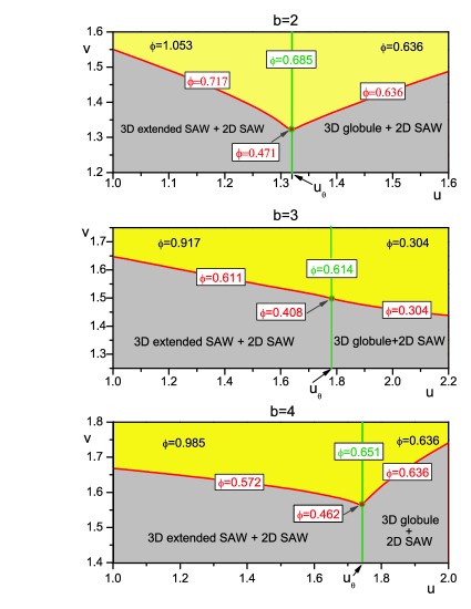
Figure 3: Phase diagrams obtained for the model of two avoiding SAWs on 3D SG fractals with $b=2,3$ and 4. The solid vertical line $u=u_{\theta}$ divides the $u-v$ plane in two areas, corresponding to the phases in which the 3D SAW is either extended ($u<u_{\theta}$) or collapsed ($u>u_{\theta}$). Each of these two areas is additionally partitioned by the critical line $v=v_{c}(u)$. For $v<v_{c}(u)$ the two polymers are segregated one from another, and the system exists either as “3D extended SAW + 2D SAW” for $u<u_{\theta}$, or “3D globule + 2D SAW” for $u>u_{\theta}$, whereas for $u=u_{\theta}$ precisely, $\theta$-chain coexists with 2D SAW. For $v\geq v_{c}(u)$ the mean number $\langle M\rangle$ of contacts between the two SAWs scales with the mean length $\langle N_{3}\rangle$ of the 3D SAW as $\langle M\rangle\sim\langle N_{3}\rangle^{\phi}$. Depending on the value of $u$, critical exponent $\phi$ has different values, which are presented within the corresponding areas.

Shape of the line $v_{c}(u)$, as well as values of the exponent $\phi$, show that the interplay between the intra- and inter-chain interactions in the system under study is quite subtle. In the $b=3$ case, $v_{c}(u)$ decreases monotonically with $u$, meaning that stronger monomer-monomer attraction within the $P_{3}$ chain eases its attaching to the $P_{2}$ chain. However, for $b=2$ and 4 fractals this is correct only for values of $u$ up to $u_{\theta}$, where $v_{c}(u)$ has its minimum. For larger values of $u$, function $v_{c}(u)$ monotonically increases with $u$, i.e. for $u>u_{\theta}$ intra-chain prevails inter-chain interaction and hinders attaching. Different behavior of the system on fractals with $b=2,4$ and $b=3$ is due to the peculiar topology of these lattices. Namely, although for $u>u_{\theta}$ polymer is in globular phase, compactness of that structure is not always the same. Only on $b=2$ SG the globule is completely compact, i.e. its fractal dimension $d_{f}^{G}$ is equal to the fractal dimension $d_{f}^{3D}$ of the lattice [21]. In the $b=3$ and 4 cases $d_{f}^{G}<d_{f}^{3D}$, but this quasi-compactness is much more pronounced in the $b=3$ case [22, 23], which brings about different behavior of the system on the $b=3$ SG fractal. Concerning the exponent $\phi$, which can be taken as a measure of interconnection between the two chains, one can notice that it has different values on the critical line $v_{c}(u)$ and in the region $v>v_{c}(u)$, and in addition depends on intra-chain interaction parameter $u$ (see table 1 and figure 3). For each of the three studied fractals, in the range $v>v_{c}(u)$ the inequality $\phi(u<u_{\theta})>\phi(u=u_{\theta})>\phi(u>u_{\theta})$ is satisfied. Such inequality could have been expected, since it means that when $P_{3}$ chain completely covers $P_{2}$ chain, the number of contacts between them is smaller if structure of the $P_{3}$ chain is more compact. On the line $v_{c}(u)$, however, chain $P_{2}$ is only partially covered with $P_{3}$, so that some similar conclusion is not plausible, which is indeed in accord with the calculated values of $\phi$. Besides, it is interesting that for $b=2$ and 4, the smallest value of $\phi$ is obtained for $u=u_{\theta}$, which is not the case for $b=3$ fractal.

Finally, one should note that in the case $b=3$, for the globular state of a solitary 3D chain ($u>u_{\theta}$), the coordinates of the corresponding fixed point are $A_{G}=0$ and $B_{G}=\infty$. Furthermore, a numerical analysis of function $D^{(r)}$, in the range $v\geq v_{c}(u)$ reveals that $D^{*}=\infty$. Nevertheless, the relation $\langle M^{(r)}\rangle\sim\lambda_{D}^{r}$ and formula (2.11) are applicable, but with different meaning of $\lambda_{D}$. For the globule state of $b=3$ fractal, it was demonstrated [22] that equations (1.5) and (1.6) in the vicinity of the corresponding fixed point $(0,\infty)$ have the following approximate form

$$A^{(r+1)}=320(A^{(r)})^{3}(B^{(r)})^{6}\,,\quad B^{(r+1)}=4308(A^{(r)})^{2}(B^{(r)})^{8}\>,$$ (2.12)

from which it follows $\lambda_{\nu_{3}}=\frac{\sqrt{73}+11}{2}=9.772$ and $\nu_{3}^{G}=\ln 3/\ln 9.772=0.4819$. Besides, for $v\geq v_{c}(u)$, the inequality $D^{(r)}\ll B^{(r)}$ is valid, so that RG equation (1.8) obtains the approximate form

$$D^{(r+1)}=320A^{(r)}(B^{(r)})^{6}C^{(r)}(D^{(r)})^{2}\,.$$ (2.13)

Then, from equations (2.7) and (2.8), follows $\langle M^{(r+1)}\rangle=2\frac{v}{D^{(r)}}\frac{\partial D^{(r)}}{\partial v}=2\langle M^{(r)}\rangle$, implying that $\langle M^{(r)}\rangle\sim\lambda_{D}^{r}$ (for large $r$), with $\lambda_{D}=2$. Finally, from (2.11), one obtains $\phi={\ln 2}/{\ln 9.772}=0.3041$.

3 The model of crossing walks

In order to describe the physical situation when closer contact between the two polymers is possible, in this section we analyze the CSAWs model in which chains $P_{2}$ and $P_{3}$ can cross each other [14]. If we assume that chains interact only at the crossing sites, and, similarly as in the ASAWs case, introduce the weight factor $w=e^{-\epsilon_{c}/k_{B}T}$, where $\epsilon_{c}\leq 0$ is the energy of two monomers in contact, it turns out that the two chains cannot exist independently, even for extremely weak attraction ($|\epsilon_{c}|\ll k_{B}T$). Therefore, we define additional weight factor $t=e^{-\epsilon_{t}/k_{B}T}$, where $\epsilon_{t}>0$ is the energy associated with two sites, visited by different SAWs, and both neighbouring a crossing site (see figure 1(b)), so that unbinding transition can occur. To describe exactly all possible configurations of the two-chain polymer system, within this model we need to introduce nine restricted partition functions: $A^{(r)}$, $B^{(r)}$, $C^{(r)}$, $A_{1}^{(r)}$, $A_{2}^{(r)}$, $A_{3}^{(r)}$, $A_{4}^{(r)}$, $B_{1}^{(r)}$, and $B_{2}^{(r)}$.

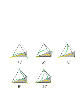
Figure 4: The six restricted generating functions used in the description of all possible inter-chain configurations for the CSAWs model of the two-polymer system, within the $r$-th stage of 3D SG fractal structure. The 3D chain is depicted by green line, while the 2D surface-adhered chain is depicted by yellow line.

Functions $A^{(r)}$, $B^{(r)}$ and $C^{(r)}$, which correspond to one-polymer configurations are the same as in the ASAWs model (see figure 2, and RG relations (2.2) and (2.3)), whereas the remaining six functions, which describe the inter-chain configurations, are depicted in figure 4, and they are defined as

$$A_{i}^{(r)} = \sum_{N_{2},N_{3},L,M,K}{\mathcal{A}}_{i}^{(r)}(N_{2},N_{3},L,M,K)x_{2}^{N_{2}}x_{3}^{N_{3}}u^{L}w^{M}t^{K}\,,\quad i=1,2,3,4\,,$$

$$B_{i}^{(r)} = \sum_{N_{2},N_{3},L,M,K}{\mathcal{B}}_{i}^{(r)}(N_{2},N_{3},L,M,K)x_{2}^{N_{2}}x_{3}^{N_{3}}u^{L}w^{M}t^{K}\,,\quad i=1,2\,,$$

where ${\mathcal{A}}_{i}^{(r)}$ and ${\mathcal{B}}_{i}^{(r)}$ are the numbers of particular two-polymer configurations on the $r$-th fractal structure. For instance, ${\mathcal{A}}_{4}^{(r)}(N_{2},N_{3},L,M,K)$ is the number of configurations in which the $N_{3}$-step $P_{3}$ chain (with $L$ intra-chain contacts) and $N_{2}$-step $P_{2}$ chain (with different entering end exiting vertices from $P_{3}$ chain) cross $M$ times and have $K$ pairs of sites belonging to different chains and neighboring the crossing sites. Functions $A_{i}^{(r)}$ and $B_{i}^{(r)}$ satisfy the following recursion relations

$$A^{\prime}_{i} = \sum_{\cal{N}}a_{i}({\cal{N}})\,A^{N_{A}}B^{N_{B}}C^{N_{C}}\prod_{j=1}^{4}A_{j}^{N_{A_{j}}}\prod_{k=1}^{2}B_{k}^{N_{B_{k}}}\,,\quad i=1,2,3,4\>,$$ (3.1)

$$B^{\prime}_{i} = \sum_{\cal{N}}b_{i}({\cal{N}})\,A^{N_{A}}B^{N_{B}}C^{N_{C}}\prod_{j=1}^{4}A_{j}^{N_{A_{j}}}\prod_{k=1}^{2}B_{k}^{N_{B_{k}}}\,,\quad i=1,2\>,$$ (3.2)

where $\cal{N}$ denotes the set of numbers ${\cal{N}}=\{N_{A},N_{B},N_{C},N_{A_{1}},N_{A_{2}},N_{A_{3},}N_{A_{4}},N_{B_{1}},N_{B_{2}}\}$, and where we have used the prime symbol as a superscript for $(r+1)$-th restricted partition functions and no indices for the $r$-th order partition functions. The above set of relations (3.1)–(3.2), together with the previously introduced relations (2.2)–(2.4) for the functions $A$, $B$, and $C$, can be considered as the system of RG equations for the problem under study, with the initial conditions

$$A^{(0)}=x_{3}\,,\quad B^{(0)}=x_{3}^{2}u^{4}\,,\quad C^{(0)}=x_{2}\,,$$

$$A_{1}^{(0)}=x_{3}x_{2}w^{2}\,,\quad A_{2}^{(0)}=A_{3}^{(0)}=x_{3}x_{2}wt\,,\quad A_{4}^{(0)}=x_{3}x_{2}\,,$$ (3.3)

$$B_{1}^{(0)}=B_{2}^{(0)}=x_{3}^{2}x_{2}w^{2}u^{4}\,,$$

corresponding to the unit tetrahedron. Because the number of all possible configurations is extremely large, we have been able to find explicit form of the RG equations (3.1)–(3.2) only for $b=2$ and $b=3$ SG fractals (see B). For both cases numerical analysis shows that, for each considered value of $t$, there is a critical line $w_{c}(u,t)$ dividing the $u-w$ plane into regions where the two polymers are either segregated ($w<w_{c}(u,t)$) or entangled ($w\geq w_{c}(u,t)$). Depending on the value of the intra-chain interaction parameter $u$, the area $w\leq w_{c}(u,t)$ is further partitioned into smaller regions, corresponding to various phases of the system (see figure  5).

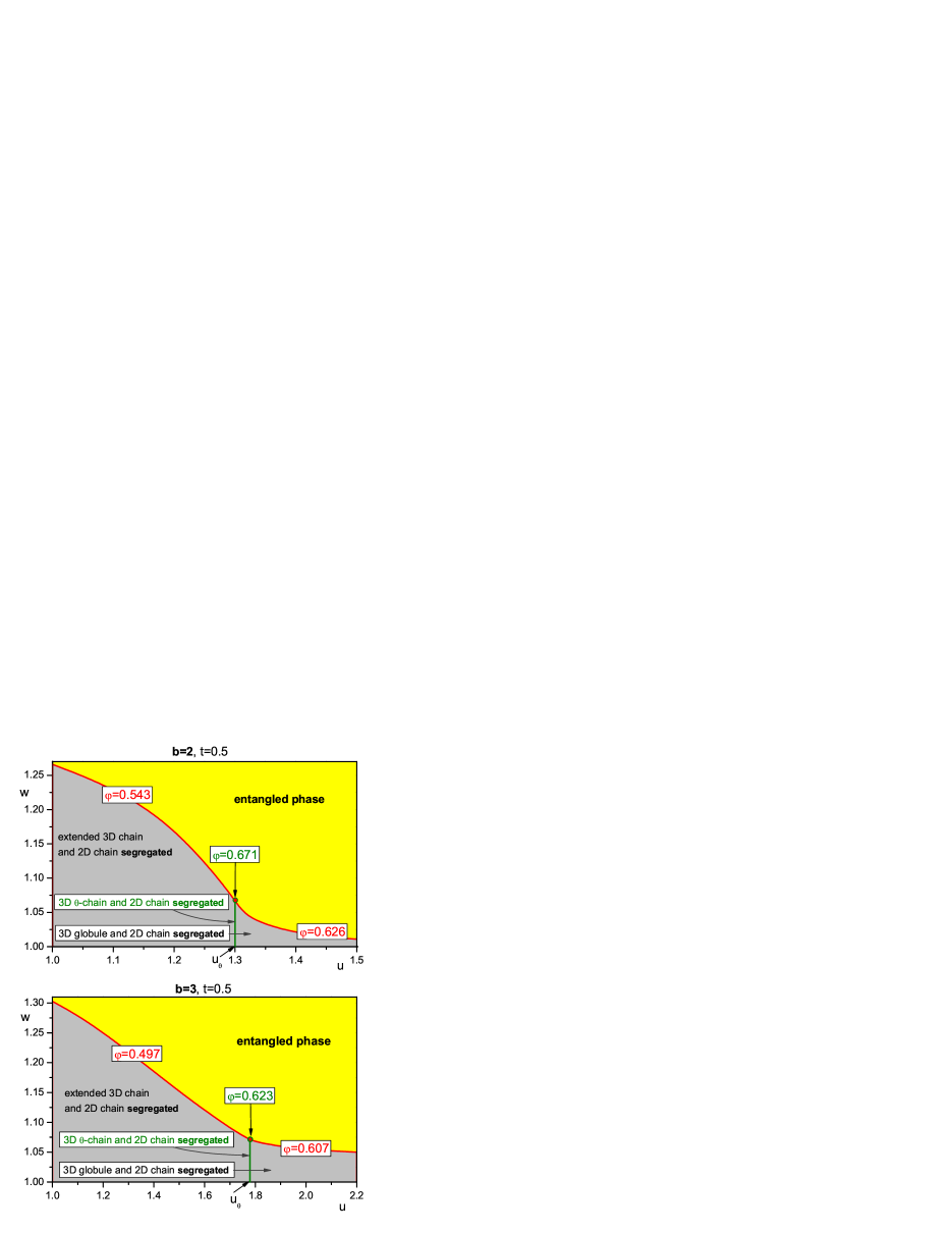
Figure 5: Phase diagrams in the space of interaction parameters for CSAWs model in the case of $b=2$ and $b=3$ SG fractal, for $t=0.5$. In both cases the critical line $w=w_{c}(u,t)$ separates the $u-w$ plane into the area $w>w_{c}(u,t)$ of entangled phase and area $w<w_{c}(u,t)$, in which the two chains are segregated. The latter area is divided by vertical line $u=u_{\theta}$ into regions, corresponding to three segregated phases: (i) 2D chain (always extended) and extended 3D chain ($u<u_{\theta}$), (ii) 2D chain and 3D $\theta$-chain ($u=u_{\theta}$), and (iii) 2D chain and 3D globule ($u>u_{\theta}$). One should observe that there appears the multi-critical point (full red circle) at the crossing of the $\theta$–line and the critical line $w=w_{c}(u,t)$. For other values of $t$ ($0<t<1$), the critical line $w_{c}(u,t)$ also monotonically decreases, for both $b=2$ and $b=3$ fractals.

To each of these area different fixed point of the general type

$$(A^{*},B^{*},C^{*},A_{1}^{*},A_{2}^{*},A_{3}^{*},A_{4}^{*},B_{1}^{*},B_{2}^{*})\>,$$ (3.4)

pertains. We describe general features of the fixed points and the corresponding phases in the three following subsections.

3.1 Weak self-attraction of the 3D chain

For each value of $0<t<1$, and small values of the interaction parameter $1\leq u<u_{\theta}$, there is some critical value $w=w_{c}(u,t)$ such that

• For $w<w_{c}(u,t)$ the fixed point of the form

  $$(A_{E},B_{E},C^{*},0,0,0,A_{4}^{*},0,0)\>,$$ (3.5)

  is reached. This point corresponds to the phase in which 2D chain and extended 3D chain are segregated, since as it is approached, after some number $r\gg 1$ of RG iterations, the average number of contacts between the two chains, quickly becomes constant. Values of $A_{E}$ and $B_{E}$ are fixed values of the RG parameters for the solitary extended chain on 3D SG fractal, and they are presented in table 2, together with the values of $C^{*}$, corresponding to 2D chain, which can exist only in extended state. RG fixed point value $A_{4}^{*}$ is equal to $0.1165$ and $0.0779$, for $b=2$ and 3 respectively, and they coincide with the values of $D^{*}$ for $v<v_{c}(u<u_{\theta})$ case in the ASAWs model (see table 1).

• For $w=w_{c}(u,t)$ one obtains the symmetrical fixed point

  $$(A_{E},B_{E},C^{*},A_{E}C^{*},A_{E}C^{*},A_{E}C^{*},A_{E}C^{*},B_{E}C^{*},B_{E}C^{*})\>,$$ (3.6)

  which appears to be a tricritical fixed point. As one approaches this fixed point, the average number of contacts ${\langle M^{(r)}\rangle}$ becomes infinitely large (although large parts of $P_{2}$ and $P_{3}$ are not in contact), and it turns out that it scales with the average length ${\langle{N_{3}}^{(r)}\rangle}$ of the 3D chain, according to the power law

  $${\langle M^{(r)}\rangle}\sim\langle{N_{3}}^{(r)}\rangle^{\varphi}\>.$$ (3.7)

  To calculate the contact critical exponent $\varphi$, within the CSAWs model, we find the average number of contacts between two chains at the $r$th stage of fractal construction, through the formula

  $$\langle M^{(r)}\rangle = {\sum_{N_{2},N_{3},L,M,K}M\left(\sum_{i=1}^{4}{\mathcal{A}}_{i}^{(r)}+{\sum_{j=1}^{2}{\mathcal{B}}_{i}^{(r)}}\right)x_{2}^{N_{2}}x_{3}^{N_{3}}u^{L}w^{M}t^{K}\over\sum_{i=1}^{4}A_{i}^{(r)}+\sum_{j=1}^{2}B_{j}^{(r)}}$$ (3.8)

  $$= {w\over\sum_{i=1}^{4}A_{i}^{(r)}+\sum_{j=1}^{2}B_{j}^{(r)}}\left(\sum_{i=1}^{4}\frac{\partial A_{i}^{(r)}}{\partial w}+\sum_{j=1}^{2}\frac{\partial B_{j}^{(r)}}{\partial w}\right)$$

  $$= {w\over\sum_{i=1}^{6}X_{i}^{(r)}}\sum_{i=1}^{6}\frac{\partial X_{i}^{(r)}}{\partial w}\>,$$

  where $X_{i}=A_{i}$ ($i=1,2,3,4$), $X_{5}=B_{1}$, and $X_{6}=B_{2}$. Since

  $$\frac{\partial X_{i}^{(r+1)}}{\partial w}=\sum_{j=1}^{6}\frac{\partial X_{i}^{(r+1)}}{\partial X_{j}^{(r)}}\frac{\partial X_{j}^{(r)}}{\partial w}\>,\quad i=1,\ldots,6\>,$$ (3.9)

  one expects, for large $r$, that $\frac{\partial X_{i}^{(r)}}{\partial w}$ behaves as $\lambda_{\varphi}^{r}$, where $\lambda_{\varphi}$ is the largest relevant solution of the eigenvalue equation

  $$\mbox{det}\left|\left({\partial X^{(r+1)}_{i}\over\partial X^{(r)}_{j}}\right)^{*}-\lambda_{\varphi}\,\delta_{ij}\right|=0\>,$$ (3.10)

  where the asterisk means that the derivatives should be taken at the tricritical fixed point. From here follows $\langle M^{(r)}\rangle\sim\lambda_{\varphi}^{r}$, which together with $\langle N_{3}^{(r)}\rangle\sim\lambda_{\nu_{3}}^{r}$ (where $\lambda_{\nu_{3}}$, as before, is the largest eigenvalue of the linearized RG equations for the bulk parameters $A$ and $B$), and (3.7), gives

  $$\varphi=\frac{\ln\lambda_{\varphi}}{\ln\lambda_{\nu_{3}}}\>.$$ (3.11)

• For larger values of the interaction parameter $w>w_{c}(u,t)$, the RG parameters flow towards the fixed point

  $$(0,0,0,A_{1}^{*}=C^{*},0,0,0,0,0)\>,$$ (3.12)

  which describes the entangled phase of the two polymers, in which $P_{3}$ chain is completely attracted to $P_{2}$ chain.

Table 2: The CSAWs model fixed points corresponding to the critical values $w=w_{c}(u,t)$ of the attraction parameter between the 2D and 3D chains, when $0<t<1$, for all possible states of the 3D polymer, together with the values of the critical exponent $\varphi$.

$b$	$A^{*}$	$B^{*}$	$C^{*}$	$A_{1}^{*}$	$A_{2}^{*}$	$A_{3}^{*}$	$A_{4}^{*}$	$B_{1}^{*}$	$B_{2}^{*}$	$\varphi$
extended 3D chain $(u<u_{\theta})$
2	0.4294	0.0499	0.6180	0.2654	0.2654	0.2654	0.2654	0.0308	0.0308	0.5428
3	0.3420	0.0239	0.5511	0.1884	0.1884	0.1884	0.1884	0.0131	0.0131	0.4973
3D $\theta$–chain $(u=u_{\theta})$
2	1/3	1/3	0.6180	0.0510	0	0	0.0613	0.2365	0.2362	0.6714
3	0.2071	0.4307	0.5511	0.0810	0.0310	0.0250	0.0270	0.3130	0.3150	0.6226
3D globule $(u>u_{\theta})$
2	0	0.3569	0.6180	0	0	0	0	0.2206	0.2206	0.6261
3	0	$\infty$	0.5511	0	0	0	0	$\infty$	$\infty$	0.6073

3.2 Critical self-attraction of the 3D chain

For $u=u_{\theta}$ the solitary 3D chain is in the state of the $\theta$-chain, for which $(A^{*},B^{*})=(A_{\theta},B_{\theta})$, whereas the two-polymer system can be in the following phases:

• For $w<w_{c}(u_{\theta},t)$ the corresponding fixed point is of the form

  $$(A_{\theta},B_{\theta},C^{*},0,0,0,A_{4}^{*},0,0)\>.$$ (3.13)

  This is the case when the 3D $\theta$-chain is segregated from the 2D chain chain. Fixed point values of $A_{4}^{*}$ are: 0.0613 for $b=2$, and 0.0211 for $b=3$ fractal, equal to $D^{*}$ for the corresponding cases $v<v_{c}(u_{\theta})$ of the ASAWs model.

• When $w=w_{c}(u_{\theta},t)$, the RG parameters tend to the fixed point

  $$(A_{\theta},B_{\theta},C^{*},A_{1}^{*},A_{2}^{*},A_{3}^{*},A_{4}^{*},B_{1}^{*},B_{2}^{*})\>,$$ (3.14)

  which corresponds to the phase in which chains are not segregated anymore, but they are not yet completely entangled. In contrast to the $w=w_{c}(u<u_{\theta},t)$ case, for which symmetrical fixed point is obtained, values of $A_{i}$ $(i=1,2,3,4)$, as well as $B_{1}$ and $B_{2}$, are not mutually equal ($A_{i}\neq A_{\theta}C^{*}$, $B_{i}\neq B_{\theta}C^{*}$). The scaling relation $\langle M^{(r)}\rangle\sim\langle{N_{3}}^{(r)}\rangle^{\varphi}$ is satisfied, with $\varphi$ given by (3.11).

• For $w>w_{c}(u_{\theta},t)$ the RG parameters flow towards the entangled fixed point (3.12).

3.3 Strong self-attraction of the 3D chain

When self-attraction of the 3D polymer is strong ($u>u_{\theta}$), depending on the values of inter-chain interaction parameters, the following phases are possible:

• For $w<w_{c}(u,t)$ the chains are segregated. Due to the large compactness of the 3D chain, with $(A^{*},B^{*})=(0,B_{G})$, none of the configurations $A_{1},A_{2},A_{3},A_{4},B_{1},B_{2}$ can be accomplished, and the corresponding fixed point is

  $$(0,B_{G},C^{*},0,0,0,0,0,0)\,.$$ (3.15)

  The chains are completely separated.

• When attraction between the chains is critical, $w=w_{c}(u,t)$, the chains are partially entangled, and the fixed point

  $$(0,B_{G},C^{*},0,0,0,0,B_{G}C^{*},B_{G}C^{*})\>,$$ (3.16)

  is attained. In this case the interaction between chains is sufficiently strong to connect them, but not strong enough to destroy the compactness of the 3D globule, so that all $A_{i}^{*}=0$. Again, the scaling relation $\langle M^{(r)}\rangle\sim\langle{N_{3}}^{(r)}\rangle^{\varphi}$ is satisfied for both $b=2$ and 3, with $\varphi$ given by (3.11). However, while in the case $b=2$ the coordinates of corresponding fixed point have definite values (and $\lambda_{\varphi}$ can be directly calculated from linearizied RG equations for $A_{i}$ and $B_{i}$), in the $b=3$ case some fixed point coordinates diverge, and calculation of $\lambda_{\varphi}$ requires an additional effort. To be more specific, a numerical analysis of RG equations (3.1) and (3.2) reveals that $A_{i}^{(r)}\approx A^{(r)}C^{*}\to 0$, $B_{i}^{(r)}\approx B^{(r)}C^{*}\to\infty$. In this situation the appropriate eigenvalue $\lambda_{\varphi}$ can also be calculated, using the following transformation. If we write the relation (3.9) in the form

  $${1\over X_{i}^{(r+1)}}\frac{\partial X_{i}^{(r+1)}}{\partial w}=\sum_{j=1}^{6}\left({X_{j}^{(r)}\over X_{i}^{(r+1)}}\frac{\partial X_{i}^{(r+1)}}{\partial X_{j}^{(r)}}\right){1\over X_{j}^{(r)}}\frac{\partial X_{j}^{(r)}}{\partial w}\>,\quad i=1,\ldots,6\>,$$ (3.17)

  it can be shown that, when we keep only dominant terms in the RG equations, and in the derivatives $\frac{\partial X_{i}^{(r+1)}}{\partial X_{j}^{(r)}}$, then, the matrix elements ${\left(\frac{X_{j}^{(r)}}{X_{i}^{(r+1)}}\frac{\partial X_{i}^{(r+1)}}{\partial X_{j}^{(r)}}\right)}^{*}$ of the new eigenvalue problem are either equal to zero or to some finite constants (depending on $C^{*}$), from which we find $\lambda_{\varphi}=3.9919$, and therefrom $\varphi={\ln\lambda_{\varphi}}/{\ln\lambda_{\nu_{3}}}=0.6073$.

• Strong inter-chain attraction $w>w_{c}(u,t)$ destroys the globule and completely attaches the 3D chain to the 2D chain. This entangled phase is again characterized by the fixed point (3.12).

In table 2 we have presented the numerical results for the crossover fixed points and the corresponding values of the contact exponent $\varphi$, obtained for the unbinding transitions from entangled two-polymer phase to segregated phases of 2D and 3D chains on the $b=2$ and $b=3$ 3D SG fractals. These values are correct for all studied cases of $t$ in the interval $(0,1)$. Varying the parameter $t$ in this interval changes only the particular values of $w_{c}(u,t)$, but, for both $b=2$ and $b=3$, the function $w_{c}(u,t)$ for fixed $t$ is monotonically decreasing function (see figure 5). Dependence of $w_{c}(u,t)$ on $t$, when $u$ is fixed, is presented in figure 6, for several values of $u$.

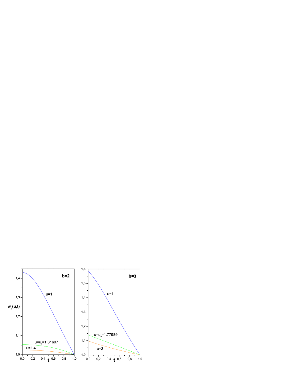
Figure 6: Critical value of the inter-chain interaction parameter $w_{c}(u,t)$, depicted as a function of $t$, for three different values of intra-chain interaction parameter $u$, in the cases of $b=2$ and $b=3$ 3D SG fractals.

As one can see, the limiting values $t=0$ and $t=1$ are also included in this figure. However, in these cases different fixed points, from those obtained for $0<t<1$, can be reached, which is expounded in the following paragraphs.

First, we analyze the value $t=0$, which represents the limiting case, within the CSAWs model, when the energy $\varepsilon_{t}$ (corresponding to the repelling of two different chain monomers, placed at sites which are nearest neighbours to a crossing site) is infinitely large. Starting with the initial values (3.3), it can be shown that, in the case of the $b=3$ fractal, the same fixed points of the RG equations (3.1) and (3.2), as for $0<t<1$ are reached. However, for the $b=2$ fractal, it can be seen, from the explicit form of the RG equations (2.1)–(2.6), that $t=0$ leads to $A_{2}^{(r)}=A_{3}^{(r)}=0$, for every $r$, $x_{2}$, $x_{3}$, $u$ and $w$. This is due to the topology of this fractal, and a consequence is that the fixed point $(A_{E},B_{E},C^{*},C^{*},0,0,A_{4}^{*},A_{4}^{*},0)$ corresponds to the critical values $w=w_{c}(1\leq u<u_{\theta},t=0)$. The coordinates of this fixed point $A_{E}=A^{*}$, $B_{E}=B^{*}$ and $C^{*}$ are given in the part “extended 3D chain ($u<u_{\theta}$)” of the table 2, while $A_{4}^{*}=0.1164$, and the concomitant critical exponent is $\varphi=0.8439$. The remaining fixed points are the same as for $0<t<1$.

The second limiting value ($t=1$) corresponds to the case $\varepsilon_{t}=0$ (when there is no repelling interaction). In this case, for all $u$, the critical value of the interaction parameter $w$ is equal to $w_{c}(u,t=1)=1$. This means that the chains can not be segregated, even for extremely small attraction between them. For both fractals $b=2$ and $b=3$, the fixed points that pertain to the critical value $w_{c}$, for $u\neq u_{\theta}$, are the same as for $0<t<1$. For $u=u_{\theta}$ the symmetrical fixed point is reached, $(A_{\theta},B_{\theta},C^{*},A_{\theta}C^{*},A_{\theta}C^{*},A_{\theta}C^{*},A_{\theta}C^{*},B_{\theta}C^{*},B_{\theta}C^{*})$, in contrast to the case $0<t<1$. Values of $A_{\theta}=A^{*}$, $B_{\theta}=B^{*}$ and $C^{*}$ can be found in the middle part of the table 2, while the values of the contact critical exponents are $\varphi(b=2)=0.6102$, and $\varphi(b=3)=0.5907$.

Finally, one should mention that recently, using the Monte Carlo renormalization group (MCRG) method, the contact exponent $\varphi$ was calculated for $b$ up to 40, for the case when the intra-chain interactions within the 3D chain are negligible, $u\to 0$ [14]. Comparing the reported MCRG data $\varphi^{MC}(b=2)=0.5440\pm 0.0056$ and $\varphi^{MC}(b=3)=0.4969\pm 0.0024$ with our exact findings $\varphi(b=2)=0.5428$ and $\varphi(b=3)=0.4973$, we can see that MCRG data are in excellent agreement with our exact findings. In [14] it was also demonstrated that $\varphi^{MC}$, as a function of the scaling parameter $b$, continues decreasing with increasing $b$, and, it seems that in the fractal-to-Euclidean crossover region (i.e. in the limit $b\to\infty$) it goes to the proposed zero Euclidean value. The inequality $\varphi(b=2)>\varphi(b=3)$ is satisfied not only for weak intra-chain interactions ($u<u_{\theta}$), but also for $u\geq u_{\theta}$, as can be seen in table 2. Unfortunately, in the range $u\geq u_{\theta}$, the MCRG calculation of $\varphi$ is not feasible, so that prediction for the large $b$ behavior of $\varphi(u\geq u_{\theta})$, only on the bases of our exact data, is not possible.

4 Summary and conclusion

In this paper we have studied a system of two interacting chemically different polymer chains in a poor solvent. Such a situation can be modelled by two avoiding self-avoiding walks (ASAWs), as well as by two crossing self-avoiding walks (CSAWs). We assume that polymers are situated in fractal containers modelled by members of 3D SG fractal family, which are labelled by an integer $b$ ($2\leq b<\infty$). We adopt that the first polymer ($P_{3}$) is a floating chain in the bulk of 3D SG fractal, while the second ($P_{2}$) is stuck to one of the four boundaries of the 3D SG fractal, which appears to be a 2D SG fractal. To take into account the intra-chain interaction of $P_{3}$ polymer we have introduced the interaction parameter $u={\mathrm{e}}^{-\varepsilon_{u}/k_{B}T}$, where $\varepsilon_{u}<0$ is the energy corresponding to interaction between two nonconsecutive neighboring monomers within the chain. In the case of ASAWs model, the two SAW paths cannot intersect each other, and we assume that two polymers interact when they approach a distance equal to a lattice constant. We associate the weight factor $v=e^{-\epsilon_{v}/k_{B}T}$ with each such contact, where $\epsilon_{v}<0$ is the appropriate energy of inter-chain interaction. On the other hand, in the case of CSAWs model, in order to describe the inter-chain interactions of $P_{3}$ and $P_{2}$, we have introduced the parameters $w={\mathrm{e}}^{-\varepsilon_{c}/k_{B}T}$ and $t={\mathrm{e}}^{-\varepsilon_{t}/k_{B}T}$, where $\epsilon_{c}<0$ is the energy corresponding to each crossing of SAWs, while $\epsilon_{t}>0$ is the energy associated with a pair of sites, visited by different SAWs, which are nearest neighbors to a crossing site.

To obtain the phase diagrams and the contact critical exponents between the two polymers, we have applied an exact RG method for the 3D SG fractals labelled by $b=2,3$ and 4, in the case of ASAWs model, and for fractals $b=2$ and 3, in the case of CSAWs model. In both models, for various values of intra-chain interaction parameter $u$, a solitary 3D floating polymer chain can be found in one of the three possible phases (extended, $\theta$-phase, or globule phase), whereas a solitary 2D chain is always extended. Depending on the values of the inter-chain interaction parameters ($v$ in the case of ASAWs model, and $w$ and $t$ in the case of CSAWs model), the system can be either in the segregated phase, when the chains can be considered as almost independent, or in phases in which the number of contacts between the chains is comparable with their length (entangled phases). For both models, there is a critical line in the plane of the interaction parameters ($v_{c}(u)$ for ASAWs, and, $w_{c}(u,t)$, with fixed $t$, for CSAWs model), which divides it into areas corresponding to segregated and entangled phases. In the case of the ASAWs model, for $v\geq v_{c}(u)$, the average number $\langle M\rangle$ of contacts between the two polymers scales with the average length $\langle N_{3}\rangle$ of the 3D chain as $\langle M\rangle\sim{\langle N_{3}\rangle}^{\phi}$. Different values of the contact exponent $\phi$ correspond to $v=v_{c}(u)$ and $v>v_{c}(u)$, and, in addition, $\phi$ also depends on the strength of the intra-chain interaction parameter $u$. However, in all entangled phases large parts of the 3D chain remain in the bulk, beyond the scope of the inter-chain interaction, since the prohibition of crossings between two chains hinders their complete entanglement, even for extremely large values of $v$. On the contrary, in CSAWs model for $w>w_{c}(u,t)$ the two chains are completely entangled, while they only partially cover each other at the critical line $w=w_{c}(u,t)$, where the scaling relation $\langle M\rangle\sim{\langle N_{3}\rangle}^{\varphi}$ is satisfied, and where $\varphi$ takes different values in the intra-chain interaction regions $u<u_{\theta}$, $u=u_{\theta}$, and $u>u_{\theta}$.

In the end, we would like to point out that for ASAWs model, in the space of interaction parameters, the arrangement of possible phases is approximately the same, as in the case of the surface-interacting polymer chain in a poor solvent in Euclidean spaces [15, 16, 17]. On the other hand, the obtained phase diagrams for CSAWs model, resemble the phase diagrams of the same surface-interacting chain problem, in fractal containers [23]. This similarity is not surprising, since in both models studied, one of the two interacting polymers is adhered to one of four fractal surfaces, and its monomers appear as a part of interacting surface (in the surface-interacting polymer problem). Here we may conclude that, our findings should be useful in making the corresponding 3D models of the system of several interacting polymer chains in porous media. Besides, our results may serve inspiring in advancing theories of mutually interacting polymers, as well as for polymers interacting with boundary surfaces of homogeneous 3D lattices, in which case so far (to the best of our knowledge) an exact approach has not been yet made.

Appendix A Renormalization group equations for the ASAWs model

In this Appendix we give explicit RG equations for the model in which two chains avoid each other, for the cases $b=2$, and $b=3$ of 3D SG fractals. Equations for “bulk” parameters $A$ and $B$, as well as for the “surface” parameter $C$, were found in earlier works, and we give them here only for the sake of completeness.

First, we give the RG equations for $b=2$ 3D SG fractal

$$A^{\prime} = A^{2}+2\,A^{3}+2\,A^{4}+4\,A^{3}\,B+6\,A^{2}\,B^{2}\,,$$ (1.1)

$$B^{\prime} = A^{4}+4\,A^{3}\,B+22\,B^{4}\,,$$ (1.2)

$$C^{\prime} = C^{2}+C^{3}\,,$$ (1.3)

$$D^{\prime} = 2\,{D}^{3}\,B+6\,{D}^{2}\,B^{2}+2\,A^{2}\,D\,C+A^{2}\,C^{2}+A\,D\,C^{2}\,.$$ (1.4)

We note that first three equations were established for the first time in [19].

Next, we present RG equations for the $b=3$ case

$$A^{\prime} = A^{3}+6A^{4}+16A^{5}+34A^{6}+76A^{7}+112A^{8}+112A^{9}+64A^{10}+8A^{4}B+36A^{5}B$$ (1.5)

$$+ 140A^{6}B+292A^{7}B+424A^{8}B+332A^{9}B+12A^{3}B^{2}+12A^{4}B^{2}+118A^{5}B^{2}$$

$$+ 380A^{6}B^{2}+806A^{7}B^{2}+664A^{8}B^{2}+72A^{4}B^{3}+352A^{5}B^{3}+704A^{6}B^{3}+1728A^{7}B^{3}$$

$$+ 344A^{4}B^{4}+1568A^{5}B^{4}+848A^{6}B^{4}+264A^{4}B^{5}+3192A^{5}B^{5}+320A^{3}B^{6}\,,$$

$$B^{\prime} = A^{6}+12A^{7}+40A^{8}+60A^{9}+32A^{10}+28A^{6}B+88A^{7}B+224A^{8}B+160A^{9}B$$ (1.6)

$$+ 40A^{6}B^{2}+496A^{7}B^{2}+596A^{8}B^{2}+176A^{5}B^{3}+768A^{6}B^{3}+1056A^{7}B^{3}+88A^{3}B^{4}$$

$$+ 264A^{5}B^{4}+2534A^{6}B^{4}+1152A^{4}B^{5}+1888A^{5}B^{5}$$

$$+ 5808A^{4}B^{6}+1936A^{3}B^{7}+4308A^{2}B^{8}\,,$$

$$C^{\prime} = C^{3}+3C^{4}+C^{5}+2C^{6}\,,$$ (1.7)

$$D^{\prime} = 2A^{6}D^{3}+4A^{7}D^{3}+4A^{6}D^{4}+2A^{5}D^{5}+28A^{6}D^{3}B+4A^{4}D^{4}B+14A^{5}D^{4}B$$ (1.8)

$$+ 4A^{4}D^{5}B+8A^{4}D^{3}B^{2}+56A^{5}D^{3}B^{2}+44A^{4}D^{4}B^{2}+4A^{3}D^{5}B^{2}$$

$$+ 144A^{4}D^{3}B^{3}+36A^{3}D^{4}B^{3}+12A^{2}D^{5}B^{3}+72A^{3}D^{3}B^{4}+132A^{2}D^{4}B^{4}$$

$$+ 264A^{2}D^{3}B^{5}+12A^{6}D^{2}C+18A^{7}D^{2}C+2A^{4}D^{3}C+8A^{5}D^{3}C+8A^{6}D^{3}C$$

$$+ 4A^{5}D^{4}C+2A^{4}D^{5}C+16A^{4}D^{2}BC+48A^{5}D^{2}BC+64A^{6}D^{2}BC$$

$$+ 4A^{2}D^{3}BC+8A^{4}D^{3}BC+48A^{5}D^{3}BC+4A^{3}D^{4}BC+8A^{4}D^{4}BC$$

$$+ 8A^{3}D^{5}BC+12A^{2}D^{2}B^{2}C+36A^{4}D^{2}B^{2}C+162A^{5}D^{2}B^{2}C+24A^{3}D^{3}B^{2}C$$

$$+ 28A^{4}D^{3}B^{2}C+44A^{3}D^{4}B^{2}C+8A^{2}D^{5}B^{2}C+96A^{3}D^{2}B^{3}C+64A^{4}D^{2}B^{3}C$$

$$+ 152A^{3}D^{3}B^{3}C+24A^{2}D^{4}B^{3}C+24AD^{5}B^{3}C+512A^{3}D^{2}B^{4}C$$

$$+ 88AD^{4}B^{4}C+264A^{2}D^{2}B^{5}C+320AD^{2}B^{6}C+6A^{4}DC^{2}+16A^{5}DC^{2}$$

$$+ 28A^{6}DC^{2}+12A^{7}DC^{2}+12A^{5}D^{2}C^{2}+18A^{6}D^{2}C^{2}+2A^{3}D^{3}C^{2}$$

$$+ 6A^{4}D^{3}C^{2}+8A^{5}D^{3}C^{2}+4A^{4}DBC^{2}+64A^{5}DBC^{2}+56A^{6}DBC^{2}$$

$$+ 12A^{3}D^{2}BC^{2}+30A^{4}D^{2}BC^{2}+36A^{5}D^{2}BC^{2}+2AD^{3}BC^{2}+6A^{3}D^{3}BC^{2}$$

$$+ 24A^{4}D^{3}BC^{2}+100A^{4}DB^{2}C^{2}+88A^{5}DB^{2}C^{2}+6AD^{2}B^{2}C^{2}$$

$$+ 18A^{3}D^{2}B^{2}C^{2}+56A^{4}D^{2}B^{2}C^{2}+4A^{2}D^{3}B^{2}C^{2}+20A^{3}D^{3}B^{2}C^{2}$$

$$+ 160A^{4}DB^{3}C^{2}+36A^{2}D^{2}B^{3}C^{2}+32A^{2}D^{3}B^{3}C^{2}+256A^{3}DB^{4}C^{2}$$

$$+ 132A^{2}D^{2}B^{4}C^{2}+44AD^{3}B^{4}C^{2}+A^{3}C^{3}+6A^{4}C^{3}+10A^{5}C^{3}+10A^{6}C^{3}$$

$$+ 6A^{7}C^{3}+8A^{3}DC^{3}+10A^{4}DC^{3}+14A^{5}DC^{3}+10A^{6}DC^{3}$$

$$+ 4A^{4}D^{2}C^{3}+6A^{5}D^{2}C^{3}+2A^{3}D^{3}C^{3}+6A^{4}D^{3}C^{3}+8A^{4}BC^{3}+16A^{5}BC^{3}$$

$$+ 20A^{6}BC^{3}+28A^{4}DBC^{3}+36A^{5}DBC^{3}+8A^{3}D^{2}BC^{3}+12A^{4}D^{2}BC^{3}$$

$$+ 4A^{2}D^{3}BC^{3}+16A^{3}D^{3}BC^{3}+12A^{3}B^{2}C^{3}+18A^{5}B^{2}C^{3}+12A^{2}DB^{2}C^{3}$$

$$+ 44A^{4}DB^{2}C^{3}+12A^{3}D^{2}B^{2}C^{3}+20A^{2}D^{3}B^{2}C^{3}+24A^{4}B^{3}C^{3}$$

$$+ 48A^{3}DB^{3}C^{3}+24A^{2}D^{2}B^{3}C^{3}+24AD^{3}B^{3}C^{3}+3A^{3}C^{4}+10A^{4}C^{4}$$

$$+ 10A^{5}C^{4}+4A^{6}C^{4}+A^{2}DC^{4}+2A^{3}DC^{4}+2A^{4}DC^{4}+12A^{4}BC^{4}$$

$$+ 8A^{5}BC^{4}+4A^{3}DBC^{4}+18A^{3}B^{2}C^{4}+6A^{2}DB^{2}C^{4}+2A^{2}DC^{5}$$

$$+ 4A^{3}DC^{5}+4A^{4}DC^{5}+8A^{3}DBC^{5}+12A^{2}DB^{2}C^{5}\>.$$

Equations (1.5) and (1.6) were found in [22], and (1.7) in [20].

For the $b=4$ case, equations are too cumbersome to be quoted here, and, they are available upon request to the authors.

Appendix B Renormalization group equations for the CSAWs model

It can be shown, via direct computer enumeration of the corresponding paths within the generator of the $b=2$ 3D SG fractal, that RG parameters $A_{1},A_{2},A_{3},A_{4},B_{1}$, and $B_{2}$ fulfil the following recursion relations

$$A^{\prime}_{1} = A_{1}^{2}+A_{1}^{3}+A{A_{2}^{2}}+2A^{2}A_{2}A_{3}+A{A_{3}^{2}}+2AA_{1}{A_{3}^{2}}+2AA_{2}A_{3}B_{1}+2AA_{2}A_{3}B_{2}$$ (2.1)

$$+ 4A^{2}A_{1}B_{2}+4A^{2}B_{1}B_{2}+4AA_{1}B_{1}B_{2}+2A^{2}{B_{2}^{2}}+2AA_{1}{B_{2}^{2}}+{A_{2}^{2}}C+A{A_{3}^{2}}C\>,$$

$$A^{\prime}_{2} = AA_{1}A_{2}+A_{2}^{3}+A^{2}A_{1}A_{3}+AA_{2}A_{3}^{2}+A^{2}A_{3}A_{4}+AA_{2}A_{4}^{2}+2AA_{2}A_{4}B+AA_{3}A_{4}C$$ (2.2)

$$+ A^{2}A_{3}B_{1}+AA_{1}A_{3}B_{1}+2AA_{2}BB_{1}+AA_{2}B_{1}^{2}+A^{2}A_{3}B_{2}+4AA_{2}BB_{2}+A^{2}A_{3}C$$

$$+ 2AA_{2}B_{1}B_{2}+3AA_{2}B_{2}^{2}+AA_{2}C+A_{1}A_{2}C+AA_{1}A_{3}B_{2}+2AA_{2}A_{4}B_{2}\,,$$

$$A^{\prime}_{3} = A^{2}A_{1}A_{2}+AA_{1}A_{3}+AA_{1}^{2}\,A_{3}+AA_{2}^{2}A_{3}+A^{2}A_{2}A_{4}+2A_{3}^{3}B+4AA_{3}BB_{2}+AA_{3}C^{2}$$ (2.3)

$$+ 2AA_{3}A_{4}B+A^{2}A_{2}B_{1}+AA_{1}A_{2}B_{1}+2AA_{3}BB_{1}+2A_{3}A_{4}BB_{1}+AA_{2}A_{4}C$$

$$+ A^{2}A_{2}B_{2}+4A_{3}A_{4}BB_{2}+A^{2}A_{2}C+AA_{3}C+AA_{1}A_{3}C+AA_{1}A_{2}B_{2}\,,$$

$$A^{\prime}_{4} = 2A^{2}A_{2}A_{3}+2AA_{2}^{2}A_{4}+2AA_{2}^{2}B+2AA_{3}^{2}\,B+2A_{4}^{3}B+6A_{4}^{2}B^{2}+2A_{3}^{2}BB_{1}$$ (2.4)

$$+ 2AA_{2}^{2}B_{2}+4A_{3}^{2}BB_{2}+2AA_{2}A_{3}C+2A^{2}A_{4}C+A^{2}C^{2}+AA_{4}C^{2}\,,$$

$$B^{\prime}_{1} = A^{2}A_{1}^{2}+AA_{2}^{2}A_{4}+AA_{2}^{2}B+AA_{3}^{2}B+A_{3}^{2}A_{4}B+2A^{2}A_{1}B_{1}+AA_{1}^{2}B_{1}+8BB_{2}^{3}$$ (2.5)

$$+ 6B^{2}B_{1}^{2}+2BB_{1}^{3}+2AA_{2}^{2}B_{2}+8B^{2}B_{1}B_{2}+4BB_{1}^{2}B_{2}+8B^{2}B_{2}^{2}+8BB_{1}B_{2}^{2}\,,$$

$$B^{\prime}_{2} = A^{2}A_{2}A_{3}+AA_{1}A_{2}A_{3}+AA_{2}^{2}B+AA_{3}^{2}B+A_{3}^{2}A_{4}B+AA_{2}^{2}B_{1}+10BB_{1}B_{2}^{2}+6BB_{2}^{3}$$ (2.6)

$$+ 2A^{2}A_{1}B_{2}+AA_{1}^{2}B_{2}+AA_{2}^{2}B_{2}+12B^{2}B_{1}B_{2}+6BB_{1}^{2}B_{2}+10B^{2}B_{2}^{2}\,.$$

One can check, by inserting $A_{1}=A_{2}=A_{3}=B_{1}=B_{2}=0$ and $A_{4}=D$, into equation (2.4) for the function $A_{4}$, that RG equation (1.4) for the function $D$ in the case of the ASAWs model is recovered. This is not surprising, since it follows from the definitions of $A_{4}$ and $D$, and it is certainly also correct for the $b=3$ fractal equations. However, here we do not quote the $b=3$ RG equations because they are extremely intricate. For instance, equation for the parameter $A_{1}$ has 2753 terms, and it is similar for the remaining $A_{i}$ and $B_{i}$ equations.

References

References

- [1] Vanderzande C, 1998 Lattice Models of Polymers, Cambridge: Cambrige University Press
- [2] Pelissetto A and Vicari E, 2006 Phys. Rev. E 73 051802
- [3] Orlandini E, Seno F and Stella A L, 2000 Phys. Rev. Lett. 84 294
- [4] Baiesi M, Carlon E, Orlandini E and Stella A L, 2001 Phys. Rev. E 63 041801
- [5] Marenduzzo D, Bhattacharjee S M, Maritan A, Orlandini E and Seno F, 2002 Phys. Rev. Lett. 88 028102
- [6] Kapri R and Bhattacharjee S M, 2006 J. Phys.: Condens. Matter 18 S215
- [7] Giri D and Kumar S, 2006 Phys. Rev. E 73 050903(R)
- [8] Kapri R and Bhattacharjee S M, 2007 Phys. Rev. Lett. 98 098101
- [9] Kumar S and Singh Y, 1993 J. Phys. A: Math. Gen. 26 L987
- [10] Kumar S and Singh Y, 2001 Physica A 293 345
- [11] Leoni P, Vanderzande C and Vandeurzen J, 2001 J. Phys. A: Math. Gen. 34 9777
- [12] Mukherji S and Bhattacharjee S M 1995 Phys. Rev. E 52 1930
- [13] Haddad T A S, Andrade R F S and Salinas S R, 2004 J. Phys. A: Math. Gen. 37 1499
- [14] Živić I, 2007 J. Stat. Mech. P02005
- [15] Singh Y, Giri D and Kumar S, 2001 J. Phys. A: Math. Gen. 34 L67
- [16] Rajesh R, Dhar D, Giri D, Kumar S and Singh Y, 2002 Phys. Rev. E 65 056124
- [17] Owczarek A L, Rechnitzer A, Krawczyk J and Prellberg T, 2007 J. Phys. A: Math. Gen. 40 13257
- [18] Usatenko Z and Sommer J-U, 2007 J. Stat. Mech. P10006
- [19] Dhar D, 1978 J. Math. Phys. 19 5
- [20] Elezović S, Knežević M and Milošević S, 1987 J. Phys. A: Math. Gen. 20 1215
- [21] Dhar D and Vannimenus J, 1987 J. Phys. A: Math. Gen. 20 199
- [22] Knežević M and Vannimenus V, 1987 J. Phys. A: Math. Gen. 20 L969
- [23] Elezović-Hadžić S, Živić I and Milošević S, 2003 J. Phys. A: Math. Gen. 36 1213