Applications of physical methods in high-frequency futures markets

Abstract

In the present work we demonstrate the application of different physical methods to high-frequency or tick-by-tick financial time series data. In particular, we calculate the Hurst exponent and inverse statistics for the price time series taken from a range of futures indices. Additionally, we show that in a limit order book the relaxation times of an imbalanced book state with more demand or supply can be described by stretched exponential laws analogous to those seen in many physical systems.

1 Introduction

In recent years the study of financial markets have become more prevalent among the physics community[1, 2, 3]. The popularity of this area of research, also known as econophysics, is partially due to the large amount of data that has become freely available to scientists. However, most of the studies deal with sample periods of the order of days while in fact a large number of modern financial institutions often deal with high-frequency or tick-by-tick data.

The importance of tick-by-tick time series data is certainly related to the fact that it allows one to address important questions regarding the dynamics of market microstructure. One such question relates to the possible presence of higher-order or non-linear correlations in the price change dynamics, quantities that can be characterised by calculation of the Hurst exponent [4], $H\in[0,1]$, of the time series. If non-linear correlations are identified then they can be seen as a possible source of price feedback or market inefficiency and as such serve to contradict the efficient market hypothesis (EMH) [5]. Such things are very interesting for market participants who might, for example, seek to construct high-frequency trading systems. Related to the presence of high-order correlations are questions about the nature of first passage distribution of the price time series. Investigations into the first passage time can be placed within the framework of inverse statistics [6, 7] and are another tool for understanding the scaling properties of a times series. Alternatively, for a high-frequency trader, knowledge of the first passage distribution is useful in that it can be used to construct estimates of the optimal investment horizon, $\tau$, that is, the average time required for the price to move by some specified amount. For Brownian motion, the analytical solution for $P(\tau)$, the distribution of $\tau$, is known [8, 9, 10]. For price evolution that is non-Brownian (possibly due to high-order correlations) an empirical model for $P(\tau)$ will need to be derived. Another set of interesting microstructure questions can be posed around understanding the dynamics of the limit order book. The limit order book stores market supply and demand and generally exists in a state of disequilibrium. In fact, there are complex interplays and feedbacks between the evolution of the order book state, the order flow in the market, and the evolution of the market price. Hence arriving at an understanding of the order book dynamics is important if we are to attempt a complete explanation of the observed price change dynamics.

In this work we investigate higher-order correlations within financial time series by calculating the local Hurst exponent, $H_{L}(t)$, for a range of futures markets. The interest in the local Hurst exponent is that it allows one to investigate how scaling within a time series varies in time and with length scale. For the same markets we investigate also the distribution of the first passage time and fit an empirical model to describe the distribution of the optimal investment horizon $P(\tau)$. Finally, we study some characteristics of the relaxation of volume imbalances in limit order books. Specifically, we look at the distribution of times that an unbalanced limit order book book takes to revert to a zero imbalance or equilibrium state.

2 Local behaviour of Hurst exponents in high-frequency futures contracts

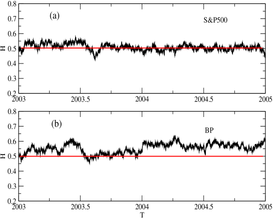
In physics, as well as other scientific disciplines, the Hurst exponent, $H\in[0,1]$, is often considered as an indicator for correlations in time series analysis [4]. In particular, for $0\leq H<0.5$ it is said that the behaviour of the time series is antipersistent, and conversely, persistent for $0.5<H\leq 1$. For completely uncorrelated movements, as assumed by the “efficient market hypothesis” of financial markets, we expect $H=0.5$. As a first step of our investigation we apply the concept of local Hurst exponent, $H_{L}(t)$, to different time series of futures contracts sampled at 1 minute period from 1/1/2003 and ending 31/12/2004. According to this method, described in Ref. [11], the exponent $H$ is calculated, via the detrended fluctuation analysis [12] (DFA), over a time window of length $L$ much smaller of the length of the entire time series. The calculation is then repeated by shifting the time window by a fixed period (in the present analysis 10 minutes) so to obtain an entire time series of Hurst exponents. An example of the outcome of this method is given in Fig. 1 where the time series of $H_{L}(t)$ for the S&P500 (SP) and the British Pound exchange rate (BP) futures indices are reported. From the plot, we can notice how the Hurst exponent is not strictly stationary during the period under consideration. However for the S&P500, Fig. 1 (top), the values of $H_{L}(t)$ are always very close to $0.5$ (apart from a few periods) and, considering the error over their values, there is no evidence for long periods of persistency or antipersistency at this temporal scale. The same does not hold for the BP, Fig. 1 (bottom), where significant deviations from the random walk behaviour can be observed. Further examples are reported in Ref. [11].

Figure 1: Time series of local Hurst exponents, $H_{L}(t)$, for the time series S&P500 (SP)(a) and British Pound exchange rate (BP) (b) on a scale of approximately 16 days ($L=8192$) and constant shift $\Delta t=10$ minutes. For the SP, a particularly liquid market $H$, is always very close to 0.5, irrespective of the particular period under consideration. The time period goes from 1/1/2003 to 31/12/2004. The BN, instead, displays periods in which H is significantly different from the random walk benchmark.

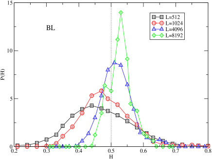
The general statistical behaviour of the local Hurst exponent is not only sensitive to the particular market but also to the scale of the observation. In order to highlight these differences we report in Fig. 2 the pdfs of $H_{L}(t)$ for various $L$ in the particular case of the BOBL. For this fixed contract it is evident a change in the average behaviour of the index: from persistent at large scales to anti-persistent at small scales.

Figure 2: The pdfs for the BOBL (BL) futures show a quite singular behaviour. The index seems to shift from a slightly persistent to a slightly antipersistent behaviour as we move toward smaller scales.

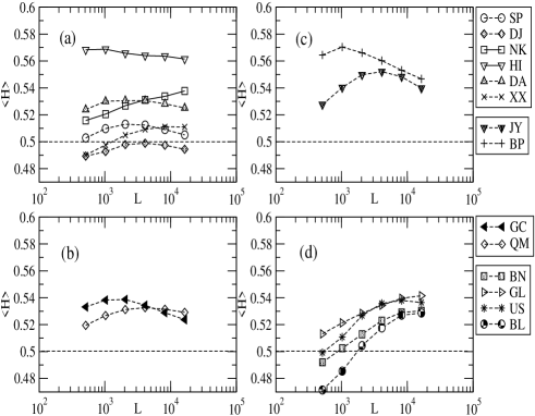
The relationship between the market dynamics and the scale of observation appears to become more evident when we plot the average value of the local Hurst exponent, $\langle H\rangle$, against the scale $L$, Fig. 3, ranging from 32 to 1 working days approximately. From this graph we infer how time series belonging to the same sector tend to have a qualitatively similar scale dependency. The indices futures, for example, Fig. 3 (a), do not display a strong correlation between $\langle H\rangle$ and $L$ with the exception of the Hang Seng (HI) whose persistency increases sharply at smaller scales. On the other hand a scale dependency is quite evident for the fixed income products, Fig. 3 (d), where, interestingly, some time series (BN, US and BL) move from an antipersistent-like to an persistent-like behaviour as the scale increases.

Figure 3: Average value of the local Hurst exponent, $\langle H\rangle_{L}$, for index futures, DAX (DA), Euro Stoxx (XX), Standard & Poor500 (SP), Dow (DJ), Hang Seng (HI) and Nikkei255 (a), commodity futures, Gold COMEX (GC) and Crude Oil E-mini (QM) (b), exchange rate futures, Japanese Yen (JY) and British Pound (BP) (c) and fixed income futures, Eurex Bunds (BN), Long Gilts (GL), Treasury Bonds (US) and BOBL (BL) (d). The horizontal dotted line is set at 0.5 for visual reference.

As a result of the analysis carried out in this section we can claim that the actual behaviour of the stock market, described in terms of Hurst exponent, apart from being influenced by the particular period of time under consideration and by the maturity of the market [13, 14, 15, 16, 17], is also related to the scale of observation: this is an extremely relevant issue for practical applications. In fact, if we consider long time scales (large $L$), in reality, we are estimating the average Hurst exponent over that period.

For more exhaustive discussion on this subject and on “pitfalls” of the method with high-frequency data we refer the reader to Ref. [11].

3 Optimal exit times in futures indices at tick level

The framework of inverse statistics has been recently introduced in the context of hydrodynamics with the aim of investigating the scaling properties of the elapsed times between large fluctuations in the velocity field of turbulent flows [6, 7]. Given the analogies between the scaling in turbulence and in the stock market dynamics [5, 18, 2, 3], the application of this technique has been consequently extended to finance [19, 20, 21, 22, 23].

The inverse statistics method consists in calculating, for each element of a time series, the time interval, or exit time, needed in order to reach for the first time a certain target level, $R$. For a generic variable $Y$ at time $t$, the exit time, $\tau_{R}(t)$, can be formally defined as

$$\tau_{R}(t)={\rm inf}\{T>0\,|\,Y(t+T)-Y(t)\geq R\}.$$ (1)

For clarity of notation, in the rest of the paper we will indicate the exit time simply as $\tau$.

The first passage distribution, $P(\tau)$, is then the probability distribution function (pdf) of the exit times. In the financial context we can identify the variable $Y(t)$ with the price of a certain index, $p_{r}(t)$, or, alternatively, with its logarithm. In previous studies [19, 20, 21, 22], up to a frequency of 5 minutes, $P(\tau)$ displayed a pronounced peak, or optimal investing horizon, $\tau^{\star}$, as well as an asymptotical power law decay, $P(\tau)\sim\tau^{-\alpha}$, with $\alpha\sim 1.5$, independently on the specific market or sampling period. In analogy with the distribution derived analytically for the Brownian motion [19] suggested the following empirical model for the first passage time distribution:

$$P(\tau)=\frac{\nu}{\Gamma(\alpha/\nu)}\,\frac{\beta^{2\alpha}}{(\tau+\tau_{0})^{\alpha+1}}\,{\rm e}^{-\left(\frac{\beta^{2}}{\tau+\tau_{0}}\right)^{\nu}},$$ (2)

where $\nu$, $\beta$ and $\tau_{0}$ are free parameters.

An interesting and practical issue concerning the first passage distribution in the stock market is related to the scaling of the optimal investing horizon, $\tau^{\star}$, with $R$. In a Brownian market, as expected under the efficient market hypothesis, this would scale as a power law

$$\tau^{\star}\sim R^{\gamma},$$ (3)

with exponent $\gamma=2$. Empirical studies [19, 20, 21, 22, 23] have instead revealed, at least for large target returns, a power law behaviour with $\gamma$ systematically smaller than this benchmark value and depending on the specific market: in the emerging ones it results to be significantly smaller than in developed markets [16]. However, differences seem to disappear for data sampled at 5 minutes frequency where the scaling exponents seem to converge [22].

Given the potential importance in high-frequency trading, in this section we investigate the statistical properties of the first passage distribution, $P(\tau)$ for intra-day price changes, that is we do not include in the analysis the exit times which cross the end of day. As target variable for our investigation we use the straight difference in price, $\tilde{r}_{\tau}(t)=p_{r}(t+\tau)-p_{r}(t)$ and not the logarithmic returns as in other studies [19, 20, 21, 22, 23]. This choice, while providing a more natural unit of measure for intra-day price changes, enhances the underlying effects related to the granularity or discreetness of the fluctuation.

The data used in the analysis are composed of tick-by-tick snapshots of the order book for the following futures contracts: DAX (FDX), FTSI-100 (FFI), SPI (2YAP) (stock indices) and Eurex Bunds (FGBL) (fixed income). These time series span for a period of 200 working days starting from 2/7/2004 for the FDX and FGBL and from 13/7/2004 for the 2YAP and the FFI: for the 2YAP, the smallest data set, we have approximately $6\cdot 10^{6}$ samples while for the FFI, the largest data set has about $2.1\cdot 10^{7}$ samples.

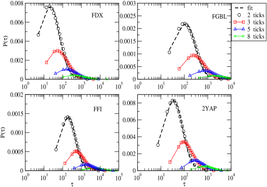
In Fig. 4 we report the first passage distribution obtained by the analysis of our indices at different return levels (expressed in ticks). From the plots it is possible to observe an optimal exit time, $\tau^{\star}$, that is a peak of the first passage distribution, getting longer and longer as the target price difference is increased. Fits of the empirical pdfs with the model of Eq. (2), displayed for a return of 2 ticks, show good qualitative agreements. It is important to stress that what we report is an optimal “exit tick”, rather than time, during business hours. Since the activity of the market is not homogeneous during the day, the optimal horizon should be properly rescaled for practical trading purposes and not used “as it is”.

We notice also that the optimal exit horizon depends on the particular market under consideration, as shown in Fig. 4. Unfortunately, it is not straightforward to identify a relation between $\tau^{\star}$ and some intrinsic properties of the indices, such as the liquidity for example. In fact, the Australian 2YAP, despite being a relatively thin market, has an optimal horizon between the FDX and the FGBL, which are relatively more liquid.

Figure 4: First passage distribution, expressed in tick time, for different markets and target price displacements (in the legend). The height of the peak, as well as $\tau^{\star}$, scale with the target magnitude. For 2 ticks return we also plot the best fit related to the model of Eq. (2).

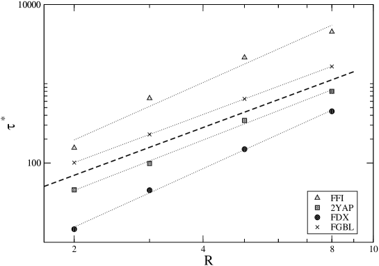
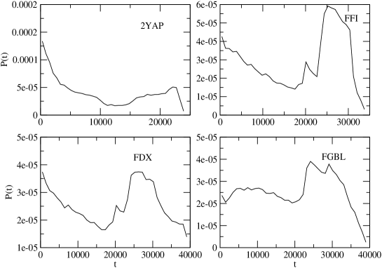
From Fig. 4 we notice also that the shape of the distribution tends to scale with the target price displacement, as expected also for the Brownian walk theory. In particular, we focus our attention on the target dependence, such as the one reported in Eq. (3), of the exit time $\tau^{\star}$. The results are reported on a double logarithmic scale in Fig. 5. Despite the limitations of our temporal frame, that is one trading day, which does not allow to have a particulary broad range of scales available for analysis, a power law relation cannot be rejected by the fits, shown in Fig. 5, where the exponents found are $\gamma\gtrsim 2$ for each index. This result does not match with the ones calculated for regularly spaced samples [19, 20, 22, 23] where $\gamma\lesssim 2$. However, there are very important differences in the investigation lines other that the data sets used. In particular, we consider tick-by-tick data as opposed to evenly sampled and we limit ourselves to a single business day. It is worth pointing out that the values of the exponents found in the present analysis, which would indicate a subdiffusive behaviour for the price moments, have to be considered in the light of the non-homogeneous activity of the market during the day. We refer, in particular, to the series of zero returns that are more likely to be realized during the lunch hours and that can definitely influence the results. To stress this fact, we report in Fig. 6, the distribution of the daily entry times necessary to achieve a return of 5 ticks. As expected, these results closely relate to the daily trading activity with a valley in the middle of the day where the frequency of the data arrival gets lower. Moreover, the distributions of entry times result to be independent on the target tick.

Figure 5: Optimal exit time, $\tau^{\star}$, for the various markets as a function of the target level. The scales are limited by the intra-day analysis that we are carrying on. Nevertheless, a power law, as in Eq. (3), fits quite well the observations (dotted lines). The dashed line is a power law with exponent 2 plotted for visual comparison.

Figure 6: Distribution of entry times for achieving five ticks during a trading day. The distributions, as expected, follow the market activity during business hours. The entry time is reported in seconds from the beginning of the trades.

4 Relaxation times in the limit order book

The study of limit order books has recently attracted the attention of different econophysics groups around the world [24, 25, 26, 27, 28, 29]. Understanding its complex mechanisms implies an understanding of the dynamics of the stock market at a microscopic level, that is, using a metaphor borrowed from physics, an understanding from “first principles”. Far from being so ambitious we investigate the statistical relaxation properties of the aggregated demand and supply for two futures indices: the German DAX (FDX) and the Australian SPI (2YAP). The FDX data are available form 20/07/2004 to 08/12/2006 for a total of $\sim 5\cdot 10^{7}$ samples. Despite the 2YAP data set is one week longer (starting on the 13/07/2004) the number of samples in this case is “just” $\sim 6\cdot 10^{6}$ reflecting a lower frequency of updating. In particular, we refer to relaxation in terms of volume imbalance, $\Sigma$, defined as

$$\Sigma(t)=\sum_{i=1}^{N_{b}}V_{i}^{b}(t)-\sum_{i=1}^{N_{a}}V_{i}^{a}(t),$$ (4)

where $V_{i}^{a,b}$ is the total volume at the $i$th level in the ask ($a$) or bid ($b$) side, $N_{a,b}$ the total number of levels on the respective side of the book and $t$ the tick time. However, the above definition presents a drawback, that is the average order size can differ from market to market and, therefore, the value of $\Sigma$ should be rescaled in order to standardize the results. In order to avoid this inconvenience we use the normalized volume imbalance, $\widehat{\Sigma}$, defined between [-1,1] according to

$$\widehat{\Sigma}(t)=\frac{\sum_{i=1}^{N_{b}}V_{i}^{b}(t)-\sum_{i=1}^{N_{a}}V_{i}^{a}(t)}{\sum_{i=1}^{N_{b}}V_{i}^{b}(t)+\sum_{i=1}^{N_{a}}V_{i}^{a}(t)}.$$ (5)

The relaxation time for a certain threshold volume imbalance $\kappa$ is then defined as

$$\tau(t_{\kappa})={\rm inf}\{T>0\,|\,\widehat{\Sigma}(t_{\kappa}+T)\cdot\widehat{\Sigma}(t_{\kappa})\leq 0\},$$ (6)

given the entry time $t_{\kappa}$, Fig. 7, belonging to the set $\{t_{k}\}$ defined as

$$\{t_{\kappa}\}= \{t>0\,|\,(|\widehat{\Sigma}(t)|-\kappa)\cdot(|\widehat{\Sigma}(t-1)|-\kappa)<0\wedge\cdots$$ (7)

$$(|\widehat{\Sigma}(t)|-\kappa)-(|\widehat{\Sigma}(t-1)|-\kappa)>0\}.$$

In order to simplify the notation, from now on, we use the convention $\left\{\tau_{\kappa}\right\}\equiv\left\{\tau(t_{\kappa})\right\}$.

Figure 7: Propaedeutic plot for the definition of $\tau_{\kappa}$ given a certain threshold ($\kappa=0.7$ in orange). The time series of $\widehat{\Sigma}$ is expressed in tick time. The trade time is calculated by evaluating the number of trades between entry and exit.

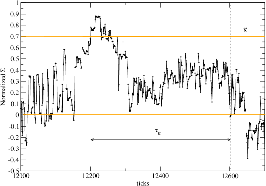
Relaxation times for the order book are very important from both a theoretical point of view and for the purposes of technical trading. In the first case a proper investigation would be able shed some light on the dynamical behaviour which characterize the traders reaction to a particular condition of the market, that is when there is imbalance between demand and supply. This “out-of-equilibrium” condition can be, in principle, very different from the situation when the book is balanced: the question is, how do the market participants act to drive the market to a new (meta-stable) “equilibrium”? In the context of technical trading, relaxation times could be used to determine temporal thresholds for the closure of a trade that was conditioned to a certain book configuration.

Figure 8: Probability distribution function, for FDX, of relaxation times, $\tau_{\kappa}$, expressed in trades, for different $\kappa$ values. In the inset we show the fit, for $\widehat{\Sigma}=0.4$, against the stretched exponential of Eq. (8). This distribution provides a very good description of the empirical pdf. The dashed line, instead, is a power law displayed for visual comparison.

Figure 9: Same plot as Fig. 8 but for the 2YAP. Also in this case the stretched exponential fit, shown in the inset, seems to provide a good model for the distribution of relaxation times.

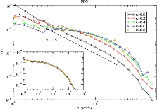
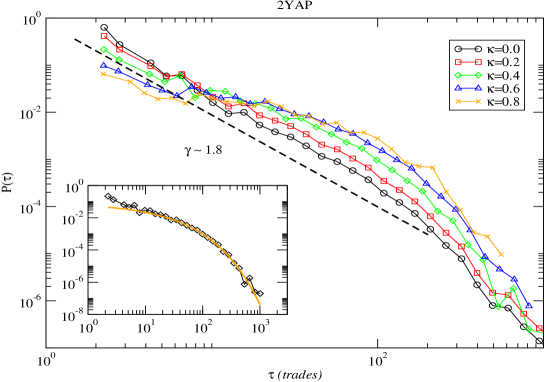
In Figs. 8 and 9, respectively for the FDX and 2YAP, we report the empirical probability distribution functions (pdfs), $P$, of the relaxation times, $\tau_{\kappa}$ for various thresholds $\kappa$ of the normalized volume imbalance. From these plots we can infer a clear correlation between the shape of the distribution and the threshold imbalance: as we move from large to small $\kappa$s the pdfs change in an almost continuous fashion. Moreover, we find that over almost all the range of $\kappa$ under examination the distributions are very well described by a stretched exponential,

$$P(\tau)\propto{\rm e}^{-\left(\frac{\tau}{\tilde{\tau}}\right)^{\alpha}},$$ (8)

where $\tilde{\tau}$ is the characteristic time scale and the exponent $\alpha$ belongs to the interval (0,1] . The insets of Figs. 8 and 9 report the fits for $\kappa=0.4$. These findings share interesting similarities with relaxations in solid state physics [31, 33, 34] where it has been shown that different models can explain the rise of stretched exponential distributions. In particular, the convolution of Poisson processes with different characteristic times seems to be one of the most plausible scenarios [35, 31]. In the continuous limit, we can formalize this concept through the the Kohlrausch-Williams-Watts equation (KWW),

$${\rm e}^{-\left(\frac{\tau}{\tilde{\tau}}\right)^{\alpha}}=\int_{0}^{\infty}{\rm e}^{-\frac{\tau}{\tau^{\prime}}}\,\rho(\tau^{\prime})\,d\tau^{\prime}$$ (9)

where $\rho(\tau^{\prime})$ is the distribution of independent time scales, or Debye distribution, and can be calculated numerically for a fixed value of $\alpha$ [31]. The parameters of the stretched exponential, therefore, are related to the specific form of the Debye distribution. Despite its intuitive interpretation, this framework presents a drawback. In fact, assuming that Eq.(9) holds, we have to postulate the existence of a class of Debye distributions that can justify the ubiquity of stretched exponential relaxations. This issue can be partially solved by realizing that a L$\acute{\rm e}$vy stable distribution $L_{\alpha,\beta}$ with parameters $\alpha\in(0,1)$ and $\beta=-1$ is a solution of Eq. (9) [39]. The parameters characterize, respectively, the “fatness” of the distribution’s tails and the degree of asymmetry and, therefore, $\beta=-1$ corresponds to a positively defined support for $L_{\alpha,\beta}$. The strength of this framework relies on the fact that L$\acute{\rm e}$vy distributions are attractors in the distributions space and, therefore, the appearance of a stretched exponential would be justified in the standard framework of stochastic processes [39]. In particular, L$\acute{\rm e}$vy distributions are fixed points for the addition of i.i.d. random variables, $x_{i}$, whose individual distributions are asymptotically a power law, $P_{i}(x_{i})\sim|x_{i}|^{-1-\nu}$ with $0<\nu<2$, that is, with infinite variance.

Coming back to the relaxation times observed for the volume imbalance, Figs. 8 and 9, and given the previously mentioned conditions for the appearance of L$\acute{\rm e}$vy distributions, we can argue that such an attractor for $\rho(\tau^{\prime})$ in Eq.(9) can result as a consequence of the “fat” tails intrinsic in the human activity [40, 41, 42] and, therefore, help justify the empirical results. However, we still have to understand how the changes in $\rho$ are related to the changes in $\kappa$. One possible scenario involves the set of “herding effects” [43, 44]. In this case, as the imbalance in the book increases (hence $|\kappa|>0$), well informed individuals and institutions (here, those with knowledge of the instantaneous order book state) invoke order submission and cancellation strategies that are more adapted to the large observed imbalance - for example, strategies that require longer waiting times between limit order submission and cancellation, or the submission of limit orders further from the current mid point price. Thus, as the informed market participants tend towards a broadly similar set of strategies, the heterogeneity within the market is reduced, leading to changes in the Debye distribution of order arrival and cancellation waiting times and, eventually, to changes in the distribution of imbalance relaxation times. Of course this scenario is speculative and it would be important to back up these qualitative arguments with rigorous numerical simulations. Moreover, numerical calculations of Debye distributions could help to shed some light on this issue.

For $\kappa\sim 0$ the situation is slightly different. In this regime the distributions become so stretched that a power law, $P(\tau)\propto\tau^{-\gamma}$, provides a better description of them in terms of least squared error. The change in the shape of the distributions, from stretched exponential towards a power law can still be interpreted in the framework of Eq. (9) given that the convolution of exponentials can give rise to asymptotic power laws [45]. More intuitively, we can interpret this “near-equilibrium” state in terms of diffusion processes. In fact, without any extra information given by the difference in demand and supply new limit orders are distributed on each side of the book according to a large number of heterogeneous strategies based on other indicators. This phase implies a diffusion process for the variable $\Sigma$ (or $\widehat{\Sigma}$) and the appearance of power law relaxation times identified with a problem of first return to the origin [45]. In this framework, for a fractional Brownian motion it has been analytically shown that the asymptotic pdf of waiting times between two consecutive crossings of the origin would be a power law with exponent, ${H-2}$ where $H$ is the Hurst parameter of the walker [9]. Note that for the simple Brownian motion $H=0.5$ and, therefore, the asymptotic power law exponent would be $\gamma=1.5$ [8, 9, 10]. For the time series under examination the exponent of the power law estimated for small imbalances, $\kappa\sim 0$, is $\gamma\sim 1.5$ for the FDX and $\gamma\sim 1.8$ for the 2YAP. A dashed line for visual guidance is reported in Figs. 8 and 9. The difference in the two exponents can be justified, at least, by two factors: difference in liquidity (the FDX is more liquid compared to the 2YAP and, as a consequence, its behaviour is closer to that of a random walk) and lack of information for the 2YAP (we have just 5 levels on each size of the book and more information may be “hidden” at deeper levels).

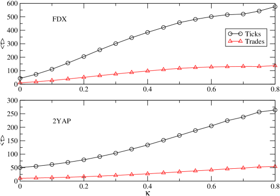
As a final note, we report in Fig. 10 the estimate of mean relaxation times as a function of $\kappa$ in both trade time and tick time. For $0.1\lesssim\kappa\lesssim 0.6$, the increase of the mean relaxation time is a linear fiction of $\kappa$ and, given that for a stretched exponential distribution the average relaxation time is given by

$$\langle\tau\rangle=\frac{\tilde{\tau}}{\alpha}\Gamma\left(\frac{1}{\alpha}\right),$$ (10)

then we can infer that, in this regime, $\tilde{\tau}/\alpha\propto\kappa$.

Figure 10: Mean relaxation times expressed in trades and ticks for the FDX (top) and 2YAP (bottom). In the mid range of imbalances, the increase of the average price can be well described by a linear function of $\kappa$.

5 Conclusion

This work has focussed on demonstrating the application of a range of physical methods to high-frequency and tick-by-tick financial time series. The results presented relate to the local time-varying scaling properties of the price time series, the distribution of the so-called optimal investment horizon and also to the relaxation properties of disequilibrium limit order books.

In section 2 we demonstrated the use of the concept of local Hurst exponent in order to investigate the short scale dynamical properties of the correlations in different futures contracts (indices, commodities, exchange rate and fixed income) from the beginning of 2003 to the end of 2004.

Analysis of the behaviour of $H_{L}(t)$ at different scales, and in particular its distribution, points out a scale dependent and non-stationary evolution of this scaling exponent, independent of the specific kind of contract. The Eurex Bunds, BOBL and U.S Treasury Bonds, for example, display an average persistent behaviour over time scales of approximately three weeks but they then become antipersistent, on average, for time scales of the order of one day. Moreover, we observe changes in the shape of the pdfs of $H_{L}(t)$ with time. This fact points to the existence of different market phases in the two years period from 1/1/2003 to 31/12/2004 and, therefore, evidence for non-stationarity. These empirical facts are in contrast with the EMH hypothesis, according to which $H_{L}(t)$ should be constant and equal to 0.5 for each time scale. It is worth to stress that the dynamical behaviour of the Hurst exponent is not related only to the liquidity of the market but also to the variety of time horizons involved in the trade of a particular asset. As a consequence, markets which involve many exogenous agents, such as the S&P500, tend to be more “efficient”. A point we would like to emphasise is that the concept of Hurst exponent for non-stationary time series has a practical validity only in the period and the scale of observation. By estimating $H$ with a large sample, due to the coarse-grain procedure of the DFA algorithm, we lose the local information and we obtain an “average” value over that period. This can or cannot be a problem for technical trading: it depends on the horizon we are interested in.

In section 3 we have shown the existence of an optimal exit time, or more correctly “exit tick”, necessary to achieve a pre-fixed return. Moreover, even if on a limited range, the scaling of this quantity with the target tick can be well approximated with a power law with exponent $\gamma\gtrsim 2$ depending on the market under consideration. Previous studies have revealed a similar qualitative behaviour but with significant discrepancies in the scaling index value [19, 20, 22, 23]. The discrepancies can be taken into account by the tick nature of our data and the restriction of our analysis to business hours. To the best of our knowledge it is the first time that the optimal exit horizon has been calculated at tick-by-tick frequency inside a trading day. From the practitioner point of view the existence of such a stylized fact can potentially be exploited but its value has to be taken with care. In fact, the tick frequency depends on the intra-day pattern activity of the market and, therefore, the estimated value of $\tau^{\star}$. Note the usage of real time, that is sampling at a regular frequency, will lead to similar problems.

In section 4 we reported on investigations into the dynamical properties of the order book conditioned to an imbalance in the aggregated demand/supply. In particular, we focus on the time required for the order book to reach a new (meta-stable) “equilibrium”. To the best of our knowledge this is the first investigation of this kind. Empirical results show how the relaxation times behave in a way that is analogous to that found in certain physical systems. In particular, the distribution $P(\tau_{\kappa})$ seems to have a relatively broad spectrum that can be very well described by a stretched exponential distribution with characteristic parameters that depend on the threshold imbalance. This dependence can be related to a decrease in the heterogeneity of trader strategies as we move towards larger imbalances in the book, for example, due to herding mechanisms. For small initial imbalances, instead, diffusion processes seem to dominate the dynamics of the book.

In conclusion, we have shown that methods of physical analysis produce useful and potentially valuable insights into the dynamics of market microstructure. A feature of the results presented in this work is that they would not have been obtained without access to a high-frequency or tick-by-tick record of both market trade data and the limit order book state. We note that econophysicists and market practitioners are increasingly turning to the study of market microstructure, with the aim of gaining a better understanding of the complex system that is the financial marketplace. Still, questions on items such the source of market inefficiencies and the nature of the complex interplay between the limit order book, price evolution and order flow remain largely unaddressed. It is for these reasons that we expect to see the types of methods and time series discussed in this work to begin to feature ever more prominently in future econophysics literature.

References

- [1] J.-P. Bouchaud and M. Potters, Theory of financial risk, Cambridge University Press, Cambridge, 1999.
- [2] R. N. Mantegna and H. E. Stanley, An introduction to econophysics: correlation and complexity in finance, Cambridge University Press, Cambridge, 1999.
- [3] J. Voit, The Statistical Mechanics of Financial Markets, Spriger-Verlag, Berlin, 2005.
- [4] J. Feder, Fractals, Plenum Press, New York, 1998.
- [5] M. M. Dacorogna, R. Gençay, U. Müller, R. B. Olsen, and O. V. Pictet, An introduction to high-frequency finance, Academic Press, San Diego, 2001.
- [6] M. H. Jensen, “Multiscaling and structure functions in turbulence: An alternative approach,” Phys. Rev. Lett. 83, pp. 76–79, Jul 1999.
- [7] L. Biferale, M. Cencini, D. Vergni, and A. Vulpiani, “Exit time of turbulent signals: A way to detect the intermediate dissipative range,” Phys. Rev. E 60, pp. R6295–R6298, Dec 1999.
- [8] G. Grimmett and D. Stirzaker, Probability and Random Processes, Oxford University Press, New York, 1994.
- [9] M. Ding and W. Yang, “Distribution of first return time in fractional Brownian motion and its application to the study of on-off intermittency,” Physical Review E 52, p. 207, 1995.
- [10] G. Rangarajan and M. Ding, “First passage time distribution for anomalous diffusion,” Physics Letters A 273, pp. 322–330, 2000.
- [11] M. Bartolozzi, C. Mellen, T. Di Matteo, and T. Aste, “Multi-scale correlations in different futures markets,” The European Physical Journal B 58(2), pp. 207–220, 2007.
- [12] C.-K. Peng, S. V. Buldyrev, S. Havlin, M. Simons, H. E. Stanley, and A. L. Goldberger, “Mosaic organization of DNA nucleotides,” Physical Review E 49, pp. 1685–1689, Feb 1994.
- [13] R. L. Costa and G. L. Vasconcelos, “Long-range correlations and nonstationarity in the Brazilian stock market,” Physica A 329, p. 231, 2003.
- [14] T. Di Matteo, T. Aste, and M. M. Dacorogna, “Scaling behaviors in differently developed markets,” Physica A 324, p. 183, 2003.
- [15] D. O. Cajueiro and M. B. Tabak, “The Hurst exponent over time: testing the assertion that emerging markets are becoming more efficient,” Physica A 336, p. 231, 2004.
- [16] T. Di Matteo, T. Aste, and M. M. Dacorogna, “Long term memories of developed and emerging markets: using the scaling analysis to characterize their stage of development,” Journal of Banking & Finance 29, p. 827, 2005.
- [17] R. Liu, T. Di Matteo, and T. Aste, “True and apparent scaling: The proximities of the Markov-switching multifractal model to long-range dependence,” Physica A 383, p. 35, 2007.
- [18] T. Di Matteo, “Multi-scaling in finance,” Quantitative Finance 7(1), p. 21, 2007.
- [19] I. Simonsen, M. H. Jensen, and A. Johansen, “Optimal investment horizon,” The European Physical Journal B 27, pp. 583–586, 2002.
- [20] M. H. Jensen, A. Johansen, and I. Simonsen, “Inverse statistics in economics: the gain-loss asymmetry,” Physica A 324, p. 338, 2003.
- [21] M. H. Jensen, A. Johansen, F. Petroni, and I. Simonsen, “Inverse statistics in the foreign exchange market,” Physica A 340, p. 678, 2004.
- [22] W.-X. Zhou and W.-K. Yuan, “Inverse statistics in stock markets: universality and idiosyncracy,” Physica A 353, p. 423, 2005.
- [23] K. Karpio, M. A. Zaluska -Kotur, and A. Orlowski, “Gain-loss asymmetry for emerging stock markets,” Physica A 375, p. 599, 2007.
- [24] J. D. Farmer, L. Gillemot, F. Lillo, S. Mike, and A. Sen, “What really causes large price changes?,” Quantitative Finance 4(4), pp. 383–397, 2004.
- [25] F. Lillo and M. J. D. Farmer, “Long memory of the efficient market,” Nonlinear Dynamics and Econometrics 8(3), p. 1, 2004.
- [26] F. Lillo and J. D. Farmer, “The key role of liquidity fluctuations in determining the large price changes,” Fluctuations and noise letters 5(2), p. L209, 2005.
- [27] P. Weber and B. Rosenow, “Order book approach to price impact,” Quantitative Finance 5(4), p. 357, 2005.
- [28] P. Weber and B. Rosenow, “Large stock price changes: volume or liquidity?,” Quantitative Finance 6(1), p. 7, 2006.
- [29] M. Wyart, J.-P. Bouchaud, J. Kockelkoren, M. Potters, and M. Vettorazzo, “Relation between bid-ask spread, impact and volatility in double auction market,” preprint: physics/0603084 , 2006.
- [30] C. Cao, O. Hansch, and X. Wang, “The informational content of an open limit order book,” Working paper Pennsylvania State University , 2003.
- [31] F. Alvarez, A. Alegria, and J. Colmenero, “Relationship between the time-domain Kohlrausch-Williams-Watts and frequncy-domain havriliak-negami relaxation function,” Physical Review B 44, p. 7306, 1991.
- [32] J.-P. Bouchaud, M. Mzard, and M. Potters, “Statistical properties of stock order books: empirical results and models,” Quantitative Finance 2(4), pp. 251 – 256, 2002.
- [33] K. Weron and M. Kotulski, “On the Cole-Cole relaxation function and related Mittag-Leffler distribution,” Physica A 232, pp. 180–188, 1996.
- [34] M. Magdziarz and K. Weron, “Anomalous diffusion schemes underlying the Cole-Cole relaxation: the role of the inverse-time -stable subordinator,” Physica A 367, pp. 1–6, 2006.
- [35] J. Klafter and M. F. Shlesinger, “On the relationship among three theories of relaxation in disordered systems,” Proceedings of the National Academy of Sciences USA 83, pp. 848–851, 1986.
- [36] B. Castaing, Y. Gagne, and E. J. Hopfinger, “Velocity probability density functions of high Reynolds number turbulence,” Phys. D 46(2), pp. 177–200, 1990.
- [37] C. Beck, “Superstatistics,” Physica A 322, p. 267, 2003.
- [38] J. Honerkamp, Statistical physics: an advanced approach with applications, Springer-Verlag, Berlin, 1998.
- [39] W. Paul and J. Baschnagel, Stochastic processes: from physics to finance, Springer, Berlin, 1999.
- [40] A.-L. Barabsi, “The origin of bursts and heavy tails in human activity,” Nature 435, p. 207, 2005.
- [41] M. Bartolozzi, D. B. Leinweber, and A. W. Thomas, “Stochastic opinion formation in scale-free networks,” Physical Review E 72, p. 046113, 2005.
- [42] K.-I. Goh and A.-L. Barabsi, “Burstiness and memory in complex systems,” preprint: physics/0610233 , 2006.
- [43] R. Cont and J.-P. Bouchaud, “Herd behaviour and aggregate fluctuations in financial markets,” Macroeconomics Dynamics 4, p. 170, 2000.
- [44] M. Bartolozzi and A. W. Thomas, “Stochastic cellular automata model for stock market dynamics,” Physical Review E 69, p. 046112, 2004.
- [45] D. Sornette, Critical phenomena in natural sciences, Springer-Verlag, Berlin, 2004.