Random walk on a population of random walkers

Abstract

We consider a population of $N$ labeled random walkers moving on a substrate, and an excitation jumping among the walkers upon contact. The label $\mathcal{X}(t)$ of the walker carrying the excitation at time $t$ can be viewed as a stochastic process, where the transition probabilities are a stochastic process themselves. Upon mapping onto two simpler processes, the quantities characterizing $\mathcal{X}(t)$ can be calculated in the limit of long times and low walkers density. The results are compared with numerical simulations. Several different topologies for the substrate underlying diffusion are considered.

1 Introduction

A general stochastic process $\xi(t)$ can be viewed as the time evolution of one (or more) random variable [1], the particular dependence on $t$ of the transition probabilities between the states giving rise to different models. Among the most widely studied stochastic processes in physics are Markov processes, where the transition probabilities at $t_{1}>t$ depend only on $\xi(t)$ and $t$, and not on the previous history of the system. In the simplest case the time parameter $t$ is discrete, and $\xi(t)$ is called a Markov chain; the case of a Markov chain with transition probabilities independent of $t$ is by far the most studied. If the transition probabilities in the time interval $(t_{0},\,t_{0}+t)$ do depend on $t$ (with a given distribution function), but not on $t_{0}$, we have homogeneous processes. Depending on the particular functional dependence on $t$, we can obtain Poisson processes, Wiener processes, and so on. Relaxing the homogeneity property, we can obtain the inhomogeneous version of the previous processes.

Much more general assumptions on the time-dependence of the transition probabilities can be given, but the resulting models are rarely explicitly solvable. In this paper we define and solve a particular discrete-time stochastic process: its transition probabilities are a stochastic process themselves.

The process we consider is a “second-level” random walk, or random walk on random walkers. We consider $N$ labeled random walkers, diffusing on a given substrate. Such random walkers can define a dynamic meta-graph: each random walk is seen as a node of the meta-graph and a link between two of them is drawn whenever they are within a distance $R$ on the substrate. Then, we study the diffusion of a “second-level” random walk on such meta-graph.
Apart from its mathematical interest, this kind of system is also able to model a diffusion-reaction process. In fact, each walker diffusing on the substrate represents a particle (all particles belonging to the same chemical species) that can be either in an excited ($A^{*}$) or in an unexcited ($A$) state, the former corresponding to the node carrying the second-level random walker. When an excited particle meets an unexcited one, they immediately react according to the scheme

$$A^{*}+A\rightarrow A+A^{*}.$$ (1)

This reaction mechanism is known as homogeneous energy transfer (ET) which takes place from an excited molecule [donor (A*)] to another unexcited molecule [acceptor (A)], according to the scheme (1). This process stems from Coulombic (long-range [2]) and exchange (non-radiative, short-range [3]) interactions amongst the particles. If we just focus on the energy transfer via exchange (under the implicit assumption that the relaxation takes zero time), this allows to restrict transfer interaction to nearest-neighbour particles only.

If we define an abstract space whose points are the $N$ random walkers, the excitation transfer corresponds to a stochastic process $\mathcal{X}(t)$ on the points of this space; hence, to a “second-level” random walk. The transition probabilities of this process depend on the relative positions of the random walkers, hence they are a stochastic process themselves. It is possible to show how the process $\mathcal{X}(t)$ can be mapped exactly onto simpler processes, involving $N$ or $N-1$ simple random walkers on the same lattice; the study of the excitation jumps is here mapped on the study of the passage times of these walkers through the origin. These simpler processes can be solved in the limit of large times and low walkers densities.

The paper is organized as follows. In Sec. 2 we describe the model; in Sec. 3 we provide two mappings to simpler processes that allow us to obtain the asymptotic behaviour of the quantities of $\mathcal{X}(t)$. In Sec. 4 these results are compared with numerical simulations. Sec. 5 contains our conclusions and perspectives.

2 The model

We consider $N$ regular random walkers, labeled with the numbers from 1 to $N$, moving on a finite structure (henceforth, the substrate). The position of the $i$th walker at time $t$ is $x_{i}(t)$; at time 0 all the positions are random. At $t=0$ one of the walkers, $i_{0}$, carries an excitation; we assume without loss of generality that $i_{0}=1$.

The following usual quantities for random walks on lattices will be useful. For a walker starting from $r$ at time 0, we define the probability $P_{0}(r,\,t)$ of being at 0 at time $t$, and the probability $F_{0}(r,\,t)$ of being at 0 for the first time at time $t$. We also define their generating functions, $\tilde{P}_{0}(r,\,\lambda)=\sum_{t=0}^{\infty}P_{0}(r,\,t)\lambda^{t}$ and $\tilde{F}_{0}(r,\,\lambda)=\sum_{t=1}^{\infty}F_{0}(r,\,t)\lambda^{t}$.

We fix a collision radius $R\geq 0$: at time $t$ two walkers meet (or collide) if their distance on the lattice is $\leq R$. In this paper we consider $R=1$ but there are no substantial differences for different $R$ (the choice $R=0$ is here neglected to avoid parity effects, and used for explanations only in Sec. 3). When the walker $i$ carrying the excitation collides with another walker $j$, the excitation jumps from $i$ to $j$. If it collides with more than one walker at the same time (which we will call a multiple hit), the excitation jumps on one of them chosen randomly.

The model just described defines a discrete-time stochastic process $\mathcal{X}(t)$, where the state space of the system is composed by the set of the random walkers. At time $t$ the system is in state $i$ if the excitation is on walker $i$

Formally, the process is defined by the state space

• $\mathcal{X}(t)\in\mathcal{N},\mathcal{N}=\{1,2,\ldots,N\}$;

by the initial condition:

• $\mathcal{X}(0)=1$;

and the evolution rule:

• let $\mathcal{X}(t)=i$; consider the set $\mathcal{C}=\{j:\|x_{i}(t)-x_{j}(t)\|\leq R;\,j\neq i\}$ .
  If $\mathcal{C}=\varnothing$, then $\mathcal{X}(t+1)=i$.
  If $\mathcal{C}\neq\varnothing$, then $\mathcal{X}(t+1)=j$, where $j$ is chosen randomly among the elements of $\mathcal{C}$ with equal probability.

Here, the transition (or jump) probabilities, given by the evolution rule, are a stochastic process. In particular, at time $t$ the transition probability from state $i$ ($\mathcal{X}(t)=i$) to state $j$ ($\mathcal{X}(t+1)=j$) is a function of the positions $x_{i}(t)$ and $x_{j}(t)$ of the two RWs, hence a function of two stochastic processes.

Several quantities can be defined for $\mathcal{X}(t)$, much in the same way as for regular random walks on a lattice. We define:

• $\mathcal{J}(t)$, the average number of jumps performed by the system up to time $t$; the probability $\mathcal{J}(t,\,h)$ that the number of jumps performed by the system is $h$ at time $t$, $\mathcal{J}(t)=\sum_{k=1}^{N}k\mathcal{J}(t,k)$.

• $\mathcal{S}(t)$, the average number of different states visited at time $t$; the probability $\mathcal{S}(t,k)$ that $k$ different states have been visited by the system at time $t$, $\mathcal{S}(t)=\sum_{k=1}^{N}k\mathcal{S}(t,k)$.

• the Cover Time $\tau$, defined as the average time required to visit all the $N$ walkers (analogous to the lattice-covering time for random walks [7]). We also define $\pi$ as the average number of jumps required to visit all the states ($\pi\leq\tau$).

The substrates considered will be Euclidean (hypercubic) lattices of linear size $L$ and volume $L^{d}$ (with $d=1,\,2,\,3$), endowed with periodic boundary conditions.

We also will consider fractal substrates. It is well known [4, 5] that fractals are described by at least two different dimensional parameters. One is the fractal dimension $d_{F}$, describing the large-scale dependence of the volume (or mass) $V(r)$ of the structure on the distance $r$ from a point 0 chosen as the origin: $V_{0}(r)\sim a_{0}r^{d_{F}}$ (here and in the following lines, $a_{0}$, $b_{0}$ and $c_{0}$ are constants depending on the point 0). The other is the spectral, or connectivity, dimension $d_{s}$, describing the long-time behaviour of diffusive phenomena on the fractal. For example, for $t\rightarrow\infty$ the probability of return to the starting point for a RW on the fractal is $P_{0}(t)\sim b_{0}t^{-d_{s}/2}$, and the average number of different sites visited by the RW is $S(t)\sim c_{0}t^{\min(d_{s}/2,\,1)}$. For Euclidean lattices, $d_{s}=d_{F}=d$. In a lattice (either Euclidean or fractal) with $d_{s}\leq 2$ a random walker starting from a point 0 is bound to return to 0 an infinite number of times with probability 1, and the lattice is called recurrent. For $d_{s}>2$, the walker has a non-null probability to escape to infinity without returning to 0, and the lattice is called transient.

The fractal lattices we will consider (fig. 1) are Sierpinski gaskets of linear size $L$ and volume $L^{\log 3/\log 2}$ ($d_{F}=\log 3/\log 2$). Their spectral dimension is $d_{s}=2\log 3/\log 5$ (hence, they are recurrent: $d_{s}<2$) .

Figure 1: Sierpinski gasket.

All the quantities we are interested in will be examined as functions of $N$ and $L$.

3 Analytical Results

The purpose of this section is to show how our model can be mapped onto two different, and easier, models, that we shall call picture 1 and 2 respectively. In these two pictures, and in the low-density (LD) limit (when multiple hits are negligible), the asymptotic behaviour of the quantities of the previous section can be found.

Let us take figure 2 as a reference. The upper part of the figure exemplifies the basic process. At $t=0$ the excitation is on walker 1 (the system in state 1); at $t_{1}$ walker 2 hits walker 1 and the excitation jumps on walker 2 (the system jumps on state 2). At times $t_{2}$ and $t_{3}$ the excitation jumps on walker 3 and then on walker 1 again. This can be summarized by introducing the sequence of jumping times

$$0,\,t_{1},\,t_{2},\,t_{3},\,\ldots$$ (2)

and the sequence of visited states

$$0,\,i_{1},\,i_{2},\,i_{3},\,\ldots$$ (3)

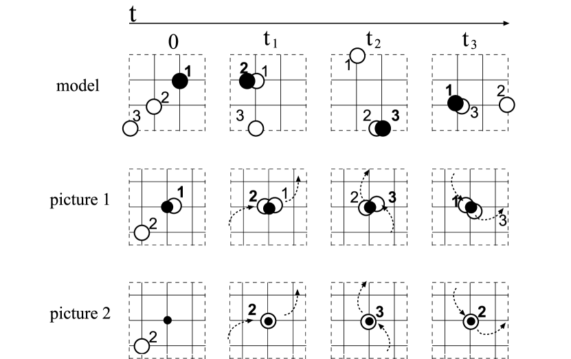
Figure 2: Top: the original process on a square lattice at four nonconsecutive times 0, $t_{1}$, $t_{2}$, $t_{3}$. The walker carrying the excitation is the black circle. The excitation jumps from $1$ to $2$ at time $t_{1}$, from $2$ to $3$ at time $t_{2}$, and from 3 to 1 at time $t_{3}$. Middle: picture 1. The same process in the reference frame of the excitation (small black circle fixed at the origin). The walkers are stuck at the origin when carrying the excitation in the original model, and get free when the excitation jumps to another walker. The jumping times are the same. Bottom: picture 2. Here, the black circle marks the origin. The associated free process, with $N-1$ random walkers labeled with the numbers from 2 to $N$, is shown. Picture 1 is obtained as follows. We start from the ordering $(1,\,2,\,3)$. Each time walker $i$ of the associated process crosses the origin, it exchanges its label with the previous walker that crossed it, starting from walker 1; alternatively spelled, walkers at position 1 and $i$ of the present ordering exchange their labels. Hence, 2 crosses the origin at time $t_{1}$ and exchanges its label with 1; the new ordering is $(2,\,1,\,3)$; 3 crosses the origin at time $t_{2}$ and exchanges the label with 2; the new ordering is $(3,\,1,\,2)$. Finally, 2 crosses the origin at time $t_{3}$; the walkers at positions 2 and 1 exchange their labels: the new ordering is $(1,\,3,\,2)$.

Picture 1 (stuck-and-free picture) We consider the process in the reference frame of the excitation. In this frame, the walker carrying the excitation is stuck at the origin, and the other $N-1$ walkers perform a regular random walk, with 2 jumps on each time step. Here, the jump of the excitation from walker $i$ to walker $j$ corresponds to the following: walker $j$ hits the origin and gets stuck, while walker $i$ gets free and starts performing its own RW.

In this picture, the process is a double-state RW process [8], because each walker can exist in two different states: either stuck at the origin or free. When a walker is free, this picture allows us to use well-known quantities from random-walk theory: for example, the probability for walker $i$, starting from $r_{i}$ at time 0, of getting stuck at the origin at time $t$ is (neglecting multiple hits) $F_{0}(r_{i}-r_{0},\,2\,t)$. This problem is still completely described by the above sequences of times (2) and states (3).

We remark that this mapping is possible only for translationally invariant (Euclidean) lattices, where the lattice in the reference frame of the excitation is the same as the original one. It is not possible for fractal lattices; this will be clarified below.

Picture 2 (label permutation picture)

When walker $2$ hits walker $1$ at the origin and gets stuck (picture 1), the random walk subsequently performed by $1$ is just the random walk that would have been performed by $2$ if no sticking effect had existed: that is, if walkers $1$ and $2$ simply had switched their labels without changing their state. This label switch can be seen as the action of a transposition $(1\;2)$ of the numbers 1 and 2 on the sequence $\mathcal{N}$.

Consider the process (let us call it the associated free process) with $N-1$ free RWs, labeled from 2 to $N$, on the same lattice, and walker 1 stuck once and for all at the origin. The process in picture 1 is the same as the associated free process, plus the following condition: when a walker hits the origin it switches its label with the last walker that has hit the origin before it (with the condition that the first walker has been 1). In general, when walker $i$ of the associated free process hits the origin, a permutation $\Pi=(1\;i)$ of elements $1$ and $i$ is induced on the original sequence $\mathcal{N}$ (since the last stuck walker is always at the first place in the permutated sequence).

The sequence of jump times (2) hence is equal to the sequence of crossing times of $N-1$ random walkers through the origin. Hence, the sequence of the walkers that cross the origin in the associated free process

$$0,\,j_{1},\,j_{2},\,j_{3},\,\ldots,$$

is related to the sequence for the original process by

$$i_{1}=(\Pi_{1}\mathcal{N})_{j_{1}};\,\,i_{2}=(\Pi_{2}\mathcal{N})_{j_{2}};\,\,i_{3}=(\Pi_{3}\mathcal{N})_{j_{3}};\,\ldots$$

where $\Pi_{1}=(1\;j_{1})$; $\,\Pi_{2}=(1\;j_{1})(1\;j_{2})$; $\,\Pi_{3}=(1\;j_{1})(1\;j_{2})(1\;j_{3})$, and so on.

Two observations are necessary at this point. First: both pictures are valid only for translationally invariant lattices; for fractals, for example, the lattice in the frame of reference of the excitation does not coincide with the original one (indeed, it is not even fixed but changes with $t$). However, several of our numerical results suggest that the asymptotic results derived in the euclidean case also hold (in some averaged sense) for non-integer-dimensional cases. This point will be stressed again case by case.

Second: we depicted pictures 1 and 2 for a model with null range $R=0$, while most of our numerical result concern the case $R\neq 0$ (mostly $R=1$), chosen to avoid the parity effects (since most of our lattices are bipartite graphs, walkers starting from the “wrong” sites would never meet). A non-null range in the original model corresponds to a sticking area greater than the origin in picture 1, and to the passage to a region greater than the origin in picture 2. This means that in picture 1 and 2 the walkers can perform jumps to the origin even when the origin is not a nearest-neighbor site. We expect, however, that the existence of a non-null range will only result in a rescaling of the asymptotic laws (usually by a factor $v/V$, where $v$ is the discrete volume of the region). We will stress this point in the analytic results where necessary.

3.1 Number of jumps for large times

This quantity is easily calculated in picture 2. If we consider low-density systems, that is, we neglect the probability of multiple hits of the origin by the walkers, the number of jumps at time $t$ is the number of passages through the origin made by $N-1$ RWs at time $t$, that is $N-1$ times the number of passages through the origin made by a single RW. The mean number of times that a RW starting from $r$ visits the origin in a walk of $t$ steps is independent of $r$ for large $t$, and equals $\sim\frac{t}{V}$, where $V$ is the volume of the lattice [9]. The average number of jumps is given by the mean number of times that $N-1$ independent RWs hit the origin, that is

$$\mathcal{J}(t)\sim\frac{N-1}{V}t,$$ (4)

neglecting multiple hits. In the case of walkers with non-null radius of action we must consider a finite-size trap. If $v$ is the volume of the trap, the result is

$$\mathcal{J}(t)\sim\frac{(N-1)\,v}{V}t.$$ (5)

For example, for a radius $R=1$ we have $v=2d+1$ for hypercubic lattices of dimension $d$.

For $\mathcal{J}(h,t)$ (the probability that the number of passages performed by the excitation is $h$ at time $t$) no analytical results are known, and we will rely only on numerical simulations.

3.2 Cover Time

The Cover Time is defined as the average time needed for the system to visit all the states. In the LD limit this is equal (looking at picture 2) to the time needed for $N-1$ different walkers to be absorbed into a trap located at the origin. This is a many-body problem (already formulated in the frame of extreme value statistics, see e.g. [6]), and its exact solution is not yet known.

We will adopt here an approximation. We recall that $F_{0}(r,\,t)$ is the probability density for the first-passage time to the origin of a walker starting from $r$. We know that on hypercubic lattices the average first passage time for a RW through the origin, averaged over all possible starting positions, is

$$\langle t\rangle_{V}=\sum_{r}\frac{1}{V}\sum_{t=0}^{\infty}tF_{0}(r,t)\sim a_{d}\,g_{d}(V),$$

where the approximation is valid for $V$ large; $a_{d}$ is a constant that depends only on $d$, and $g_{d}(V)$ is the volume-depending part:

$$g_{d}(V)=\left\{\begin{array}[]{cc}V^{2}&d=1\\ V\,\log V&d=2\\ V&d>2\end{array}\right.$$

In the case of fractal lattices, the general formula $\langle t\rangle_{V}\sim a_{d_{s}}\,g_{{d_{s}}}(V)$ can be heuristically justified, and has been calculated analitically in two particular cases [10, 11]; here,

$$g_{{d_{s}}}(V)=\left\{\begin{array}[]{cc}V^{2/d_{s}}&d_{s}<2\\ V\,\log V&d_{s}=2\\ V&d_{s}>2,\end{array}\right.$$

$d_{s}$ being the spectral dimension of the lattice.

Our approximation consists in assuming that the first passage time of the first out of $m$ RWs is that of one RW divided by $m$. Hence, the time of absorption of the first walker is $g_{d}(V)/(N-1)$, that of the second walker (the first out of $N-2$ left) is $g_{d}(V)/(N-2)$ and so on. The Cover Time is:

$$\tau(N,V)\sim\displaystyle\sum_{n=1}^{N-1}\frac{a_{d}\,g_{d}(V)}{N-n}\sim\left[\gamma+\log N+O(N^{-1})\right]\,a_{d}\,g_{d}(V),$$ (6)

where the last relation holds in the limit of large $N$.

From what said before, we can easily estimate the average number of jumps required to visit all the states:

$$\pi(N,V)=\displaystyle\frac{N-1}{V}\;\tau(N,V).$$ (7)

In fact, as stated by equation (4), the average time taken by the excited particle to meet another particle out of the remaining $N-1$ is just $\frac{V}{N-1}.$

3.3 $\mathcal{S}(t)$, number of distinct particles visited at time $t$

In the low-density limit (again looking at picture 2), this quantity is the average number of particles (out of $N-1$) that survive at time $t$ with a trap in the origin. This in turn is $N-1$ times the survival probability of a single walker with a trap in the origin.

This quantity has been calculated in [12] for Euclidean lattices; let us quote here the main results. Let $U(t)$ and $S(t)$ be the survival probability of the walker and the average number of sites visited by the walker at time $t$, respectively. The two quantities are related by the formula $U(t)=1-S(t)/V$. Let $S(\lambda)$ be the generating function of $S(t)$ with respect to time. We have $S(\lambda)=f(\lambda)/(1-\lambda)$, where

$$f(\lambda)=\left[(1-\lambda)\phi(0,\lambda)+1/L^{d}\right]^{-1}.$$

The function $\phi(0,\lambda)$ constitutes the non-singular contribution to the generating function $\tilde{P}_{0}(0,\,\lambda)$ as $\lambda\rightarrow 1$. More precisely, $\phi(0,\lambda)$ is just a finite sum of terms involving the structure function of the substrate.

The behavior of $f(\lambda)$ near its radius of convergence is governed by $\phi(0,\bar{\lambda})$, where $\bar{\lambda}$ is the root with the smallest magnitude of the equation $f(\lambda)^{-1}=0$. For $d=1$ this value is known exactly to be $\phi(0,\bar{\lambda})=2L/\pi^{2}$. For $d=2$, it is found numerically that $\phi(0,\bar{\lambda})\sim 0.44\log L$. For $d=3$, $\bar{\lambda}=1$ and $\phi(0,\bar{\lambda})=1.51...$. Given these results, the behavior of $U(t)$ for large times is

$$U(t)\sim\exp\left(-\frac{t}{L^{d}\phi(0,\bar{\lambda})}\right).$$ (8)

We will find it expedient to write $U(t)\sim e^{-\lambda_{d}\,t/g_{d}(V)}$ (cfr. equations (3.2) and (3.2)), where all the constants are absorbed in $\lambda_{d}$. Hence,

$$\mathcal{S}(t)\sim(N-1)\left[1-\exp\left(-\frac{\lambda_{d}\,t}{g_{d}(V)}\right)\right].$$ (9)

Now, by comparing $S(t)\sim V\left[1-U(t)\right]$ with $\mathcal{S}(t)$ we can derive that the fraction of distinct particles excited $\frac{\mathcal{S}(t)}{N-1}$ just corresponds to the fraction $\frac{S(t)}{V}$ of distinct sites visited by a regular random walker on the substrate. Equation (9) holds also for fractals, replacing $d$ with $d_{s}$.

For earlier times, the role of topology in the behavior emerges [12]:

$$U(t)\sim\exp\left(-\frac{\lambda_{d_{s}}\,t^{min({d_{s}}/2,1)}}{g_{{d_{s}}}(V)}\right).$$ (10)

Finally, notice that the (finite) size $R$ of the trap does not qualitatively affect the previous relations while, in general, the value of the constant $\lambda_{d_{s}}$ may non-trivially depend on $R$. We will deepen this point later in Section 4.2.

3.4 $\mathcal{S}(k,t)$, probability distribution function for the $k$ distinct agents visited at time $t$

$\mathcal{S}(k,t)$ corresponds, in picture 2, to the probability that the number of walkers absorbed into a trap at the origin is $k$. Recalling that $U(t)$ is the probability that a given walker has survived up to $t$, we have:

$$\mathcal{S}(k,t)=U(t)^{N-k}(1-U(t))^{k-1}\left(\begin{array}[]{cc}N-1\\ k-1\end{array}\right),\,\,\,\ 1\leq k\leq N,$$

that is (recalling that for Euclidean lattices $d_{s}=d$):

$$\mathcal{S}(k,t)=e^{-(N-1)\lambda_{d_{s}}t/g_{{d_{s}}}(V)}\left(e^{\lambda_{d_{s}}t/g_{{d_{s}}}(V)}-1\right)^{k-1}\left(\begin{array}[]{cc}N-1\\ k-1\end{array}\right)$$ (11)

Notice that, in the thermodynamic limit, equation (11) becomes a Poissonian distribution with average $\mu=\lambda_{d_{s}}(N-1)t/g_{{d_{s}}}(V)$ (see Fig. 7).

The time $t_{\mathrm{peak}}(k)$, each distribution is peaked at, can be directly derived from equation (11):

$$t_{\mathrm{peak}}(k)=\frac{V}{\lambda_{d}}\log\left(\frac{N-1}{N-k}\right).$$ (12)

An important feature concerning $\mathcal{S}(k,t_{\mathrm{peak}}(k))$ is that it exhibits a minimum for $k=\tilde{k}=\frac{N+1}{2}$, as can be deduced from equations (11) and (12).

It is as well possible to calculate the average time $\tau_{N-k}$ spent by the system having visited exactly $k$ different states:

$$\tau_{N-k}=\displaystyle\sum_{t=0}^{\infty}\mathcal{S}(k,t)\sim\frac{V}{\lambda_{d_{s}}(N-k)},$$ (13)

where the last relation was derived in the continuum limit for $t$.

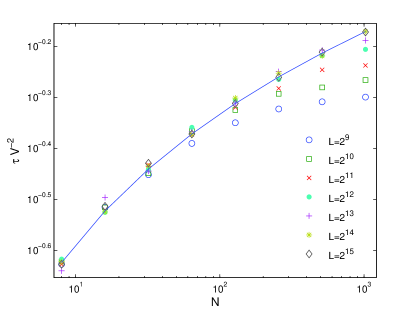
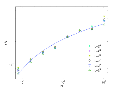
Figure 3: Rescaled Cover Time $\tau(N,V)$ versus the number of walkers making up the system and diffusing on a periodic chain (left panel) and cubic lattice (right panel). Different sizes are considered, as shown by the legend. Equation (6) provides the best fit when reactants concentration is small.

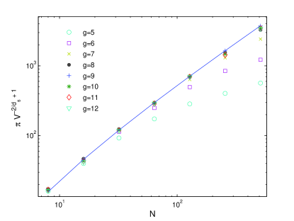
Figure 4: Rescaled Cover Jumps $\pi(N,V)$ for a system of walkers diffusing and reacting on a Sierpinski gasket (left panel) and on a cubic lattice with periodic boundary conditions (right panel). Different sizes are depicted, as shown by the legend. Equation (7) provides the best fit when the reactants concentration is small. Notice that in the latter case $\pi(N,V)$ is independent of $V$.

4 Numerical Results

We first consider final quantities, i.e. quantities measured when the excitation has covered the whole population of walkers. Subsequently, we will take into account the temporal evolution of the system by discussing quantities such as the average number of distinct walkers $\mathcal{S}(t)$ visited at least once by the excitation, as well as $\mathcal{S}(t,k)$ and $\mathcal{J}(t,k)$ representing the probability distribution of having $k$ distinct walkers visited at time $t$ and of having $h$ jumps performed at time $t$.

4.1 Cover Time and Cover Jumps

In this section we focus on numerical results concerning the Cover Time $\tau$ and the Cover Jumps $\pi$. We recall that $\tau$ has been defined as the average time it takes the excitation to reach all the $N$ walkers diffusing on the substrate considered. Analogously, $\pi$ represents the average number of jumps performed by the excitation within the time at which $\mathcal{S}=N$. Obviously, $\pi\leq\tau$.

In Figs. 3 and  4 a proper rescaling of data points confirms the analytical results discussed in the previous section (see equations (6) and (7)). In particular, in the low-density regime, $\tau(N,L)$ and $\pi(N,L)$ depend separately on $N$ and $L$ and their functional form is strongly affected by the topology of the lattice underlying the propagation (for example notice that for transient substrates $\pi$ gets independent of the size of the lattice).

4.2 Distinct walkers Visited

In Section 1 we introduced $\mathcal{S}(t)$ as the average number of distinct walkers which have been excited at least once at time $t$.

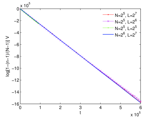
Figure 5: Rescaled number of distinct particles visited by the second-level random walker as a function of time for a periodic cubic substrate. Equation (9) holds for any (low) concentration chosen. The only free parameter in the fitting procedure is $\lambda_{d_{s}}^{fit}=2.65\pm 0.05.$

In Sec. 3 we analytically showed that, in the long-time regime, independently of the (finite) substrate topology $\mathcal{S}(t)$ grows exponentially with time (see equation (9)). On the other hand, in the early-time regime, for recurrent substrates, a functional dependence on the topology is expected, consistently with what found for a random walker on a finite lattice [12].

Let us first consider the case of a cubic structure for which the behavior of $\mathcal{S}(t)$ is not expected to display any crossover in time. Indeed, Fig. 5 confirms this: on the whole range of time, equation (9) is a good estimate for $\mathcal{S}(t)$ when the density is low. The slope of $V\log\left(1-\frac{\mathcal{S}(t)}{N}\right)$ also allows to derive an estimate for the constant $\lambda_{d_{s}}$. By fitting numerical data we find that $\lambda_{3}\simeq 2.65(5)$, $\lambda_{2}\simeq 6.84(4)$, $\lambda_{1}\simeq 10.01(8)$, (to be compared with those in Sec. 3.3, recalling that here $R=1$).

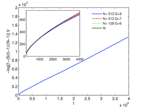
Figure 6: Time dependence for the number of distinct walkers excited at least once and diffusing on Sierpinski gaskets of different generations, as shown by the legend. The crossover between the two time regimes is apparent by comparing the plot in the large figure and the set of data depicted in the inset. The quantity $-\log(1-S(t)/N)V$ scales respectively as $t$ and $t^{{d_{s}}/{2}}$.

Now, let us consider low-dimensional substrates. The numerical simulations performed on the chain and on the Sierpinski gasket (see Fig. 6) support what previously stated. In particular, for the latter we show that, at long time, $\mathcal{S}(t)$ increases exponentially, analogously to what previously found for the cubic lattice. Conversely, at small times, deviations emerge: the pure-exponential growth is replaced by $e^{t^{{d_{s}}/2}}$ in agreement with equation (10).

In Sec. 1 we introduced the function $\mathcal{S}(k,t)$, representing the probability that, at time $t$, the number of walkers visited at least once by the excitation is $\mathcal{S}(t)=k$. In Sec. 3 we also derived a mean-field approximation for this quantity, valid in the low-density regime. We now discuss the pertaining results from numerical simulations.

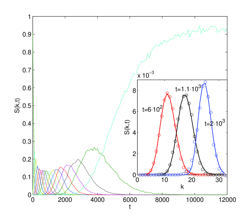
Figure 7: Main Figure: Probability distribution $\mathcal{S}(k,t)$ versus time $t$ for a system of $N~{}=~{}32$ walkers diffusing on a cubic lattice sized $L=16$ with periodic boundary conditions. Each curve represents a different (even) value of $k$: starting from the leftmost distribution $k=2,4,6,...,32$. Inset: Probability distribution $\mathcal{S}(k,t)$ versus number of visited random walkers $k$; three different instant of time are depicted in different colors: $t=6\cdot 10^{2},1.1\cdot 10^{3},2\cdot 10^{3}$. Data points ($\circ$) are fitted by a Poissonian distribution with average $\mu_{{d_{s}}}=\lambda_{{d_{s}}}\rho t$ in agreement with what stated in Sec. 3.4

.

In Fig. 7 the probability distribution $\mathcal{S}(k,t)$ is fitted by a Poissonian law with average $\mu$ linearly dependent on the density $\rho=\frac{N}{V}$ of the system. Moreover, the time $t_{peak}$ each distribution is peaked at depends on $k$ and it diverges logarithmically when $k\rightarrow N$ (see Fig. 8) according to equation (12).

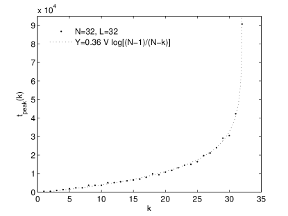
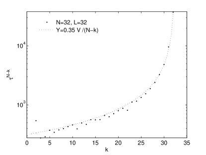
Figure 8: $t_{\mathrm{peak}}(k)$ and $\tau^{N-k}$ as a function of $k$ for a periodic cubic lattice. The dashed lines (whose equations are reported) represent the best fits in agreement with equations (12) and (13). The only free parameter is $\lambda_{d_{s}}$ and we get $\lambda_{d_{s}}^{fit}=2.79\pm 0.07$.

From the distribution $\mathcal{S}(k,t)$ it is also possible to measure the average lifetime $\langle t_{k}\rangle$ for the $k$-th state. This quantity diverges linearly as $k\rightarrow N$ as shown in Fig. 8 where results for the cubic lattice are depicted and fitted consistently with equation (13).

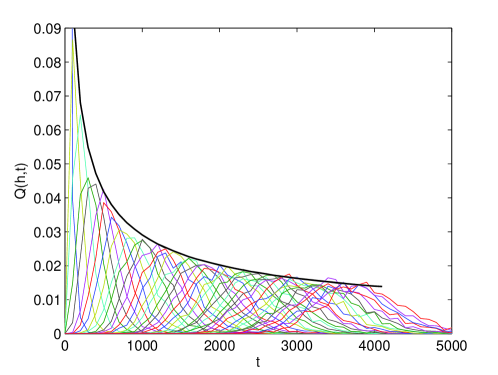
Figure 9: Probability distribution $\mathcal{J}(h,t)$ versus time $t$ for a system of $N=32$ walkers diffusing on a cubic lattice sized $L=16$, with periodic boundary conditions. Several curves are depicted, each referring to a different number of passages $h$ (selected one every 5 entries). As $h$ increases, the extremal point of the related distribution $t_{\mathrm{peak}}(h)$ gets larger, distributions are more and more overlapped and fluctuations get more important. The best fit for $\mathcal{J}(h,t_{\mathrm{peak}}(h))$ is represented by the black line $y~{}=~{}A~{}t^{B}$, with $A=1.11\pm 0.02,\,B=0.53\pm 0.01$. Data have been averaged over $1.8\cdot 10^{5}$ realizations.

An important feature emerging from Fig. 7 is the existence of a minimum for $\mathcal{S}(k,t_{peak})$. Indeed, there exists a value $\tilde{k}$ at which the distribution is maximally spread; in the average $\tilde{k}=\frac{N}{2}$ and, correspondently, the statistical knowledge we have about the system is minimum. From equation (9) we can estimate $\tilde{t}\approx\frac{V}{\lambda_{d_{s}}}\log 2$.

Finally, in Fig. 9 numerical results for $\mathcal{J}(h,t)$ are depicted. We recall that $\mathcal{J}(h,t)$ just represents the probability that the number of passages performed by the excitation is $h$ at time $t$. From the perspective of the energy-transfer mechanism this quantity is also of practical interest, especially in the case we allow for energy dissipation or emission during transfer. As shown in Fig. 9, there is no extremal point for the envelop of such distributions which is indeed characteristic of $\mathcal{S}(k,t)$.

5 Conclusions and perspectives

We have introduced and studied the diffusion of an excitation (or second-level random walker) on a population of $N$ random walkers diffusing on a given lattice (substrate) with finite volume $V$. This results in a stochastic process $\mathcal{X}(t)$ whose transition probabilities are themselves stochastic. The interest in this kind of problem is also motivated by the fact that it provides a model for systems of particles interacting by means of exchange energy transfer.

We showed that in the low-density regime ($\rho=\frac{N}{V}\ll 1$) $\mathcal{X}(t)$ can be mapped onto simpler processes, which allows the analytic calculation of the quantities characterizing the diffusion of the second-level RW. This analytic approach becomes rigorous only for homogeneous substrates, but yields reliable results also for fractal substrates. We presented numerical results supporting our analytical findings.

There are two main possible developments for this model. First, one can introduce a number $N_{e}>1$ of excitations jumping among the walkers. This would allow for the existence of several donors (excited walkers) in the system at the same time, and, possibly, of several excitations residing on the same walker. The rules governing the interaction between two donors (i.e., the existence of constraints on the number of excitations on a single walker) would have to be included in the model.

The second development consists in adding more levels of diffusion. If we define a set of $N_{e}>1$ excitations, we obtain a set of $N_{e}>1$ second-level stochastic processes. We can then define a collision rule for those stochastic processes (for example, two of them collide when the two excitations are on the same walker). Then, we can introduce a third-level stochastic process by allowing a third population of walkers diffuse on the second population (that of the excitations). The interplay between the properties of the second- and third-level stochastic processes (and a fourth-level one, and so on) could then be studied.

References

References

- [1] van Kampen NG 2001 Stochastic Processes in Physics and Chemistry, North-Holland Press
- [2] Förster T 1948 Ann. Phys. 2 55
- [3] Dexter D L 1953 J. Chem. Phys. 21 836
- [4] Havlin S and Ben-Avraham D 1987 Adv. Phys. 36 695
- [5] Burioni R and Cassi D 2005 J. Phys. A 38 R45
- [6] Yuste SB, Acedo L and Lindenberg K 2001 Phys. Rev. E 64 052102
- [7] Nemirovsky AM, M rtin HO, and Coutinho-Filho MD 1990 Phys. Rev. A 41 761
- [8] Weiss GH 1994 Aspects and Applications of the Random Walk, North-Holland Press
- [9] Montroll EW and Weiss GH 1965 J. Math. Phys. 6 167
- [10] Kozak JJ and Balakrishnan V 2002 Phys. Rev. E 64 021105
- [11] Agliari E submitted
- [12] Weiss GH, Havlin S and Bunde A 1985 J. Stat. Phys. 40 191