X-Ray Flaring on the dMe Star, Ross 154

Abstract

We present results from two Chandra imaging observations of Ross 154, a nearby flaring M dwarf star. During a 61-ks ACIS-S exposure, a very large flare occurred (the equivalent of a solar X3400 event, with $L_{X}=1.8\times 10^{30}$ ergs s^-1) in which the count rate increased by a factor of over 100. The early phase of the flare shows evidence for the Neupert effect, followed by a further rise and then a two-component exponential decay. A large flare was also observed at the end of a later 48-ks HRC-I observation. Emission from the non-flaring phases of both observations was analyzed for evidence of low level flaring. From these temporal studies we find that microflaring probably accounts for most of the ‘quiescent’ emission, and that, unlike for the Sun and the handful of other stars that have been studied, the distribution of flare intensities does not appear to follow a power-law with a single index. Analysis of the ACIS spectra, which was complicated by exclusion of the heavily piled-up source core, suggests that the quiescent Ne/O abundance ratio is enhanced by a factor of $\sim 2.5$ compared to the commonly adopted solar abundance ratio, and that the Ne/O ratio and overall coronal metallicity during the flare appear to be enhanced relative to quiescent abundances. Based on the temperatures and emission measures derived from the spectral fits, we estimate the length scales and plasma densities in the flaring volume and also track the evolution of the flare in color-intensity space. Lastly, we searched for a stellar-wind charge-exchange X-ray halo around the star but without success; because of the relationship between mass-loss rate and the halo surface brightness, not even an upper limit on the stellar mass-loss rate can be determined.

1. INTRODUCTION

Apart from the Sun, the best opportunities to study stellar magnetic phenomena at extremely low levels are provided by nearby stars. Of particular interest are the M dwarfs, whose lower photospheric temperatures and often higher coronal temperatures represent significantly different conditions from those of the solar atmosphere.

M dwarfs tend to be more active than F-G dwarfs, with approximately half of the former (the dMe stars) showing emission in H$\alpha$, the hallmark of flaring activity. Despite having surface areas only several percent as large as the Sun’s, dMe stars have X-ray emission that is usually comparable to or larger than the solar X-ray luminosity; the flaring coronae of M dwarfs would thus appear to present a much more dynamic environment than offered to us by the Sun. These conditions provide a means for determining how stellar activity differs from the solar analogy, with the ultimate goal of underpinning observational similarities and differences with the fundamental physics needed to describe the various activity phenomena on display.

Here we present analyses of two Chandra X-ray Observatory observations of the M3.5 dwarf Ross 154, which (counting Proxima Cen as part of the $\alpha$ Cen system (Wertheimer & Laughlin, 2006)) is the seventh nearest stellar system to the Sun. The original motivation for our primary observation, with the ACIS-S detector, was to constrain the stellar mass-loss rate by searching for X-ray emission from charge-exchange collisions of its ionized wind with the surrounding interstellar medium (ISM); Ross 154 is one of the few stars with a combination of distance and mass-loss rate that might be amenable to this technique using current observing capabilities (see §8). During the observation, the star underwent an enormous flare during which the X-ray photon count rate rose two orders of magnitude above the quiescent value. These X-ray data offer a rare glimpse of the time evolution of flaring plasma while simultaneous optical monitoring observations using the Chandra Aspect Camera Assembly provide insights into the response of the chromosphere and photosphere during the event. A second observation using the HRC-I detector provides only temporal information, but with superior statistical quality.

In §2 we summarize what is known about Ross 154. Sections 3 and 4 describe the X-ray and optical observations and data reduction. The analysis of the ACIS X-ray spectra is described in §5, and temporal analyses of the photon event lists and large flare light curve are presented in §6 and §7, respectively. Finally, we discuss our attempts to deduce the mass-loss rate of Ross 154 in §8 before summarizing our findings in §9.

2. THE TARGET

Ross 154 (Gleise 729, V 1216 Sgr) is a flaring M3.5 dwarf and lies at a distance of 2.97 pc (Perryman et al., 1997) towards the Galactic Center ($l=11.31^{\circ}$, $b=-10.28^{\circ}$; RA $=$ 18:49:49, Dec. $=-$23:50:10). Its X-ray luminosity, estimated at $6.0\times 10^{27}$ ergs s^-1 based on Röntgen Satellite (ROSAT ) measurements (Hünsch et al., 1999), is modest for active M dwarfs, which range up to nearly $10^{30}$ ergs s^-1 in quiescence. Its $\log(L_{X}/L_{\mathrm{bol}})$ value is -3.5 (Johns-Krull & Valenti, 1996), somewhat below the saturation limit of $\sim-3.0$ for active late-type stars (Agrawal, Rao, & Sreekantan, 1986; Fleming et al., 1993). RS CVn stars, which are close binary systems—often tidally locked—with high rotation rotation rates and flaring activity, have luminosities up to $\sim 10^{32}$ ergs s^-1 (Kellett & Tsikoudi, 1997).

Ross 154 is a moderately fast rotator, with $v\>\sin i=3.5\pm 0.5$ km s^-1 measured by Johns-Krull & Valenti (1996), indicating an age of less than 1 Gyr. Those authors also estimate a magnetic field strength of $2.6\pm 0.3$ kG with a filling factor $f=50\pm 13$%, somewhat weaker than the $\sim$4-kG fields with $f\gtrsim 50$% measured for three other more X-ray-luminous and faster-rotating dMe stars: AD Leo (Saar & Linsky 1985), EV Lac (Johns-Krull & Valenti 1996), and AU Mic (Saar 1994; all three stars). Its photospheric metallicity is roughly half-solar based on the estimated iron abundance of [Fe/H]$\sim-0.25$ reported by Eggen (1996), and the presence of optical emission lines from Fe I, Si I, and Ca I indicates a surprisingly cool chromosphere (Wallerstein & Tyagi, 2004).

Ross 154 has been detected by a number of high-energy observatories— Einstein (Agrawal et al. 1986; Schmitt et al. 1990), ROSAT  (Wood et al. 1994; Hünsch et al. 1999), and the Extreme Ultraviolet Explorer (EUVE; Bowyer et al. 1996; Lampton et al. 1997; Christian et al. 1999) —but was never studied in any detail, and no significant flares were seen in the relatively short exposures obtained by those missions.

3. THE OBSERVATIONS

Two sets of Chandra data were analyzed. The first observation was conducted for 60625 s beginning on 2002 September 9 at 00:01:20 UT (Chandra time 147916880). The primary objective was to look for a faint stellar-wind halo around the star so no grating was used, despite the brightness of the coronal emission and the expectation of severe pileup in the source core. This measurement (ObsId 2561 (catalog ADS/Sa.CXO#obs/02561)) used the ACIS-S3 backside-illuminated CCD chip in Very Faint (VF) mode with a subarray of 206 rows that allowed a short 0.6-s frame time to be used, thus reducing the degree of event pileup.

Standard Chandra X-ray Center pipeline products were reprocessed to level 2 using the Chandra Interactive Analysis of Observations (CIAO) software version 3.4 with calibration data from CALDB 3.3.0.1, which applies corrections for charge-transfer inefficiency in all ACIS CCDs and for contamination build-up on the ACIS array. Eight weak secondary sources were then removed from the source field (Fig. 1a) and VF-mode filtering was applied to reduce the background, except near the core of the primary source as explained in §4. No background flares were observed in the data.

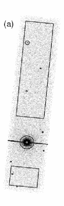
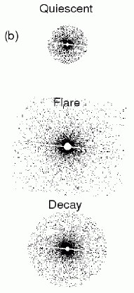
Figure 1.— ACIS data extraction regions. Panel (a) shows the annulus used for Quiescent spectra data around the primary source, small circles around weak secondary sources, and two rectangular background regions; also note the bright readout streak running approximately horizontally through the primary source. Panel (b) shows the spectral extraction regions for the Quiescent, Flare, and Decay phases; the spatial scale is twice that of panel (a). Spectral extractions exclude the piled-up core and the readout streak, the latter of which may have a slightly different detector gain from non-streak regions. Streak data, however, are included in temporal analyses.

Examination of the X-ray light curve (Fig. 2) after excluding the piled-up core of the target reveals three temporal phases in our observation: a quiescent phase; a very large flare; and the flare decay. We also obtained a simultaneous optical light curve using data from the Chandra aspect camera.

Figure 2.— Optical and X-ray light curves from the ACIS observation, with time bins of 20.5 and 100 s, respectively (500 s in X-ray detail). Zero time corresponds to the beginning of the observation at 2002 September 9 at 00:01:20 UT. X-ray light curve is for $E=250-6000$ eV with a spatial filter comprising an annulus of radii 6 and 60 pixels (to exclude the piled-up core) plus a 6-pixel-wide box along the readout streak. The annulus used for the Quiescent Detail light curve had radii of 4 and 40 pixels. In the absence of pileup, so that core events could also be used, the counting rate would be $\sim$25 times higher. Note the small optical flare at the very beginning of the X-ray flare.

The second observation (ObsId 8356 (catalog ADS/Sa.CXO#obs/08356)) occurred on 2007 May 28 beginning at 4:19:18 UT (Chandra time 296713158) and ran for 48511 s, excluding two 32.8-s periods that did not meet Good Time Interval criteria. This HRC-I calibration measurement was made in parallel with a measurement of the ACIS background, in which ACIS is placed in a “stowed” position where it is both shielded from the sky and removed from the radioactive calibration source in its normal off-duty position. With ACIS in the stowed position, the HRC-I is 75 mm away from its nominal on-axis position but can be used for off-axis observations to calibrate the Chandra point spread function (PSF) and measure small-scale gain uniformity. When ACIS is collecting data in its standard telemetry mode the HRC can operate simultaneously, albeit with severe telemetry restrictions, in its Next-In-Line (NIL) mode with a limit of $\sim$3.5 counts s^-1. Ross 154 is one of a handful of isolated sources with a counting rate and other parameters suitable for such NIL-mode calibration observations.

The HRC-I observation was made $25.62^{\prime}$ off axis (Y offset = $-11.83^{\prime}$, Z offset = $22.73^{\prime}$) using a 10-tap$\times$10-tap ($5.61^{\prime}\times 5.61^{\prime}$ ) window of the detector, large enough to encompass the out-of-focus source image and also provide a suitably large region to determine the background level (see Fig. 3). Within the windowed detector region the background accounted for $\sim$2.6 counts s^-1 and the total rate during source quiescence was $\sim$3.0 counts s^-1. At least one large flare exceeded the telemetry limit. The HRC-I has essentially no spectral information and so these data were used only for the microflaring study presented in §6. Until then our discussion will refer exclusively to the ACIS observation.

Figure 3.— Image of the HRC-I off-axis observation. The inner ellipse marks the source region used for microflaring analysis. The background region used to construct the light curve in Fig. 8 lies outside the larger ellipse.

4. ACIS DATA EXTRACTION

4.1. Optical Monitor Data

Although the capability is rarely used, one or more of the eight Chandra Aspect Camera Assembly (ACA) “image slots” can be assigned to monitor selected sky locations, with a practical faint limit of roughly $V=12$. For comparison, the guide stars used for aspect determination and to correct for spacecraft dither generally have magnitudes between $V=6$ and 10, and Ross 154 has a magnitude of $V=10.95$. The faint limit is largely determined by pixel-to-pixel changes in the optical CCD dark current, with temporal variations on scales of typically a few ks. The effects of these background variations are significant in our observation, but were largely removed by averaging data collected when the source centroid dithered more than $\sim$3.5 pixels away from the pixel under consideration and then subtracting the average bias within each pixel. Quantum efficiency nonuniformity was mapped by analyzing data from times when the source centroid was within 0.1 pixels of the center of the peak pixel; the flat field corrections thus derived were never more than 3%.

In addition to having a low signal level, the optical monitoring of Ross 154 suffered a loss of tracking halfway through the quiescent phase of the observation, causing the star to wander within its 8$\times$8-pixel ACA window (with integration time of 4.1 s per frame) as the spacecraft dithered with a period of 707.1 s in pitch and 1000.0 s in yaw, causing semi-periodic dips of up to 14% in the light curve as some of the source flux was lost near the edges of the window. Various flux correction schemes were tried, but the best results were obtained by summing the background-subtracted counts within a $5\times 5$ box centered on the highest-count pixel and discarding all data from cases where the $5\times 5$ box did not fit within the $8\times 8$ ACA window. The resulting optical light curve is shown in the top panel of Figure 2, revealing a 0.15-magnitude flare and a smaller precursor; these are discussed in more detail in the context of the X-ray flare behavior in §7.

4.2. X-Ray Data

After removing secondary sources from the X-ray data, a background region was obtained by excluding the dithered edges of the field and a 300-pixel-wide ($147^{\prime\prime}$) region around the source (Fig. 1a). Even with the large exclusion region around the main source, the flare was so intense that excess counts could still be seen in the background light curve so we excluded 2000 s around the flare peak. The remaining background data show no evidence for temporal variability.

Table 1ACIS Spectral Data Extraction Parameters

I
		Gross	Excluded	Outer	Streak
	Time	Exposure	Core Radius	Boundary	Width
Phase	(2002 Sep 9 UT)	(s)	(pixels)	(pixels)	(pixels)
I
Quiescent	00:01:20 – 11:51:40	42620	4	40 (radius)	4
Flare	11:51:40 – 12:38:20	2800	8	202 (box height)	6
Decay	12:38:20 – 16:51:45	15205	5	80 (radius)	5

Ross 154 is such a bright X-ray source that even during quiescence it produced a strong CCD readout streak and the core was very heavily piled-up. To obtain undistorted spectra we excluded the core, with a different radius for the quiescent, flare, and decay phases of our observation (see Table 1), based on studies of spectral hardness ratios and VF-filtering losses as a function of radius. The hardness ratio method is based on the fact that piled-up spectra shift lower energy flux to higher energies; hardness ratios of spectra from events near the core can therefore be compared with hardness ratios at larger radii where pileup is known not to occur. This effect is masked to some extent by the energy dependence of the Chandra PSF, which becomes broader as energy increases, so a more effective means of detecting pileup is to study the distribution of events that are removed by VF filtering.

In ACIS Faint (F) mode data, the distribution of charge within a $3\times 3$-pixel ‘island’ is measured to determine if a valid X-ray event has been detected. VF filtering uses $5\times 5$-pixel islands and discards events that have significant charge in the outer pixels. It is therefore much more sensitive to event pileup than F mode, and if an event is not removed by VF filtering it is almost guaranteed to be a single unpiled event. We studied the distribution of events discarded by VF filtering as a function of radius for each observation phase and chose the excluded-core radii listed in Table 1 such that no more than 1.3% of the total flare-phase events outside that radius (0.7% for the quiescent phase and 0.8% for the decay) would be excluded by VF filtering. The net pileup fraction of the extracted events is estimated to be less than 0.5%. Close to the core but still within the extraction region, nearly all the ‘bad VF’ events are in fact valid and unpiled. To keep those events, and since the number of background events is negligible within such a small region, VF filtering was not applied out to a radius of twice the excluded core radius.

The outer boundaries of the spectral extraction regions for each phase were chosen to keep the fraction of background events small ($<4$% for the Quiescent phase and less for the others) while including as many X-ray source events as possible. The readout streaks, which do not suffer from pileup because of their very short effective exposure times, were included in temporal analyses but excluded from spectral analyses (see Fig. 1 and Table 1) because of concerns that the effective detector gain might be sufficiently different from that of non-streak events to distort the spectra. A gain increase of $\sim$7% has been reported by Heinke et al. (2003) in streak spectra from the front-illuminated ACIS-I3 chip at the Ir-M absorption edge (a spectral feature near 2 keV arising from the Chandra mirrors), and an increase of $\sim$2.5% was measured in the back-illuminated ACIS-S3 chip. It is not yet clear if this effect is energy dependent (private communication, R. J. Edgar), and our streak spectra had too few counts to measure a gain shift, other than to say that it must be no more than a few percent at the Ir-M edge and no more than 10% at energies down to $\sim$500 eV.

Response matrices (RMFs) and effective area files (ARFs) were created for each extraction region according to the psextract script, which uses the mkacisrmf tool. ARF correction functions were then created to account for exclusion of the source core as described below.

4.2.1 Effective Area Corrections

Although exclusion of the source core eliminates the spectrum-distorting effects of pileup, which are so severe in this case that they cannot be modeled, it introduces other modifications to the source spectrum because of the energy dependence of the telescope point spread function (PSF); low energy X-rays are more tightly focused than those with high energy.

We modeled the PSF using the Chandra Ray Tracer (ChaRT; Carter et al. 2003) tool using 22 million rays and then projected them onto the ACIS detector using the MARX simulator, producing 7.5 million detected events ranging from 0.1 to 8 keV with half of them below 3 keV. The MARX parameter DitherBlur was changed from the default value of 0.35^′′ to 0.28^′′ to properly model the effects of turning pixel randomization off during reprocessing of the observation with acis_process_events. The data extraction regions listed in Table 1 were then applied to the simulated data, and extracted spectra were compared to the full-detector spectrum in order to derive effective area correction functions for each phase (see Fig. 4a). Near the peak of the detected source spectra around 1 keV, only 2 or 3% of the potential event detections are extracted. The average Quiescent count rate after correcting for the extraction efficiency is 2.0 cts s^-1.

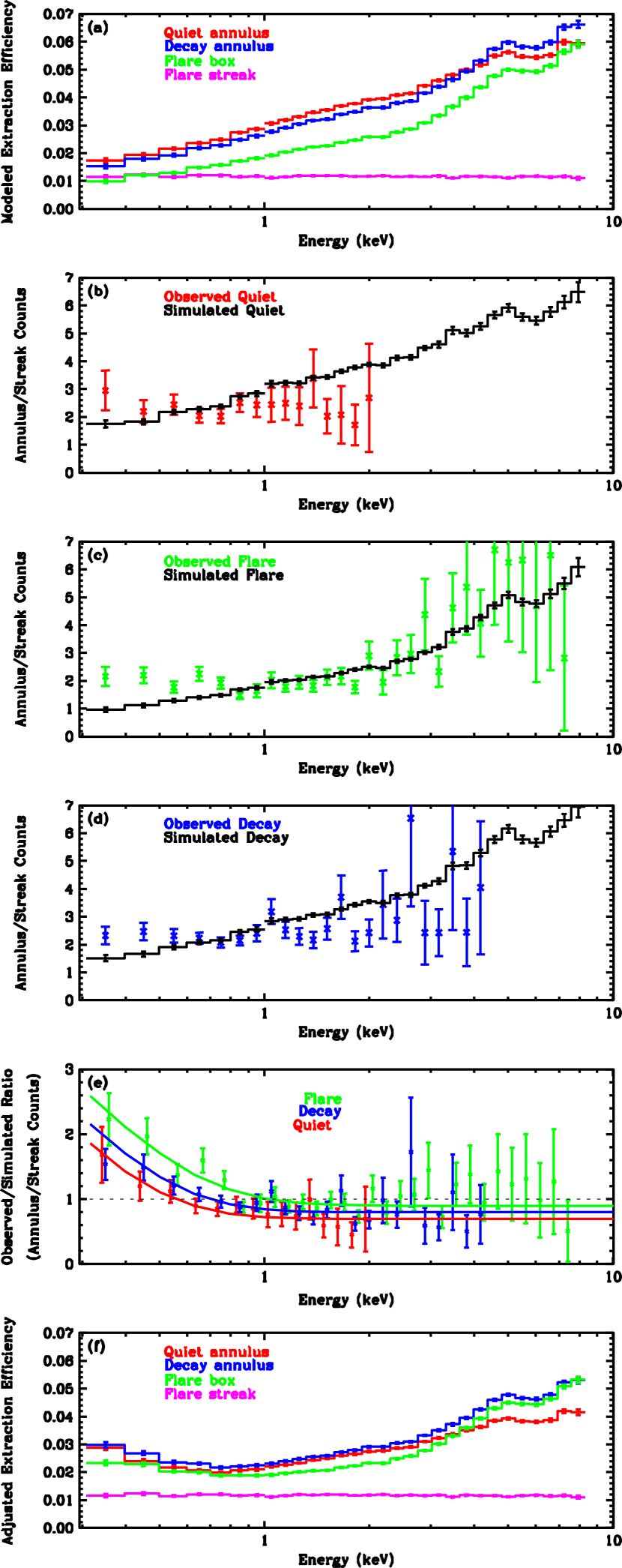
Figure 4.— Simulated and observed results on data extraction efficiency. Bins are 100 eV below 1 keV, and logarithmic (25 per decade) above 1 keV. ($a$): Only a small fraction of the total source flux is extracted using annular regions that exclude the source core, particularly at low energies where focusing is best. Extractions along the readout streak (excluding the core) have much less energy dependence. ($b$,$c$,$d$): Ratio of counts in annular and streak extraction regions for Quiet, Flare, and Decay phases, for simulated and observed data. ($e$): Ratio of observed and simulated results from ($b$,$c$,$d$) for each phase. The observed ratio is larger than the simulated ratio at low energies, suggesting the simulated annular extraction efficiencies are too low. ($f$): Adjusted annular extraction efficiencies, after applying the smooth correction functions in ($e$) to results in ($a$).

Fig. 4a also shows the extraction efficiency for the readout streak during the Flare phase, using a 6-pixel-wide box and excluding a 20-pixel-radius around the source core. Readout-streak efficiencies are very similar for all three phases and nearly flat as a function of energy since the streak primarily comprises events from the core of the source, where energy dependent PSF effects are relatively minor. Some adjustments to the model streak results were required because MARX simulates full-chip (1024-row, 3.2-s frametime) ACIS operation while the observation used 206 rows with a 0.6-s frametime. The effective exposure time for the full-length streak is 7% larger in the observation than in the simulation but less of the streak is extracted (162 of 206 rows versus 988 of 1024, a relative difference of 23%), yielding a net adjustment of $\sim$14% to the extraction efficiency (observed lower than simulated).

ChaRT simulations of the PSF are known to have small errors, and when excluding the core such errors may be relatively large compared to the remaining fraction of source flux. We therefore compared the simulation’s predictions of the ratio of annular and streak events versus the observed ratio for each observation phase. As seen in Fig. 4b, c, and d, uncertainties are dominated by observational statistics and are especially large at high energies where there are few counts, but the simulations match observation reasonably well except at low energies. These discrepancies are presumably due to underprediction of the enclosed count fraction in the outer core of the PSF at low energies where focusing is best. As noted in §4.2 there may be small gain shifts in the streak spectra, but the effects on apparent streak extraction efficiency would be much smaller than the discrepancies seen. Further evidence that the simulation’s effective area corrections are suspect below $\sim$600 eV is provided by varying the energy range of spectral fits, as explained in §5.

Based on the data points in Fig. 4b–d, Fig. 4e plots the ratio of simulated and observational results, along with smooth curves that approximately follow the results for each phase. Each curve shows how the ratio of simulated extraction efficiencies for annular and streak data regions would have to be adjusted to bring it into accord with the observed ratio. If one assumes that the simulated streak extraction efficiency is correct, as one would expect since the PSF (or rather, line spread function) of the readout streak has so little energy dependence, then the smooth curve can be used as a correction factor for the annular-region extraction efficiency derived from the ChaRT/MARX simulation. Fig. 4f shows the simulation extraction efficiencies from Fig. 4a multiplied by those empirical correction factors, yielding what we will refer to as “adjusted extraction efficiencies”. Uncertainties in the adjusted efficiencies are relatively large at higher energies, but this is because of the small number of counts and the effect on spectral fits is modest.

5. SPECTRAL ANALYSIS

Spectral analysis was performed with the CIAO Sherpa fitting engine (Freeman et al., 2001). First, the adjusted extraction efficiency curves (Fig. 4f) were fitted with smooth functions (the sum of five Gaussians) to be used in conjunction with the ARFs (as multiplicative factors) during spectral fitting. The coronal emission itself was modeled using xsvapec models based on the plasma emission code APEC (Smith et al., 2001a). Parameter estimation was performed using the modified $\chi^{2}$ statistic (Gehrels, 1986), with some rebinning at higher energies to ensure at least 20 counts per bin.

Fits extended down to 350 eV, below which the ACIS-S response becomes increasingly uncertain, with upper energy limits for each phase determined by the level of source emission versus background (see Table 2). Different energy ranges were also tried, with variable effects on the fitting results. Fits of the Quiescent spectrum down to 200 eV led to overpredictions of $\sim$20% in the flux below 500 eV, while fits using a lower limit of 500 eV yielded poor constraints on the O abundance. Fits to the Flare and Decay spectra were less sensitive to the lower limit, and in all cases varying the upper limit of the fit range had relatively little effect.

Table 2Spectral Fitting Results

I
	Quiescent			Flare			Decay
Parameter	1-$T$	2-$T$		1-$T$	2-$T$		2-$T$
I
Fit range (keV)	0.35–3.0			0.35–8.0			0.35–8.0
Counts in fit	1802			4829			4891
Est. background	74			65			172
Deg. of freedom	63	61		164	162		125
Reduced $\chi^{2}$	0.61	0.53		0.99	0.78		0.71
$kT_{1}$ (keV)	$0.46_{-0.05}^{+0.03}$	$0.98_{-0.41}^{+0.21}$		$2.95_{-0.20}^{+0.27}$	$3.71_{-0.26}^{+4.30}$		$1.91_{-0.12}^{+0.12}$
$kT_{2}$ (keV)	$\cdots$	$0.29_{-0.04}^{+0.05}$		$\cdots$	$0.41_{-0.07}^{+1.17}$		$0.37_{-0.05}^{+0.04}$
EM1 ($10^{50}$ cm-3)	$19.8_{-2.4}^{+2.5}$	$4.1_{-1.4}^{+5.8}$		$341_{-26}^{+36}$	$271_{-20}^{+20}$		$12.7_{-2.4}^{+2.8}$
EM2 ($10^{50}$ cm-3)	$\cdots$	$10.8_{-7.6}^{+3.4}$		$\cdots$	$26_{-6}^{+306}$		$27.3_{-3.0}^{+3.0}$
Lum. ($10^{27}$ erg s-1)	9.35	8.66		449	464		51.1
OCNS abundance	$0.12_{-0.04}^{+0.05}$	$0.13_{-0.05}^{+0.07}$		$0.21_{-0.21}^{+0.47}$	$0.38_{-0.20}^{+0.26}$		$0.42_{-0.13}^{+0.17}$
NeAr abundance	$0.29_{-0.05}^{+0.07}$	$0.34_{-0.21}^{+0.24}$		$1.39_{-0.89}^{+0.90}$	$2.15_{-0.59}^{+0.71}$		$1.65_{-0.36}^{+0.48}$
MgNaAlSi abund.	$0.10_{-0.06}^{+0.06}$	$0.15_{-0.13}^{+0.20}$		$0.00_{-0.00}^{+0.10}$	$0.44_{-0.44}^{+0.54}$		$0.56_{-0.25}^{+0.32}$
FeCaNi abund.	$0.04_{-0.01}^{+0.01}$	$0.19_{-0.11}^{+0.10}$		$0.27_{-0.13}^{+0.14}$	$0.41_{-0.38}^{+0.18}$		$0.40_{-0.10}^{+0.13}$

Note. — Quoted uncertainties are formal 68% confidence intervals for the fits and do not include systematic uncertainties, such as those for the effective area of a data extraction region.

Because of the modest resolution and statistical quality of our spectra, we grouped elements with similar first ionization potential (FIP; in parentheses) as follows (see §5.4 for the reasoning behind FIP grouping): C, N, O, and S (11.3, 14.5, 13.6, and 10.4 eV); Na, Mg, Al, and Si (5.1, 7.6, 6.0, 8.2 eV); Ca, Fe, and Ni (6.1, 7.4, 7.6 eV); Ne and Ar (21.6, 15.8 eV). Element abundances were determined relative to the solar photospheric abundances of Anders & Grevesse (1989), which is the Sherpa default. More recent photospheric abundance tabulations are available (e.g., Grevesse & Sauval, 1998; Asplund, Grevesse, & Sauval, 2005), but the effect on our fit results (in terms of abundances relative to H) of using different assumptions is negligible, as confirmed by trials using the Asplund et al. (2005) abundances, and as expected since each element grouping typically has one dominant species. O emission dominates that from N and C because the ACIS effective area decreases rapidly toward lower energies, and there is virtually no S emission in the quiescent spectrum. Ne emission similarly dominates that from Ar. Abundances for Mg and Si, which have very similar FIP, are roughly an order of magnitude larger than those for Na and Al, and Fe likewise dominates Ca and Ni. Abundance linkages were studied in more detail for the flare spectrum, as described in §5.2.

Our analysis assumes that quiescent-phase emission is always present at a constant level, with added components for the flare and decay phases representing localized emission. Quiescent fit parameters are therefore frozen during flare and decay fitting, with the normalization adjusted for the differing exposure time and extraction region efficiency of each phase. The quiescent emission is completely overshadowed by higher-temperature components during the flare and decay, however, so its inclusion has little effect on those fits. The background is scaled and subtracted and contributes $\sim$4% of the counts in the fits’ energy ranges (less for the flare). Abundances are free to vary for each phase, subject to the FIP grouping described above. Interstellar absorption to this nearby source is completely negligible at the energies of relevance here ($N_{H}\lesssim 1\times 10^{18}$ cm²; Wood et al. 2005). Fit results are summarized in Table 2 and described in detail below, and the spectra are shown in Figure 5.

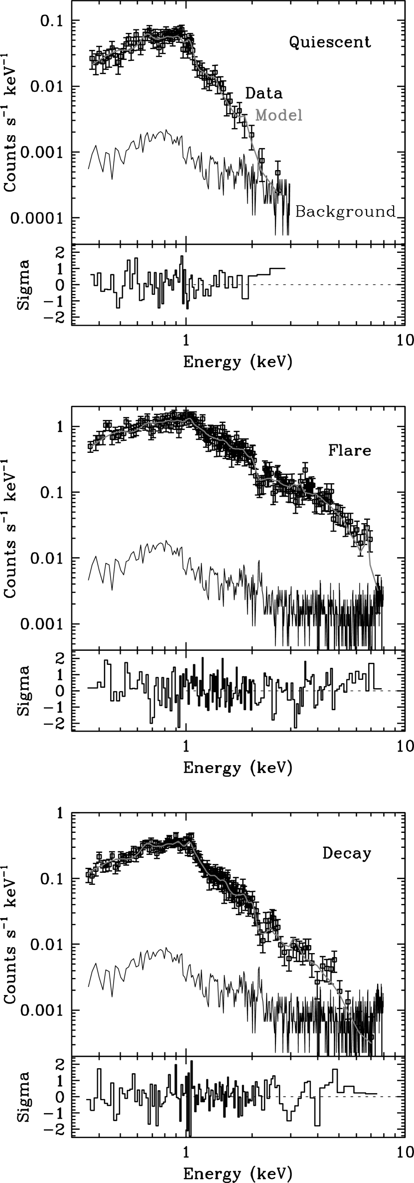
Figure 5.— Fits to spectral data, using the Quiescent “1-$T$,” Flare “2-$T$,” and Decay models listed in Table 2. Data are background-subtracted.

5.1. Quiescent Spectrum

As can be seen in Table 2, results for one- and two-temperature fits to the quiescent spectrum are quite similar, apart from a marginally significant difference in Fe abundances. Using two temperatures reduces the $\chi^{2}$ slightly, but the $F$-test significance of the second component is 0.29, much larger than the typical threshold of 0.05 for using a more complex model. We therefore refer to the 1-$T$ fit in all subsequent discussions unless otherwise noted. The fact that the reduced $\chi^{2}$ is significantly less than 1 (0.61) is likely a reflection of the modest number of counts. The similarity of abundances from the 1-$T$ and 2-$T$ fits, however, suggests that the derived values are realistic.

The total X-ray luminosity is $\sim 9\times 10^{27}$ erg s^-1, somewhat higher than the value of $6\times 10^{27}$ erg s^-1 estimated from ROSAT  observations (Hünsch et al., 1999). The difference is probably due to a combination of real source variability and uncertainties in spectral modeling; uncertainties in spectral extraction efficiencies (Fig. 4e) are largest the low energies, leading to relatively larger uncertainties in luminosity during quiescence than in the flare and decay phases.

The best-fit temperature is $T=5.0\times 10^{6}$ K ($kT=0.43$ keV) and the 68% confidence intervals for the abundances are $0.29^{+0.07}_{-0.05}$ for Ne (and Ar), $0.12^{+0.05}_{-0.04}$ for O (and C, N, S), $0.10^{+0.06}_{-0.06}$ for Mg (and Na, Al, Si), and $0.04^{+0.01}_{-0.01}$ for Fe (and Ca, Ni; the 2-$T$ fit had higher Fe abundance but with large uncertainties). Abundance-FIP correlations are discussed in detail in §5.4 but we note that in quiescence, the derived element abundances correlate (with modest significance) with FIP.

To study relative abundances in more detail and aid comparisons of quiescent and flare abundances, we studied $\chi^{2}$ as a function of the Ne/O abundance ratio by freezing Ne/O and refitting the data (see Figure 6). The result is a best-fit ratio of 2.4 with a $2\sigma$ confidence range (95.5%, $\Delta\chi^{2}=4.0$) for between 1.3 and 4.1, somewhat less than the value found from the flare spectrum (see §5.2). A study of the Fe/O ratio shows a similar enhancement during the flare, but the significance of this result vanishes if the quiescent Fe abundance from the 2-$T$ fit is used instead of that from the 1-$T$ fit. Uncertainties on the flare Mg abundance are too large to draw any conclusions regarding a difference from the quiescent abundance.

5.2. Flare Spectrum

One- and two-temperature models were also employed to fit the flare spectrum with, as noted above, an underlying fixed quiescent component. While the 1-$T$ fit gives a formally adequate fit with reduced $\chi^{2}=0.99$, the 2-$T$ model provides a visibly much better fit at low and high energies. We therefore used the 2-$T$ model, although both fits yield consistent results with respect to element abundances. Note that the upper limits on the two components’ temperatures are not well constrained, leading to a large uncertainty on the cooler component’s emission measure.

The power of this flare is remarkable. At its peak (approximately 3.8 times the average power during the flare phase we defined), the energy flux that would be observed 1 AU from the star reached 0.34 W m^-2 in the GOES solar flare energy band (1–8 Å, or 1.55–12.4 keV), corresponding to an X3400 solar flare. Over the full X-ray band (0.25–11 keV), the peak luminosity is $\sim 1.8\times 10^{30}$ erg s^-1 (13% of the $L_{bol}$ listed by Fleming, Schmitt, & Giampapa 1995), and the total radiated energy including the extrapolated decay phase is $\sim 2.3\times 10^{33}$ erg. The only flares from isolated M stars significantly more energetic than this were observed on EV Lac by the Advanced Satellite for Cosmology (ASCA; Favata et al., 2000) and EQ1839.6+8002 by Ginga (Pan et al., 1997). Both those events were roughly ten times more powerful than the Ross 154 flare.

In addition to its power and high temperature—note the Fe XXV emission feature at 6.7 keV in Figure 5—an interesting aspect of the flare is the large enhancement of Ne relative to its quiescent value. While all the abundances rise during the flare (uncertainties for Mg are too large to draw any conclusions), the increase for Ne is the most significant. Because abundance ratios are often more reliable than absolute values, we again applied the analysis procedure described in §5.1 to study the significance of the Ne/O ratio (see Figure 6). We conclude that there is roughly a 90% statistical likelihood that Ne is relatively more abundant during the flare than during quiescence, with a best-fit Ne/O ratio of 5.7, compared to the quiescent ratio of 2.4. The 90% statistical likelihood, however, does not take into account systematic uncertainties from our extraction efficiency modeling.

Figure 6.— Confidence intervals for the Ne/O abundance ratio (normalized to solar photospheric abundances) in fits to quiescent (solid curves) and flare (dashes) spectra. The 1-$T$ model was used for the quiescent fits and the 2-$T$ model for the flare (see Table 2).

The flare was hot enough to generate substantial emission from H-like and He-like Ar, unlike during the quiescent phase, so we unlinked the Ar and Ne abundances in an alternative fit. The best-fit results yielded very large uncertainties for Ar with negligible effect on the Ne abundance or any other parameters. Fits that unlinked S (from O, C, and N) and Si (from Mg, Na, and Al) provided similarly uninformative results.

As noted above, the interstellar column density to Ross 154 is so low ($N_{H}<10^{18}$ cm^-2) that X-ray absorption is negligible. There has been one report, however, of a large increase in absorbing column density (to $\sim 2.7\times 10^{21}$ cm^-2) during a large flare observed on Algol (B8 V + K2 IV) by BeppoSAX, presumably the result of a coronal mass ejection from the K2 secondary in association with the flare onset (Favata & Schmitt, 1999). We therefore added an absorption term to our flare model, but the fit drives $N_{H}$ to zero. Freezing $N_{H}$ has no significant effect on the fit for values up to a few times $10^{20}$ cm^-2, but fits with $N_{H}$ much beyond $10^{21}$ cm^-2 are noticeably poor.

5.3. Decay Spectrum

One-temperature models give unacceptable fits to the decay spectrum and Table 2 therefore lists results only from 2-$T$ models. Physically, one would expect temperatures and abundances to be intermediate between the quiescent and flare values, and probably closer to the latter since we observe the portion of the long-lived decay immediately following the flare. The fit therefore gives sensible results, but the model and fit uncertainties are too large to draw any firm conclusions regarding element depletions or enhancements.

Before discussing implications of the fit results, it is worth recalling that the real uncertainty in any physical parameter is always larger than the formal fitting error. Although the fit results in Table 2 are fairly insensitive to the choice of model, model assumptions inevitably affect the values of derived parameters, as do many other factors such as atomic data uncertainties, limited energy resolution, and calibration errors. The latter can be especially important with regard to the interdependence of derived emission measures and element abundances, as illustrated by Robrade & Schmitt (2005) in fits to XMM-Newton data from several instruments; much of the (modest) disagreement between results from fits to the MOS and other instruments can likely be attributed to recently discovered spatially dependent response function variations in the MOS detectors caused by cumulative radiation exposure (Stuhlinger et al., 2006; Read et al., 2006). Although calibration errors in ACIS should not be a significant issue here, exclusion of the piled-up source core and attendant energy-dependent modifications to the effective area have introduced difficult-to-estimate uncertainties into our fits. Uncertainties in atomic data used in the fits are relatively small and, as described above, we have taken some care to study the sensitivity of our model assumptions and parameters, but the uncertainties on the fit values listed in Table 2 should be viewed as lower limits.

5.4. Abundances Discussion

Coronal abundance patterns seen in stars with solar-like to very high activity levels currently appear to deviate from expected photospheric values according to element first ionization potentials. In the solar case, low-FIP elements ($\lesssim 10$ eV, e.g., Si, Fe, and Mg) appear enhanced by typical factors of 2-4 compared with high-FIP elements ($\gtrsim 10$ eV, e.g, O, Ne, Ar) which have roughly photospheric values (e.g., Feldman, 1992, and references therein). In stars, there appears to be a steady transition from a solar-like FIP effect to “inverse-FIP effect” as activity level rises (e.g., Drake et al., 1995; White et al., 1994; Telleschi et al., 2005; Audard et al., 2003; Güdel et al., 2002b).

Several abundance studies of active M dwarfs suggest they share a pattern similar to that of higher mass active stars. Robrade & Schmitt (2005, see also ) analyzed XMM-Newton observations of four M dwarfs with spectral types similar to that of Ross 154, namely EQ Peg (GJ 896AB; a wide binary with M3.5Ve and M4.5Ve components), AT Mic (GJ 799AB; a tidally-interacting M4.5Ve+M4V binary), EV Lac (GJ 873; M3.5Ve), and AD Leo (GJ 388; M3.5e). They conclude that all these stars exhibit a similar abundance pattern: a remarkably flat abundance-versus-FIP relationship (roughly half-solar photospheric) from Si (8.15 eV) to N (14.53 eV), with only Ne (21.56 eV) showing a conspicuous enhancement. This pattern is also reminiscent of that found for Proxima Cen (GJ 551) by Güdel et al. (2004) and for the dMe active spectroscopic binary YY Gem (Castor C) by Güdel et al. (2001) from XMM-Newton observations.

Adopting the 2-$T$ abundance results in Table 2, we find Ross 154 is broadly consistent in relative abundances with those from the earlier studies of M dwarfs. We find no significant deviation from a solar mixture in terms of the relative abundances of the OCNS, MgNaAlSi, and FeCaNi groups, but a significantly larger relative abundance of the NeAr group in quiescent, flare and decay spectra. There is some indication that the coronal metallicity (i.e. all metals scaled together) differs between quiescent and flare/decay phases: both FeCaNi and OCNS groups appear more consistent with a value of 0.4 times that of Anders & Grevesse (1989) during the decay, compared with $\sim 0.15$ during quiescence. This is confirmed by 2-$T$ model fits in which all elements were tied to their relative solar values (except for the Ne/O ratio which was fixed at 2.4) and only the overall metallicity was allowed to vary. The metallicity rises from the quiescent value of $\sim 0.15$ to $\sim 0.55$ in the flare, with a best-fit value of $\sim 0.45$ during the decay (but statistically consistent with the flare value). The flare and decay metal abundances are essentially the same as the photospheric estimate of Eggen (1996).

The Ross 154 abundance pattern and Ne/O abundance ratio is similar to those of the Robrade & Schmitt (2005) sample, although during the flare there is a suggestion at the $1.5\sigma$–$2\sigma$ level of a Ne/O increase (see §5.2 and Table 2). The Ne/O ratio is interesting in the context of understanding solar structure and its distribution in the coronae stars of different activity level (e.g., Basu & Antia, 2004; Bahcall et al., 2005; Drake & Testa, 2005). Drake & Testa (2005) found a remarkably constant Ne/O abundance ratio that is $\sim$2.4 times higher than the currently favored solar ratio of 0.15 by number (e.g., Anders & Grevesse, 1989; Asplund, Grevesse, & Sauval, 2005; Young, 2005; Schmelz et al., 2005; Landi, Feldman, & Doschek, 2007) in a sample of mostly active stars over a wide range of spectral type (and as seen in Ross 154). They argue that a FIP-based fractionation mechanism is unlikely to result in such consistent Ne/O ratios when the Fe/O ratio in the same stars varies over an order of magnitude (see, e.g., Güdel, 2004), and suggest instead that the higher ratio—including that found for the M dwarfs analyzed by Robrade & Schmitt (2005)—represents underlying photospheric values. In this scenario, the M dwarfs appear to exhibit coronal abundances that reflect their relative photospheric values but that differ in terms of a global metal depletion factor.

The quiescent coronal metallicity of Ross 154 is somewhat lower than the Robrade & Schmitt (2005) sample, and the difference in quiescent activity level between Ross 154 and the other dMe’s may be important here. The X-ray luminosities of stars in the latter group range from a few $10^{28}$ erg s^-1 up to several $10^{29}$ erg s^-1, on average roughly a factor of 10 higher than that of Ross 154. Ross 154 might then be probing a lower activity regime that has a characteristically larger coronal metal depletion. At face value, it would appear from Ross 154 that the degree of depletion increases with decreasing activity. However, Proxima Cen is a star similar to Ross 154 in size but with somewhat lower activity ($L_{X}\sim 2\times 10^{27}$ erg s^-1) and an essentially photospheric (solar-like) coronal composition (Güdel et al., 2004). Similarly, YY Gem is a very active system but appears to have slightly lower abundances than the Robrade & Schmitt (2005) sample. Both stars thus suggest the opposite trend: increasing coronal metal depletion with increasing activity, as is observed for higher mass dwarfs.

What, then, is the underlying explanation for the different M dwarf coronal abundances? The Robrade & Schmitt (2005) sample includes active single stars that must be relatively young and compositionally representative of the local cosmos. Since the observed coronal metal abundances a factor of two lower than the local cosmic (essentially solar) values, it seems likely that the more active M dwarf coronae are depleted in metals relative to photospheric values by factors of $\sim 2$. This view is supported by the increase in coronal metals seen in the Ross 154 flare: such a large flare probably introduced fresh material from the chromosphere or photosphere into the corona via chromospheric evaporation, as conjectured to explain similar abundance changes seen during large flares on other M dwarfs (e.g. Favata et al., 2000) and interacting binaries (e.g., Favata & Schmitt, 1999; Güdel et al., 1999). Other differences from the expected coronal metallicity-activity trend are likely to be present simply due to scatter in photospheric metallicity of the young, active stellar population (e.g., Bensby, Feltzing, & Lundström, 2003). The slightly sub-solar photospheric metallicity of Ross 154 found by Eggen (1996) supports this conjecture: its corona is metal poor as a result of both low photospheric metallicity and some degree of coronal metal depletion.

Such an abundance pattern is difficult to confirm in M dwarfs. There are few low-activity/low-luminosity dMe stars nearby enough for detailed study and thus nearly all well-studied dMe stars are highly active. Nevertheless, these intriguing results suggest that more detailed observations of Ross 154 and other more inactive stars would be highly worthwhile.

6. QUIESCENT MICROFLARING

Although the origin of coronal heating remains one of the great unsolved problems of modern astrophysics, it has been well established that solar flares are distributed as a power law in energy with the form $\frac{dN}{dE}\propto E^{-\alpha}$ (Lin et al., 1984; Hudson, 1991). The index $\alpha$ is approximately 1.8 for high-energy flares, possibly increasing to $\sim$2.6 for low-energy flares (Krucker & Benz, 1998; Winebarger et al., 2002), although this latter measurement is disputed (Aschwanden & Parnell, 2002). The precise value of $\alpha$ is of fundamental importance because if $\alpha>2$ then it is theoretically possible to attribute the entire coronal heating budget to energy deposited into the corona during flares.

Several authors (Butler et al., 1986; Ambruster, Sciortino, & Golub, 1987; Robinson et al., 1995; Audard et al., 2000; Kashyap et al., 2002; Güdel et al., 2003, 2004) have therefore suggested that the apparently quiescent emission in other stellar coronae may be due to the continuous eruption of small flares, commonly referred to as “microflaring,” although the flares involved extend well into the range of solar X-class events. The luminosity of these microflares is roughly $10^{26}$–$10^{29}$ ergs s^-1; for comparison, a solar X1 flare corresponds to a few times $10^{26}$ ergs s^-1 over the full X-ray band. Currently, the detectability limit for flares on stars other than the Sun is a luminosity of roughly $2\times 10^{26}$ ergs s^-1 (for Proxima Cen; Güdel et al., 2002a).

For large flares observed with EUVE, Audard et al. (2000) found that the majority of cool stars they analyzed had $\alpha>2$. Using a more sophisticated method that directly analyzes photon arrival times and thus extends quantitative modeling to weaker flares, Kashyap et al. (2002) found that low-mass active stars such as FK Aqr, V1054 Oph, and AD Leo all have $\alpha>2$, and that a large fraction of the observed emission (generally $>50$%) can be attributed to the influence of numerous small overlapping flares. Their method analyzes the distribution of arrival time distributions that would be realized for different flare distributions, with the flares themselves modeled as randomly occuring in time with instantaneous rises and exponential decays. The intensities of individual flares are sampled from the aforementioned power law.

Because the model is stochastic in nature, Monte Carlo methods are used to obtain best-fit values and errors of the flare intensity and the power-law slope index $\alpha$. For a given X-ray microflaring luminosity, smaller values of $\alpha$ yield light curves dominated by occasional large flares, whereas light curves characterized by larger values of $\alpha$ are dominated by numerous smaller flares. This difference in the general characteristics of light curves can be exploited to determine how the flares are distributed on the star. Naturally, better constraints are obtained on $\alpha$ when photon arrival times are known to higher accuracy, especially for smaller values of $\alpha$ since such models contain flares with larger peak count rates and therefore less time between events.

6.1. ACIS Observation Results

The analyses described above model flares with single-exponential decays. We use the same flare model with the decay time constant set to 1000 s, a value characteristic of flares at typical coronal densities; the actual value of the decay time has little effect on our results for the relatively small flares analyzed here. Because the large flare in the ACIS observation clearly decays with double-exponential behavior (see §7), we restrict our analysis to the quiescent phase.

The resultant two-dimensional joint posterior probability density $p(\alpha,r_{F})$ of the parameters $r_{F}$, the event rate due to flares, and $\alpha$, the flare distribution index, is shown in Fig. 7. The 1-dimensional probability density on $\alpha$ can be obtained by integrating over $r_{F}$, and we find that $\alpha$ lies between 1.96 and 2.86 (90% confidence level) with a mean of 2.45. Note that $p(\alpha,r_{F})$ is not well localized, and the flare distribution is only poorly characterized by crude summaries such as the means and variances of $r_{F}$ and $\alpha$. The figure shows that smaller values of $\alpha$ (corresponding to relatively fewer but larger flares) are consistent with a smaller $r_{F}$, i.e., the contribution of flares to the total emission is smaller. In contrast, for larger $\alpha$, when the light curve is dominated by more frequent but less energetic flares, the contribution of flares to the total count rate becomes more significant.

6.2. HRC Observation Results

The complex probability distribution from the ACIS analysis is revealed more clearly by the HRC data, which have more counts (20500 X-ray events plus $\sim$10000 background events in 46776 s for the HRC observation, excluding flares; $\sim 4400$ X-ray events in 42620 s for the quiescent ACIS data) and better temporal resolution ($\sim 3.5$ ms versus 0.6 s). The relationship between temporal resolution and the accuracy of $\alpha$ is complex and has not been investigated here because of the extreme computational demands of such an analysis, but some of the differences between the ACIS and HRC results discussed below are likely due to differences in the accuracy of event timing. In particular, the HRC’s superior timing permits better characterization of $p(\alpha,r_{F})$ at smaller values of $\alpha$.

As described in §3, the HRC-I data were collected far off-axis, so that the source image was spread out over a large area. Detector background was steady at 2.55 cts s^-1 over the full field (1.86 cts s^-1 after standard filtering) and the background-subtracted quiescent X-ray rate was 0.3–0.5 cts s^-1 (see Fig. 8). A large source extraction region (an ellipse with major and minor axes of 400 and 600 pixels; see Fig. 3) was required to collect the X-ray events, but because the background is steady, the microflaring analysis is not sensitive to background contamination. Indeed, the events are modeled with a constant non-flaring base event rate that includes the background rate.

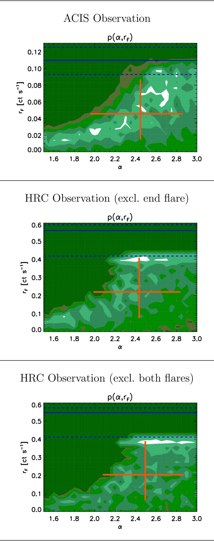
Figure 7.— Joint probability distributions $p(\alpha,r_{F})$ of the power-law flare-activity index $\alpha$ and the average contribution of flares to the observed event rate, $r_{F}$, for quiescent emission during the ACIS-S and HRC-I observations. The horizontal (blue) line near the top of each plot marks the total quiescent event rate with its $1\sigma$ uncertainty range denoted by the dashed lines. The complex contours below that enclose 68%, 90%, and 95% probabilities for $p(\alpha,r_{F})$, with the large cross locating the mean values of $\alpha$ and $r_{F}$ and the arms signifying the $1\sigma$ confidence ranges. Although it can be seen that the probability distributions are more complex than simple ellipses, on average roughly half the total quiescent emission can be ascribed to microflaring based on the ratio of $r_{F}$ and $r_{tot}$.

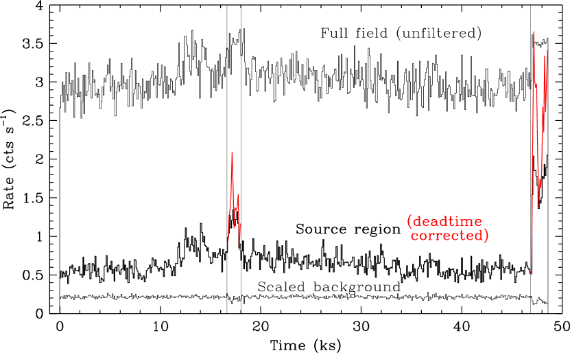
Figure 8.— Light curves of the HRC observation, with 100-s binning. Zero time corresponds to the beginning of the observation on 2007 May 28 at 4:19:18 UT. Thin vertical lines mark flare intervals, and the red traces within those intervals denote event rates after approximate corrections for deadtime due to telemetry saturation. The lowest curve is from the background region in Fig. 3 and is scaled for the area of the source region. The microflaring analysis excludes the large flare at the end (after time=46842 s). Exclusion of the small flare between times 16642 and 18042 s has little effect on the analysis.

A large flare occurred near the very end of the observation, exceeding the telemetry limit of $\sim$3.5 cts s^-1 and leading to a loss of events despite some buffering capability. Because of the limitations of the Next-In-Line mode, the deadtime can not be determined directly, but the flare intensity was at least a factor of 4 higher than the quiescent rate and probably close to a factor of 10 (see below). Some lesser flaring at 3 or more times the quiescent rate was observed earlier in the observation, and a coincidental dip in the telemetered background rate indicates that the total event rate exceeded telemetry capacity during that time. Telemetry buffering appears to have preserved all the events during a few prior periods (between $\sim t=12$ and 14 ks) when the rate briefly exceeded 3.5 cts s^-1.

Note that the upper curve in Fig. 8 plots the event rate for unfiltered full-field data, which is most relevant for comparisons with the telemetry limit. The source and background light curves are for filtered data. Standard filtering reduces the HRC-I background by 25-30% with a loss of $\sim$2% of valid X-ray events. Assuming that the true background rate is constant, one can derive the detector livetime during the flares by dividing the measured background rate by the true rate (derived from non-flare periods). The red traces in Fig. 8 plot the deadtime-corrected source rate during the two flares, with a statistical accuracy of $\sim$10% for the 100-s bins. Because many events during the large flare were lost, and those that remain may have incorrect times, we exclude the flare from our microflaring analysis. Lost events during the moderate flare near the middle of the observation may have affected the results so we repeated the analysis after excluding 1.4 ks around $t\sim 17$ ks.

In both cases, we see in Fig. 7 that the HRC-derived joint probability distribution $p(\alpha,r_{F})$ is grossly similar to that determined from the ACIS data, but there are some important differences. First, at the 90% confidence level, we can rule out $\alpha<2$, since we find that $1.99<\alpha<2.84$ (when excluding the large flare) and $2.08<\alpha<2.87$ (excluding both flares). More importantly, given that $p(\alpha)$ provides a rather poor summary of the complex 2-D $p(\alpha,r_{F})$ distribution, the broad correlation found between $r_{F}$ and $\alpha$ with ACIS data is now resolved into two major components in the probability distribution: one with $\alpha\approx 1.8$, similar to the solar case, corresponding to a low value of $r_{F}\lesssim 0.1$ ct s^-1, and another where the observed source counts are almost entirely dominated by flaring plasma, with $r_{F}\approx 0.4$ ct s^-1, and $\alpha\approx 2.5$.

This bimodal distribution is an indication that the model adopted for fitting, that of flare intensities distributed as a power-law with a single index, is too simplistic. The true flare distribution may be a broken power-law or another more complex form that requires consideration of local plasma conditions such as density, composition, and emissivity. For example, the correlation between energy deposition and X-ray emission may break down for small flares. These data thus provide the first concrete hint that different types of processes occur on late type stars than occur on the Sun, where the existence of a single power-law spanning at least 6 orders of magnitude in flare energies (from $10^{26}$ to $10^{32}$ ergs) has been well established (Aschwanden et al., 2000).

7. TEMPORAL ANALYSIS OF THE ACIS FLARE

Having completed discussion of the HRC observation, we return to the ACIS data. As seen in Fig. 9, the X-ray count rate during the flare increased by over a factor of 100 from its quiescent level. The increase in luminosity is a factor of $\sim 200$, and as noted in §5.2, observations of such large flares are quite rare. Observations of dMe stars with simultaneous X-ray and optical coverage are also uncommon but include: BY Dra with EXOSAT (de Jager et al. 1986); UV Ceti with EXOSAT and ROSAT  (Butler et al. 1986; Schmitt, Haisch, & Barwig 1993); EQ Peg with EXOSAT and ROSAT  (Butler et al. 1986; Katsova, Livshits, & Schmitt 2002); Proxima Cen with XMM-Newton (Güdel et al. 2002a); and EV Lac with Chandra (Osten et al. 2005).

In the two-ribbon solar flare model, magnetic reconnection energizes electrons in the corona that are then accelerated into the chromosphere where they heat and ionize plasma that explosively expands into the corona in the process of “chromospheric evaporation.” The multi-MK plasma then cools as it emits soft X-rays. At the beginning of the flare, synchrotron radio emission is produced as electrons spiral along the magnetic field lines and nonthermal bremsstrahlung is emitted as the electrons crash into the chromosphere at the magnetic field footprints. Optical emission is closely correlated with the nonthermal hard X-ray ($E>10$ keV) emission in solar flares (Hudson et al., 1992) and is often used as a proxy for the latter. Nonthermal flare emission is orders of magnitude weaker than the soft X-ray thermal emission and has been observed tentatively only once in another star, during a superflare in the active binary II Pegasi (Osten et al., 2007).

Soft and hard X-ray light curves are often related by the Neupert effect (Neupert, 1968). Nonthermal hard X-ray (and optical) emission traces the rate of electron energy deposition in the chromosphere, while the soft X-ray emission is approximately proportional to the cumulative thermal energy transferred to the flare plasma by the electrons, at least during the beginning of the flare before significant cooling has occurred. The time derivative of the soft X-ray light curve is therefore proportional to the hard X-ray light curve. Originally observed in solar flares, the Neupert effect (using optical or radio emission in lieu of hard X-rays) has also been observed in a few stars, including AD Leo (Hawley et al., 1995), Proxima Cen (Güdel et al., 2002a), and probably II Peg (directly in hard X-rays; Osten et al. 2007).

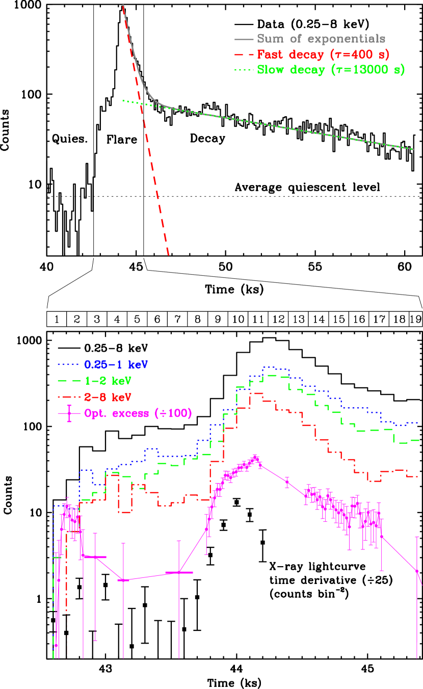
Figure 9.— X-ray light curve of the flare and its decay (top) and detail of the flare in different energy ranges (bottom); a slightly less restrictive spatial filter was used to include more counts for the bottom panel. Bin size is 100 s (20.5 s for optical in bottom panel). The pre-flare quiescent count-rate average has been subtracted from the optical data. The three data points near $t=43$ ks with wide bars in the optical curve represent average values over the indicated time intervals; gaps are dither-induced dropouts (see §4.1). The bottom-most curve traces the time derivative of the full-range (0.25–8 keV) X-ray light curve during the main flare. Beyond $t=44.2$ ks (the flare peak) the derivative is negative. Prior to the main flare the statistics are poor, but the derivative light curve seems to peak roughly in concert with the initial optical flare at $t\approx 42.7$ ks, as one would expect for the Neupert effect. The 1–19 bar across the top of the bottom panel refers to the 150-s bins used in Figs. 10 and 11.

The Ross 154 flare has two subphases: an initial count-rate rise of a factor of ten over a period of $\sim$500 s followed by a $\sim$500-s plateau, and then the main flare with another ten-fold rise. Both the initial and main flares are accompanied by optical flares (see Fig. 9 and note that the pre-flare quiescent average of $28446\pm 264$ cts bin^-1 has been subtracted from the optical data). In the initial flare, the optical signal rises abruptly to its peak (within $\sim$50 s) while the X-ray signal continues to rise after the optical flare has started to decline. Although the statistics are limited, this behavior is consistent with the Neupert effect described above, in which the optical signal is proportional to the time derivative of the X-ray signal until the X-ray peak is reached and plasma cooling takes over.

In the main flare, the optical and X-ray light curves roughly mirror each other. This is particularly true for the harder X-rays (above 2 keV), which peak $\sim$100 s before the softer X-rays, in concert with the optical light curve. The X-ray and optical light curves also begin their rise at about the same time, but the optical signal increases more quickly at first and then slows its rise to the peak. In this case, there is no simple Neupert effect, as the optical emission continues to rise even after the X-ray derivative has started falling. One possibility is that magnetic reconnection continues after the initial impulse, or perhaps conductive heating of the chromosphere by the flare maintains optical emission while the flare decays. A significant minority of large solar flares do not show a Neupert effect, and a similar mix of flare behaviors is seen on other stars (e.g., Proxima Cen; Güdel et al. 2004).

7.1. Size and Density Estimates

Although detailed dynamical and structural modeling of the flare on Ross 154 is beyond the scope of the present paper, simple geometric arguments can be used to derive rough estimates of the size of the flaring volume and the plasma density within it. We focus on the main flare event, which occurs on three time scales. First is the rise of the flare ($\tau_{rise}\approx 500$ s) followed by its decline, which can be modeled as the sum of a fast ($\tau_{fast}\approx 400$ s $e$-folding time) and slow ($\tau_{slow}\approx 13000$ s) exponential decay. This double-exponential decay is often seen in stellar flares (e.g., Osten & Brown 1999; Güdel et al. 2004; Reale et al. 2004) and is also similar to the behavior seen in large solar flares, in which a steady active region undergoes a strong magnetic reconnection event resulting in an intense flare, and is followed by an arcade of reconnected loops that slowly decay (e.g., the Bastille Day flare, see Aschwanden & Alexander, 2001). Such a scenario is also supported by the temporal analysis of §6 that finds the apparently quiescent phase likely composed of a significant amount of microflaring emission, and by spectral analysis (Table 2) which shows that active-region emission persists throughout the duration of the observation at approximately the same temperature as found for the pre-flare quiescent emission ($\sim 5$ MK).

Together with the previously derived temperatures and emission measures, the observed flare rise time and the decay time scales can be used to determine the sizes and densities of the emitting plasma. When conduction losses dominate the flare, the decay time scale can be approximated (see e.g., Winebarger, Warren, & Seaton, 2003) by

$$\tau_{C}=\frac{4\times 10^{-10}n_{e}L^{2}}{T^{5/2}}\;\;{\mathrm{(cgs)}}\,,$$ (1)

where $n_{e}$ is the electron density, $L$ is the length scale over which the plasma is distributed (the flaring loop half-length), and $T$ is the measured temperature. Given that the emission measure $EM\approx\frac{1}{2}n_{e}^{2}L^{3}$ for a hemispherical volume of radius $r=\frac{2L}{\pi}$, we can simultaneously solve for $n_{e}$ and $r$ by identifying the observed decay time scale with $\tau_{C}$. Similarly, when radiative losses dominate, the decay time scale is given by

$$\tau_{R}=\frac{3kT}{n_{e}\Lambda(T)}\,,$$ (2)

where $\Lambda(T)$ is the intensity per emission measure (in erg cm³ s^-1), obtained here combining line emissivities from ATOMDB (v1.3.1; Smith et al. 2001b) and continuum emissivities from SPEX (v1.10; Kaastra et al. 1996) with PINTofALE (Kashyap & Drake 2000) while using the fitted element abundances. As above, the plasma density $n_{e}$ and the radius of the emitting volume $r$ can be derived from the measured temperature $T$ and emission measure $EM$, after identifying the observed decay time scale with $\tau_{R}$.

At the temperatures typical of flares, $\Lambda(T)\propto T^{1/2}$ and so $\tau_{R}/\tau_{C}\propto T^{3}$. Conduction losses thus dominate during the early (hotter) part of the flare, while radiative cooling dominates the later phase. We compute estimates of the flare volume, plasma density, and loop sizes as follows:

1. Flare Rise: The sound speed in a plasma at temperature $T$ is $c_{s}=\sqrt{kT/\mu m_{p}}$, where $m_{p}$ is the proton mass and $\mu$ is the average plasma particle mass coefficient ($\sim 1/2$ in a fully ionized plasma). The rise time of a flare is generally due to the time it takes for evaporated chromospheric material to fill the flare volume. For the simplest case of impulsive heating and a single loop, the rise time equals $L/c_{s}$, and from this we can estimate the length scale of the flaring volume as $L\sim 4\,\times\,10^{10}$ cm, or $\sim 3\,R_{*}$, where $R_{*}\approx 0.20\,R_{\odot}$ is the radius of the star (cf. Ségransan et al., 2003). Because $L\propto\sqrt{T}$, this result is only weakly sensitive to uncertainties in the flare temperature and provides a firm upper limit. In reality, the heating may be non-impulsive so that evaporation continues to fill the loop for longer than $L/c_{s}$. The flare is also likely to occur in a complex loop arcade, in which the rise time is dominated by the successive lighting up of adjacent loop tubes (Reeves & Warren, 2002; Reeves et al., 2007). Solar loops have been modeled using hundreds of such strands, each lighting up a few seconds after the previous one; the typical velocities of the propagation of the sideways disturbance is $\sim\frac{1}{10}$ the sound speed (Reeves & Warren, 2002). With plausible assumptions regarding the geometry, this suggests typical flaring length scales of $L\sim 4\,\times\,10^{9}$ cm. More accurate calculations require the use of the known decay timescales (see below).

2. Initial Decay:

   As noted above, temperatures in excess of $43$ MK occur near the flare peak, and at such high temperatures, conductive loss is an important factor in the evolution of the flare intensity. Setting the observed decay timescale ($\tau_{fast}=400$ s) to match the conductive decay timescale ($\tau_{C}$) in equation 1 and using the observed flare emission measure ($EM\approx\frac{1}{2}~{}n_{e}^{2}~{}L^{3}$), we derive a plasma density $n_{e}\sim 1.6\,\times\,10^{12}$ cm^-3 and loop size $L\sim 3\,\times\,10^{9}$ cm (corresponding flare volume of diameter $\sim 3.5\,\times\,10^{9}$ cm), in good agreement with the size derived from the flare rise time assuming an arcade of loops. Uncertainties on these results are large, however, because of the $L\propto T^{5}/EM$ relationship and the large uncertainty (particularly on the high side) for the flare temperature.

   The expected radiative decay timescale for the derived plasma density is $\tau_{R}\approx 560$ s, which is similar in magnitude to $\tau_{C}$. Equating the two decay timescales (see van den Oord et al. 1988; their equation 18), we estimate the loop semi-length as

   $$L\approx 2.5\times 10^{-19}~{}\frac{EM}{T^{3.25}}\frac{1}{N_{l}\alpha^{2}}~{}{\rm cm}\,,$$

   where $N_{l}$ is the number of loops and $\alpha$ is the ratio of the loop diameter to its length, and where we have adjusted the coefficient by a factor of 0.7 to account for the change in radiative power given the measured abundances. Assuming $N_{l}=1$ and $\alpha=0.1$, we find $L\approx 10^{10}$ cm, greater than the estimate derived above. Modeling the flare decay more generally as a quasi-static cooling (van den Oord & Mewe 1989; their equation 15) results in a lower estimate of $L\approx 3\times 10^{9}$ cm, matching the original simple estimate, again assuming a single flaring loop with a constant cross-section, and $\alpha=0.1$.

3. Radiative Decay: As the flaring plasma cools, conduction losses decrease in importance and radiative losses start to dominate ($\tau_{R}<<\tau_{C}$). In the solar case, this phase coincides with the emergence of arcades of post-flare loops defined by the reconnected magnetic fields that cover approximately the same area as the pre-flare active region. Using equation (2), $\tau_{R}=\tau_{slow}=13000$ s, $T\approx 22$ MK ($kT=1.9$ keV), the observed decay-phase emission measure ($2.7\times 10^{51}$ cm^-3), and tabulated values for $\Lambda(T)$, we derive a hemispherical volume of radius $r\sim 7\,\times\,10^{9}$ cm filled with a plasma of density $n_{e}\sim 4\,\times\,10^{10}$ cm^-3. This is a robust result, as $L$ is fairly insensitive to temperature ($L\propto(EM/T)^{1/3}$). For comparison, the pressure scale height during this phase, given by $kT/(\mu m_{p}g)$ and with the gravitational acceleration $g$ calculated at the stellar surface assuming $M_{*}=0.20M_{\odot}$, is $\sim 2.6\times 10^{10}$ cm, and an arcade of magnetically confined loops that are one-quarter this height is quite plausible.

   Note that Reale, Serio, & Peres (1993; see also Reale et al. 2004) have developed a modeling method that fits hydrodynamically evolving loops to the observed light curves. Based on simulations, they derive a scaling law to determine the loop semi-length based on the initial temperature of the flare and the decay time scale,

   $$L\approx\tau_{decay}\frac{\sqrt{T/10{\rm[MK]}}}{120f(\zeta)}\,{\rm 10^{8}\,cm}\,,$$

   where $f(\zeta)>1$ is a non-dimensional correction factor that takes into account whether heating is present during the decay and $\zeta$ is the slope of the decay path in a density-temperature diagram. Note that $\zeta\approx 1.2$ here (see §7.2 below). Using this scaling law, we derive a loop semi-length $L\sim 7\times 10^{8}\frac{1}{f(\zeta)}$ cm during the fast decay. Extrapolating to the slow decay phase, we derive $L\sim 2\times 10^{10}\frac{1}{f(\zeta)}$ cm. The latter is consistent with the estimates derived above, but the former greatly underestimates the length scales involved. Note that modeling this decay as quasi-static cooling (van den Oord & Mewe, 1989) results in an estimate of the loop semi-length $L\approx 3\times 10^{11}$ cm, which is greater than all other estimates as well as greater than the coronal pressure scale height. We thus conclude that the slow decay is not well explained by quasi-static cooling, and that the simple picture of a single hydrodynamically evolving loop is too simplistic to explain the characteristics of this flare. A detailed hydrodynamic modeling of this flare is in progress.

4. Active Region: In quiescence (i.e., prior to the flare), the active region(s) on the star cover an area $\approx 50\pm 13$% (Johns-Krull & Valenti 1996) of the stellar surface. Despite the dynamic nature of an active region, based on solar observations, we may approximate it as a stationary steady state loop in radiative equilibrium (e.g., Rosner, Tucker, & Vaiana 1978 [RTV]). In such a case, the temperature $T$, pressure $p\approx 2n_{e}kT$, and the loop length $L$ obey the scaling law

   $$T=\kappa~{}(pL)^{\frac{1}{3}}\,,$$ (3)

   where the proportionality constant is estimated to be $\kappa\approx 1.4\,\times 10^{3}$ in the case of the Sun. The value of $\kappa$ is dependent on the assumed estimate of the radiative loss function. For the case of Ross 154, we estimate that $\kappa$ is reduced by a factor of $2.05\pm 0.20$. The emission measure of such a plasma is given by

   $$EM=n_{e}^{2}V\approx n_{e}^{2}(f4\pi R_{*}^{2}L)\,,$$ (4)

   where $f$ is the fraction of the stellar surface covered by active regions. For $f=0.5$, and the measured emission measure of the quiescent emission at $T=5.3$ MK ($kT=0.46$ keV), we find loop lengths $L\approx 4\times\,10^{10}$ cm. This is much larger than both the loop sizes estimated above and the pressure scale height at this temperature ($\sim 6\times 10^{9}$ cm). The latter violates the RTV assumption of a $\sim$constant pressure environment, and therefore we conclude that the active region loops are probably not in a stationary state. $L$, however, is proportional to $\kappa^{6}T^{4}/EM$, and at the assumed temperature $\kappa$ is approximately proportional to $T^{-2}$ so that $L\propto T^{-8}/EM$. A 10% uncertainty in $T$ therefore leads to an uncertainty of $\sim 2.5$ in $L$.

The size and density estimates derived above are all subject to significant uncertainties, because of assumptions regarding geometry (arcade versus single loop for the Flare Rise, low-lying stationary loops for the Active Region) or uncertainties in the fitted temperatures (particulary in the Initial Decay analysis, but also for the Active Region and Radiative Decay calculations). Results from the various flare analyses are reasonably consistent but we hesitate to interpret them in more detail.

7.2. Color-Intensity Evolution

Detailed spectral analysis (e.g., Table 2) can only be carried out over durations long compared to the time scale over which the flare evolves; analyses over shorter durations result in large errors on the fit parameters because of inadequate counting statistics. We therefore track the evolution of the hardness ratio of the flare as a means to study the evolution of the flare plasma. This evolution is shown in a color-intensity plot (Figure 10), where the color $C$ is the log of the ratio of counts in the soft (S; $0.25-1$ keV) and hard (H; $2-8$ keV) passbands and the intensity $r$ is the combined count rate in those two bands. We compute the hardness ratios and their errors using the full Poisson likelihood in a Bayesian context (Park et al. 2006). This method allows us to determine the error bars accurately even in the low-count limit, and to explicitly account for and incorporate the systematic uncertainty inherent in a specific choice of time-bin size $\delta t$ and time-start phase by considering all possible choices of phase (via cycle-spinning) and bin sizes (via marginalization). The resulting track of the flare is shown in Figure 10, where darker shades represent a longer time spent by the source in that part of the color-intensity space and the fuzziness of the shading reflects the statistical error in the calculation.

Also shown on the plot are a set of line segments marking the evolutionary track of the flare for the specific time-bin size $\delta t=150$ s, and a pair of model grids computed for different values of emission measure that bracket the observed flare intensities ($EM=0.5-15\times 10^{52}$ cm^-3). The grids are computed with the PINTofALE package (Kashyap & Drake 2000) using atomic emissivities obtained with the CHIANTI v4.2 package (Young et al. 2003) and ion balance calculations by Mazzotta et al. (1998).

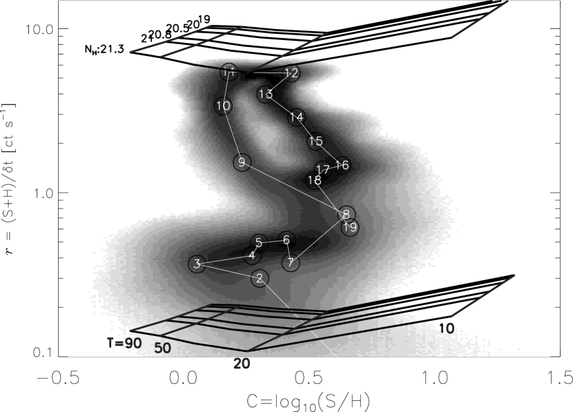
Figure 10.— Color-intensity evolution of the flare, obtained by averaging cycle-spun images at various bin sizes ranging from 40 s to 400 s. The density plot is made by sampling from the posterior probability distribution of the color $C$ (the log of the hardness ratio $S/H$) computed from the binned data points for various bin sizes and is also cycle spun to include the effects of varying the phase of the binning. Data points obtained for a light curve constructed for a bin size of 150 s (see Fig. 9) are marked on the plot and connected by the solid white lines to trace the evolution of the source. A clear pattern in the flaring plasma evolution can be seen, first rising in temperature and intensity, softening at the peak, and then decaying in temperature and intensity. Also shown are grids corresponding to an optically-thin thermal emission model calculated for two different emission measures, $1.5\times 10^{53}$ cm^-3 for the upper one, and $5\times 10^{51}$ cm^-3 for the lower one. The grids are computed for temperatures $T=10$, 20, 50, and 90 MK and for column densities $\log{N_{H}}=19$ to 21.3. Spectral fits to the summed data result in values of $N_{H}$ that are consistent with zero, however, from comparing the model thermal emission grids with the color-intensity values for bin 3, instances of large $N_{H}$ cannot be ruled out.

A number of notable features are present in the evolutionary track of the flare. First, there is a sharp initial hardening of the spectrum coincident with the onset of the small initial optical flare (bins 1–3; see Figures 9 and 10). We identify this with the initial onset of the reconnection event that generates a non-thermal hard X-ray flare. The spectrum at bin 3 appears to be either non-thermal so that the EM grids do not apply, or else has a high temperature and a very high column density ($N_{H}>5\times 10^{20}$ cm^-2) that might be associated with a coronal mass ejection. There are, however, too few counts for a spectral-fitting analysis to distinguish between these possibilities, and the uncertainty ranges for $r$ and $C$ may be large enough to permit a less interesting low-density thermal explanation. Thereafter, the plasma thermalizes, causing the spectrum to become softer and the intensity to rise because of increased radiative loss (bins 3-8). At this point, the main reconnection event occurs, leading to a large flare that increases in intensity and spectral hardness (bins 8-11), before heat input ceases and the plasma decays back to lower intensities and softer spectra (bins 12-19) during the rapid conductive-decay phase of the flare.

Figure 11.— The evolutionary track of the main flare in Temperature–Emission-Measure space. A plasma model assuming the same abundances as determined with the spectral analysis of the flare counts (Table 2) and a low column density ($N_{H}=10^{19}$ cm^-2) was used to convert the colors and intensities of Figure 10 to temperature and emission measure. The bin numbers corresponding to the time of the flare (see Figure 9) are shown, connected by dotted lines.

The color-intensity track in Figure 10 can be converted to a locus of evolution in Temperature and Emission Measure ($T-EM$) space if the absorption column $N_{H}$ and the plasma abundances are fixed throughout the duration of the flare. We adopt a low column density of $N_{H}=10^{19}$ cm^-2 (any value below $\sim 10^{20}$ cm^-2 has no significant effect) and the fitted flare abundances (Table 2) to compute the temperature from the color and the emission measure from the intensity (Figure 11) for the main flare (bins 8–19). If we further assume that the flare volume does not change over this time, then the $EM$ axis tracks changes in $n_{e}^{2}$. From the $T-EM$ track, we see this sequence of events: first, the temperature increases rapidly, followed by a rapid increase in density, as the evaporated chromospheric material fills the flare volume (bins 8–11). Then, the plasma starts to cool rapidly as the density reaches its peak, and eventually returns to the pre-main-flare environment.

During this cooling phase (bins 12–19), $EM\propto T^{2.4\pm 0.7}$. Assuming that the flare volume does not vary, this means that $n_{e}\propto T^{\zeta}$ where $\zeta\approx 1.2\pm 0.35$ (see Radiative Decay discussion in §7.1). This value of $\zeta$ corresponds to an intermediate level of heating occuring during the flare, similar to the flare observed on Proxima Cen (Reale et al. 2004). The flare evolution, however, is seen to be highly complex; looking at a shorter portion of the cooling phase (bins 13–16), the index $\zeta\approx 0.6\pm 0.1$, which is indicative of greater heat deposition. This continuous heating may be a manifestation of a flare arcade, as is often seen during solar flares (e.g., Reeves et al. 2002). Detailed hydrodynamical modeling of the flare arcade is necessary in order to definitively establish the flare environment.

8. MASS LOSS AND STELLAR WIND CHARGE EXCHANGE HALO

Mass-loss rates of a few times $10^{-10}$ to more than $10^{-5}$ ${M}_{\odot}$ yr^-1 have been measured for many stars using a variety of methods based on P Cygni profiles, optical and molecular emission lines or absorption lines, and infrared and radio excesses (Lamers & Cassinelli, 1999). All those measurements, however, are of strong winds from massive OB and Wolf-Rayet stars or cool red giants and supergiants. For comparison, the solar mass-loss rate ($\dot{M}_{\odot}$) is only $\sim 2\times 10^{-14}$ ${M}_{\odot}$ yr^-1. Because of their frequent large flares, it might be expected that dMe stars would have comparable or larger mass-loss rates, and because of their sheer numbers, M dwarfs would then contribute substantially to the chemical enrichment of the ISM.

It was not until very recently that measurements of the modest stellar winds from low-mass stars became feasible, beginning with $\alpha$ Cen AB ($\dot{M}$$=2$$\dot{M}_{\odot}$) and Proxima Cen ($\dot{M}$$<0.2$$\dot{M}_{\odot}$) (Wood et al., 2001). Over a dozen late-type mostly main-sequence stars have now been studied with measured mass-loss rates ranging from 0.15 to 100 $\dot{M}_{\odot}$ (Müller, Zank, & Wood, 2001; Wood et al., 2002, 2005). Those studies have revealed that mass-loss rates are roughly proportional to a star’s X-ray luminosity per unit surface area, except for M dwarfs, which surprisingly have much lower mass-loss rates than predicted by that relation.

All the late-type-star measurements were made using the Hubble Space Telescope Goddard High Resolution Spectrometer to measure H Ly$\alpha$ absorption profiles. To summarize, the interaction of a stellar wind with a partially neutral ISM, primarily in charge exchange (CX) collisions between stellar-wind protons and neutral H atoms from the ISM, creates a region of enhanced neutral H density, or ‘hydrogen wall,’ in the star’s astropause (analog of the Sun’s heliopause). The resulting density enhancement leads to excess absorption in the wings of the star’s Ly$\alpha$ line, which can be measured and modeled to deduce the total stellar mass-loss rate.

At the time the first of those results were published, another more direct but less sensitive stellar-wind detection method, also based on charge exchange processes, was proposed by Wargelin & Drake (2001). This method searches for X-ray emission from the very small fraction of metal ions in the stellar wind, which charge exchange with neutral gas streaming into the astrosphere from the ISM. In CX collisions of the highly charged wind ions, especially H-like and fully ionized O, an electron from a neutral H or He atom is captured into a high-$n$ level of the metal ion (usually $n=5$ for O) from which it then radiatively decays, emitting an X-ray. Although coronal X-ray emission from a star is roughly $10^{4}$ times as bright as its stellar-wind CX emission, the latter is emitted throughout the astrosphere with a distinctive spectral signature which permits both spatial and spectral filtering to be applied. This X-ray CX method was first applied to a Chandra observation of Proxima Cen, resulting in a null detection of the CX halo and an upper limit for the mass-loss rate of 14$\dot{M}_{\odot}$ (Wargelin & Drake, 2002), compared to an upper limit of 0.2$\dot{M}_{\odot}$ derived using the Ly$\alpha$ method (Wood et al., 2001). In the remainder of §8 we apply the CX technique to Ross 154, explain why we are ultimately unable to deduce even an upper limit for its mass-loss rate, and discuss future prospects for this detection method.

8.1. CX Analysis

As described by Wargelin & Drake (2002), the total rate of X-ray emission from a star as the result of CX of a particular species of ion is simply equal to the production rate of that ion in the stellar wind, either from its creation in the corona or as the result of the CX of a more highly charged ion state. As an example, the emission rate of He-like O X-rays is equal to the sum of the creation rate of H-like O ions and the creation rate of bare O ions, which eventually charge exchange to create H-like ions. Oxygen is the most abundant metal ion in stellar winds, and with a coronal temperature of 0.46 keV ($5.3\times 10^{6}$ K) nearly all of the O ions in Ross 154’s wind are fully stripped O⁸⁺ (Mazzotta et al., 1998). Those ions emit O VIII Lyman photons via CX, followed eventually by O VII K$\alpha$ emission after the ions CX a second time.

The total number of X-ray photons emitted via CX processes from oxygen ions in the Ross 154 wind and then detected by a telescope with effective area $A$ is thus equal to

$$N_{tot}=2R_{O}t\frac{A}{4\pi d^{2}}$$ (5)

where $R_{O}$ is the production rate of (fully stripped) O ions in the stellar wind, $t$ is the observation time (42620 s for the quiescent phase), and $d$ is the distance to the star (2.97 pc). The factor of 2 is because each O ion emits a H-like and then a He-like X-ray.

To calculate $R_{O}$ we consider the case in which Ross 154 has the same mass-loss rate as the Sun, $\dot{M}$$=2\times 10^{-14}$ ${M}_{\odot}$ yr^-1. Assuming the same He/H ratio as for the solar wind, 0.044, and half the metal abundance (net 0.001 relative to H), the total mass-loss rate is $6.65\times 10^{35}$ ions s^-1, of which $6.36\times 10^{35}$ ions s^-1 are protons. The ratio of O and H ions in the wind (which we assume is equal to their ratio in the corona) is equal to the product of: the coronal abundance of O relative to the solar photospheric abundance; the solar photospheric to coronal O abundance ratio (1.10; Anders & Grevesse, 1989); and O to H ratio in the solar wind ($5.6\times 10^{-4}$; Schwadron & Cravens, 2000). In the case of half-solar coronal abundances, $R_{O}$ is $1.9\times 10^{32}$ ions s^-1, and with an effective area of $\sim$320 cm² for Chandra/ACIS-S3 in the energy range for O emission ($\sim$600 eV), $N_{tot}$ is 5 counts for a 1$\dot{M}_{\odot}$ wind. If those counts could be isolated from the detector background and coronal emission, a stellar wind only a few times stronger could be detected.

8.1.1 Searching for the CX Excess

To isolate the CX emission we take advantage of its unique spectral and spatial characteristics. As noted above, oxygen is the most important element in stellar CX halos, primarily because it is the most abundant metal. It is also the highest-$Z$ element that has a large fraction of the bare and H-like ions that emit X-rays following CX; C ions are nearly abundant and even more highly ionized, but their X-ray emission is at lower energies where X-ray detection efficiency is usually poor. L-shell Fe emission may also contribute but at a lower level over a relatively broad range of energies. For these reasons we focus on O emission between 560 and 850 eV, encompassing He-like O VII K$\alpha$ ($\sim$565 eV), H-like O VIII Ly$\alpha$ (654 eV), and the high-$n$ Lyman lines (775–836 eV). Because of the moderate energy resolution of the ACIS-S3 CCD, we make our energy cuts at 525 and 875 eV.

To further enhance contrast against the coronal emission we use spatial discrimination and compare the radial profiles of the source emission during quiescence and during the flare (when the fraction of CX emission is negligible). As mentioned above and explained in more detail in §8.1.2, Ross 154’s CX emission is expected to appear around the star in an approximately symmetric shell-like halo. During the flare the observed source emission distribution will be essentially identical to the intrinsic telescope PSF because any CX emission will contribute a minuscule fraction of the total observed events. During quiescence any halo emission will, if strong enough, manifest itself as an excess relative to the the flare PSF. Although the flare and quiescent spectra are different, the energy range we use for our analysis (525–875 eV) is narrow enough that differences in the effective PSF for each phase’s emission are negligible compared to the statistical uncertainties described below.

When searching for the CX halo emission, we cannot look too close to the source centroid because the coronal emission is thousands of times stronger and completely swamps that from the halo, despite the very tight Chandra PSF. Likewise, the halo extraction region cannot be too large or the detector background will dominate the CX signal. For this observation (with its particular background, and number of quiescent and flare counts within the chosen energy band), an annulus with radii of approximately 35 and 81 pixels (corresponding to 17” and 40”, or 51 and 119 AU) provides the best sensitivity after a 5-pixel-wide box around the bright readout streak is excluded.

To compare the fraction of halo-region emission during the quiescence and flare we must know the total number of counts during each phase. This was determined from the number of counts in the readout streaks (excluding a 20-pixel-radius circle around the source and correcting for background and underlying events distributed by the telescope PSF), dividing by the fraction of the streak used (162 rows out of 206), and then dividing by the exposure time fraction for the complete readout streak, equal to 1.35% (see §4.2.1).

Using the energy range and source region described above we found $97\pm 14$ quiet counts and $200\pm 15$ flare counts, giving count fractions of $0.00285\pm 0.00044$ and $0.00367\pm 0.00032$, respectively. The net difference is therefore $-0.00082\pm 0.00054$. Equivalently, $125\pm 13$ quiet counts were expected based on the flare ratio while $97\pm 14$ counts were observed, yielding a statistically insignificant deficit of $28\pm 19$ counts. Several other combinations of energy range and annulus size were also tried, with similar results.

8.1.2 Modeling the Spatial Distribution

After obtaining the above null result for CX halo emission, we attempted to obtain an upper limit on the stellar mass-loss rate by computing how many CX events would need to be detected to obtain a statistically significant excess. This requires more detailed modeling of the expected spatial distribution of the CX emission in order to determine $f_{ann}$, the fraction of CX photons that would be detected within the chosen annulus.

Based on absorption-line spectra obtained by HST and EUVE, Ross 154 is believed to be surrounded by the ‘G cloud,’ a region of enhanced density a few parsecs in size for which Linsky et al. (2000) have derived a value of 0.10 cm^-3 for the neutral H density. The G cloud is moving roughly toward us from the direction of Ross 154, toward $l=184.5^{\circ}$, $b=-20.5^{\circ}$ (Lallement & Bertin, 1992), with virtually the same velocity (29.4 km s^-1) and direction of motion as the Local Interstellar Cloud surrounding the Sun. Given its proper motion and the radial velocity listed in the SIMBAD database (-4 km s^-1; Wallerstein & Tyagi, 2004), Ross 154 sees an ISM wind of 22 km s^-1, with the upwind side of its astrosphere pointed roughly toward the Galactic center and the viewing angle from Earth nearly aligned with the axis of its astrosphere (at an angle of $26^{\circ}$; B. E. Wood 2005, private communication).

As noted in §8, a hydrogen wall of neutral gas is expected to form on the upwind side, and it is in this region of enhanced neutral gas density that the CX emission will be most concentrated. Given the orientation of the H wall, we model it as a hemispherical shell pointed toward Earth. Outside the shell, the ISM is undisturbed, while inside the density of neutral H can be approximated (Cravens, 2000) as $n_{H}=n_{H}^{asy}e^{-(\lambda_{H}/r)}$ where $n_{H}^{asy}$ is the asymptotic density just inside the H wall, $\lambda_{H}$ is the scale for neutral H depletion near the star (from photoionization and proton-H CX), and $r$ is radial distance.

Based on the astrospheric modeling results of Wood et al. (2002) we have derived the following approximate scaling relations:

$$R_{inner} \sim 110\left(\frac{\dot{M}}{\dot{M}_{\odot}}\right)^{0.5}\mathrm{AU}$$ (6)

$$R_{outer} \sim 200\left(\frac{\dot{M}}{\dot{M}_{\odot}}\right)^{0.5}\mathrm{AU}$$ (7)

$$n_{H}^{wall} \sim 3\,n_{H}^{\,ISM}$$ (8)

$$n_{H}^{asy} \sim 0.25\,n_{H}^{\,ISM}\left(\frac{\dot{M}}{\dot{M}_{\odot}}\right)^{-0.3}$$ (9)

$$\lambda_{H} \sim 3.3\left(\frac{\dot{M}}{\dot{M}_{\odot}}\right)\mathrm{AU},$$ (10)

where $R_{inner}$ and $R_{outer}$ are the inner and outer radii of the H wall, $n_{H}^{wall}$ is the neutral H density within the wall, $n_{H}^{\,ISM}$ is the neutral H density in the undisturbed ISM (0.10 cm^-3), and all values are appropriate for the upwind direction for $\dot{M}$$/$$\dot{M}_{\odot}$$\gtrsim 1$ and relative cloud/star velocities of less than $\sim 50$ km s^-1.

The distribution of neutral He is less well understood but also less important. We assume that its density is given by $n_{He}=0.10n_{H}^{asy}e^{-(\lambda_{He}/r)}$ where $\lambda_{He}$ is approximately $1\left(\frac{\dot{M}}{\dot{M}_{\odot}}\right)$ AU. CX emission from the downwind hemisphere is roughly equal to the upwind emission but spread over such a large volume of space that we ignore it in our detectability calculations.

Detailed descriptions of the spatial emission calculations are found in Wargelin & Drake (2001, 2002). Cross sections for CT of highly charged C, N, O, and Ne ions with atomic H and associated radiative branching ratios are taken from Harel, Jouin, & Pons (1998), Greenwood et al. (2001), Rigazio, Kharchenko, & Dalgarno (2002), Johnson et al. (2000), and related references in Kharchenko & Dalgarno (2000, 2001). To summarize, the stellar wind is assumed to expand isotropically and CX with neutral gas in the astrosphere having a distribution and density described by the equations above. For bare O⁸⁺ and H, the CX cross section $\sigma_{CX}$ is $3.4\times 10^{-15}$ cm², and $3.7\times 10^{-15}$ cm² for O⁷⁺. CX with He, which is relatively unaffected by its passage from the ISM into the astrosphere (there is no ‘He wall’ density enhancement) is also included in our model. The density of each ion species is calculated numerically and its emissivity and fractional abundance computed at each step (e.g., the fraction of O⁸⁺ decreases with distance as it charge exchanges to create O⁷⁺ ions and O VIII Lyman photons). The initial composition of stellar-wind O ions is set to 95% O⁸⁺ and 5% O⁷⁺.

For modest $\dot{M}$$/$$\dot{M}_{\odot}$ (less than $\sim$20), the CX emission profile (projected on the sky and summed in annular bins around the star) rises steeply from the center and then slowly falls (see Fig. 12). The deficit of emission at small radii is because of neutral gas depletion near the star, and the falloff in X-ray CX emission at large radii occurs because highly charged ions are ‘used up’ as they CX with neutral gas, recombining into lower charge states that can not emit at X-ray energies. The CX luminosity from such winds, however, is too small for us to detect.

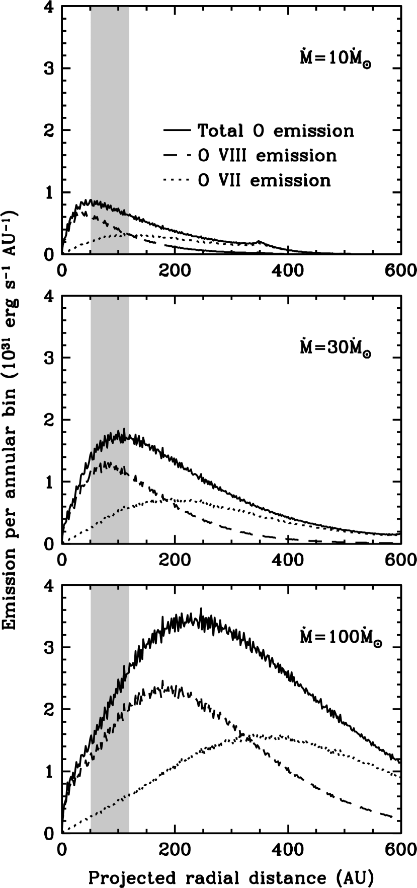
Figure 12.— Modeled radial CX emission distributions for various mass-loss rates. 100 AU corresponds to 34”. At rates above $\sim 20$$\dot{M}_{\odot}$, most emission occurs in a shell hundreds of AU from the star, and the emission observed in an annulus near the star (51–119 AU, shaded gray) becomes increasingly independent of the mass-loss rate. Emission at small radii is nearly all from H-like O⁷⁺ but at larger distances an increasing fraction of emission comes from He-like O⁶⁺ as stellar-wind ions undergo further CX collisions.

For larger mass-loss rates, the astrosphere is essentially swept clear of neutral gas ($n_{H}^{\,asy}\lesssim 0.10$; see eq. 9) so that CX emission is concentrated in the astropause in a shell around the star. When viewed from afar the emission per radial bin steadily rises from the center as the line of sight traverses an increasingly long path through the emission shell and then gradually falls at larger distances as the fraction of highly charged ions decreases. The emission shell is hundreds or thousands of AU in radius in such a case (eqs. 6 and 7), while the annulus used in our analysis extends to only 119 AU because of the limited field of the observation (and because the background per unit radius becomes too large). The fraction of total CX emission within this annulus, $f_{ann}$, therefore scales as approximately $R_{inner}^{-2}$. According to equation 6, however, $R_{inner}$ is proportional to $\dot{M}$^0.5, so $f_{ann}$ scales as $\dot{M}$^-1. Since the total number of counts detected within the annulus is given by $R_{ann}=f_{ann}R_{tot}$, and $R_{tot}$ is proportional to $\dot{M}$, $R_{ann}$ is nearly constant. Our ability to detect the CX excess therefore does not increase with $\dot{M}$ beyond $\sim$20$\dot{M}_{\odot}$, and so we are unable to find even an upper limit. In short, a CX halo provides too few counts to be detectable for small $\dot{M}$, while larger values of $\dot{M}$ produce more total emission but spread too diffusely over a larger projected area.

8.1.3 Future Prospects for CX Halo Detections

Ultimately, the limiting factor in such a search is telescope sensitivity. A large collecting area is thus essential, while detectors with better energy resolution can vastly improve the contrast of the CX signal against coronal emission and background. Microcalorimeters, such as the now-lost XRS onboard Suzaku (Cottam et al., 2005) and those planned for proposed missions such as Constellation-X (White & Tananbaum, 2003) and XEUS (Parmar et al., 2003), have resolution of a few eV and can isolate individual lines that are enhanced by CX, such as high-$n$ Lyman lines and the He-like K$\alpha$ forbidden and intercombination lines (Wargelin, Beiersdorfer, & Brown, 2008). With collecting areas roughly 10 and 100 times that of Chandra, Con-X and XEUS could respectively collect hundreds or thousands of CX counts from solar-mass-loss-rate stars in 100-ks exposures.

Such observations would permit direct imaging of the winds and astrospheres of main sequence late-type stars (i.e., stars with highly ionized winds), providing information on the geometry of the stellar wind, such as whether outflows are primarily polar, azimuthal, or isotropic, and whether or not other stars have analogs of the slow (more ionized) and fast (less ionized) solar wind streams. Enhanced emission in the relatively dense neutral gas outside the stellar-wind termination shock would indicate the size of the astrosphere and the orientation and approximate speed of the relative star-cloud motion. Neutral gas density can be inferred from the falloff of CX emission at large distances from the star, which is proportional to $1/\tau_{CX}=1/\sigma_{CX}n_{H}$, where $1/\tau_{CX}$ is the path length for a CX collision. The stellar wind velocity can also be determined from the hardness ratios of the H-like Lyman emission (Beiersdorfer et al., 2001). Although such studies are just beyond the capabilities of Chandra, future observatories will certainly provide abundant information on the stellar winds and astrospheres around nearby stars.

9. SUMMARY

In this paper we have analyzed data from two Chandra observations of Ross 154, which included one very large and a few moderate flares. Analysis of spectra from the ACIS observation reveals an enhanced Ne/O abundance ratio (relative to commonly accepted solar abundances) during quiescence and a further increase, along with overall metallicity, during the large flare. Because of severe event pileup, however, large corrections to the instrument effective area were needed and each spectral fit used only a few thousand counts, introducing significant uncertainties into the results.

Flaring behavior was studied at both low and very high intensity levels. Two moderate flares, which saturated the limited available telemetry, occurred during the HRC-I observation, and evidence for the Neupert effect was seen at the beginning of the large ACIS flare. Based on the spectral fit results and measured flare rise and decay times, we derived several physically reasonable estimates of flare and active region sizes and densities, along with information about the color-intensity evolution of the flare.

From temporal analysis of the quiescent emission during both observations we found that microflaring, which is the superposition of many low-level flares, shows a bimodal intensity-frequency distribution when modeled with a power-law distribution. Only a few other stars have been similarly studied, and our results provide the first evidence that flaring on late-type stars may follow a distribution more complex than the single power-law of the Sun. Lastly, we searched unsuccessfully for charge-exchange emission from the stellar wind, but conclude that the next generation of X-ray telescopes will be capable of such observations.

References

- Agrawal, Rao, & Sreekantan (1986) Agrawal, P. C., Rao, A. R., & Sreekantan, B. V. 1986, MNRAS, 219, 225
- Anders & Grevesse (1989) Anders, E. & Grevesse, N. 1989, Geo. Cosmo. Acta 53, 197
- Ambruster, Sciortino, & Golub (1987) Ambruster, C. W., Sciortino, S., & Golub, L. 1987, ApJS, 65, 273
- Aschwanden & Alexander (2001) Aschwanden, M. J., & Alexander, D. 2001, Sol. Phys., 204, 91
- Aschwanden & Parnell (2002) Aschwanden, M. J., & Parnell, C. E. 2002, ApJ, 572, 1048
- Aschwanden et al. (2000) Aschwanden, M. J., Tarbell, T. D., Nightingale, R. W., Schrijver, C. J, Title, A., Kankelborg, C. C., Martens, P., & Warren, H. P. 2000, ApJ, 535, 1047
- Asplund, Grevesse, & Sauval (2005) Asplund, M., Grevesse, N., & Sauval, A. J. 2005, in ASP Conf. Ser., 336, Cosmic Abundances as Records of Stellar Evolution and Nucleosynthesis, ed. T. G. Barnes III & F. N. Bash (San Francisco: ASP), 25
- Audard et al. (2000) Audard, M., Güdel, M., Drake, J. J., & Kashyap, V. L. 2000, ApJ, 541, 396
- Audard et al. (2003) Audard, M., Güdel, M., Sres, A., Raassen, A. J. J., & Mewe, R. 2003, A&A, 398, 1137
- Bahcall et al. (2005) Bahcall, J. N., Basu, S., & Serenelli, A. M. 2005, ApJ, 631, 1281
- Basu & Antia (2004) Basu, S., & Antia, H. M. 2004, ApJ, 606, L85
- Beiersdorfer et al. (2001) Beiersdorfer, P., Lisse, C. M., Olson, R. E., Brown, G. V., & Chen, H. 2001, ApJ, 549, L147
- Bensby, Feltzing, & Lundström (2003) Bensby, T., Feltzing, S., Lundström, I. 2003, A&A, 410, 527
- Bowyer et al. (1996) Bowyer, S., Lampton, M., Lewis, J., Wu, X., Jelinsky, P., & Malina, R. F. 1996, ApJS, 102, 129
- Butler et al. (1986) Butler, C. J., Rodono, M., Foing, B. H., & Haisch, B. M. 1986, Nature, 321, 679
- Carter et al. (2003) Carter, C., et al. 2003, ADASS XII ASP Conf. Series, 295, 477
- Christian et al. (1999) Christian, D. J., Craig, N., Cahill, W., Roberts, B., & Malina, R. F. 1999, AJ, 117, 2466
- Cottam et al. (2005) Cottam, J., et al. 2005, in AIP Conf. Proc. 774, X-ray Diagnostics of Astrophysical Plasmas: Theory, Experiment, and Observation, ed. R. Smith (New York: AIP), 379
- Cravens (2000) Cravens, T. E. 2000, ApJ, 532, L153
- de Jager et al. (1986) de Jager, C., et al. 1986, A&A, 156, 95
- Drake et al. (1995) Drake, J. J., Laming, J. M., & Widing, K. G. 1995, ApJ, 443, 393
- Drake & Testa (2005) Drake, J. J., & Testa, P. 2005, Nature, 436, 525
- Eggen (1996) Eggen, O. J. 1996, AJ, 111, 466
- Favata et al. (2000) Favata, F., Reale, F., Micela, G., Sciortino, S., Maggio, A., & Matsumoto, H. 2000, A&A, 353, 987
- Favata & Schmitt (1999) Favata, F., & Schmitt, J. H. M. M. 1999, A&A, 350, 900
- Feldman (1992) Feldman, U. 1992, Physica Scripta, T46, 202
- Fleming et al. (1993) Fleming, T. A., Giampapa, M. S., Schmitt, J. H. M. M., & Bookbinder, J. A. 1993, ApJ, 410, 387
- Fleming et al. (1995) Fleming, T. A., Schmitt, J. H. M. M., & Giampapa, M. S. 1995, ApJ, 450, 401
- Freeman et al. (2001) Freeman, P., Doe, S., & Siemiginowska, A. 2001, Proc. SPIE 4477, 76
- Gehrels (1986) Gehrels, N. 1986, ApJ, 303, 336
- Greenwood et al. (2001) Greenwood, J. B., et al. 2001, Phys. Rev. A, 63, 62707
- Güdel (2004) Güdel, M. 2004 A&A Rev., 12, 71
- Güdel et al. (2003) Güdel, M., Audard, M., Kashyap, V. L., & Drake, J. J. 2003, ApJ, 582, 42
- Güdel et al. (2001) Güdel, M., Audard, M., Magee, H., Franciosini, E., Grosso, N., Cordova, F. A., Pallavicini, R., & Mewe, R. 2001, A&A, 365, L344
- Güdel et al. (2004) Güdel, M., Audard, M., Reale, F., Skinner, S. L., & Linsky, J. L. 2004, A&A, 416, 713
- Güdel et al. (2002a) Güdel, M., Audard, Skinner, S. L., & Horvath, M. I. 2002a, ApJ, 580, L73
- Güdel et al. (2002b) Güdel, M., Audard, M., Sres, A., Wehrli, R., Behar, E., Mewe, R., Raassen, A. J. J., & Magee, H. R. M. 2002b, in ASP Conf. Ser. 277, Stellar Coronae in the Chandra and XMM-Newton Era, ed. F. Favata & J. J. Drake (San Francisco: ASP), 49
- Güdel et al. (1999) Güdel, M., Linsky, J. L., Brown, A., & Nagase, F. 1999, ApJ, 511, 405
- Grevesse & Sauval (1998) Grevesse, N., & Sauval, A. J. 1998, Space Science Reviews, 85, 161
- Harel, Jouin, & Pons (1998) Harel, C., Jouin, H., & Pons B. 1998, At. Data and Nucl. Data Tables, 68, 279
- Hawley et al. (1995) Hawley, S. L., et al. 1995, ApJ, 453, 464
- Heinke et al. (2003) Heinke, C. O., Edmonds, P. D., Grindlay, J. E., Lloyd, D. A., Cohn, H. N., & Lugger, P. M. 2003, ApJ, 590, 809
- Hünsch et al. (1999) Hünsch, M., Schmitt, J. H. M. M., Sterzik, M. F., & Voges, W. 1999, A&AS, 135, 319
- Hudson (1991) Hudson, H. S. 1991, Sol. Phys., 133, 357
- Hudson et al. (1992) Hudson, H. S., Acton, L. W., Hirayama, T., & Uchida, Y. 1992, PASJ, 44, L77
- Johns-Krull & Valenti (1996) Johns-Krull, C. M., & Valenti, J. A. 1996, ApJ, 459, L95
- Johnson et al. (2000) Johnson, W. R., Savukov, I. M., Safronova, U. I., & Dalgarno, A. 2000, ApJS, 141, 543
- Kaastra et al. (1996) Kaastra, J. S., Mewe, R., & Nieuwenhuijzen, H., 1996, in UV and X-ray Spectroscopy of Astrophysical and Laboratory Plasmas, eds. K. Yamashita & T. Watanabe (Univ. Acad. Press), 411
- Kashyap & Drake (2000) Kashyap, V., & Drake, J. J. 2000, Bull. Astr. Soc. India, 28, 475
- Kashyap et al. (2002) Kashyap, V. L., Drake, J. J., Güdel, M., & Audard, M. 2002, ApJ, 580, 1118
- Katsova, Livshits, & Schmitt (2002) Katsova, M. M., Livshits, M. A., & Schmitt, J. H. M. M. 2002, in ASP Conf. Ser., Stellar Coronae in the Chandra and XMM-Newton Era, ed. F. Favata & J. J. Drake (San Francisco: ASP), 515
- Kellett & Tsikoudi (1997) Kellett, B. J., & Tsikoudi, V. 1997, MNRAS, 288, 411
- Kharchenko & Dalgarno (2001) Kharchenko, V., & Dalgarno, A. 2001, ApJ, 554, L99
- Kharchenko & Dalgarno (2000) Kharchenko, V., & Dalgarno, A. 2000, J. Geophys. Res., 105, 18351
- Krucker & Benz (1998) Krucker, S., & Benz, A. O. 1998, ApJ, 501, L213
- Lallement & Bertin (1992) Lallement, R., & Bertin, P. 1992, A&A, 266, 479
- Lamers & Cassinelli (1999) Lamers, H. J. G. L. M., & Cassinelli, J. P. 1999, Introduction to Stellar Winds (Cambridge: Cambridge University Press)
- Lampton et al. (1997) Lampton, M., Lieu, R., Schmitt, J. H. M. M., Bowyer, S., Voges, W., Lewis, J., & Wu, X. 1997, ApJS, 108, 545
- Landi, Feldman, & Doschek (2007) Landi, E., Feldman, U., & Doschek, G. A. 2007, ApJ, 659, 743
- Lin et al. (1984) Lin, R. P., Schwartz, R. A., Kane, S. R., Pelling, R. M., & Hurley, K. C. 1984, ApJ, 283, 421
- Linsky et al. (2000) Linsky, J. L., Redfield, S., Wood, B. E., & Piskunov, N. 2000, ApJ, 528, 756
- Mazzotta et al. (1998) Mazzotta, P., Mazzitelli, G., Colafrancesco, S., & Vittorio, N. 1998, A&AS, 133, 403
- Müller, Zank, & Wood (2001) Müller, H.-R., Zank, G. P., & Wood, B. E. 2001, ApJ, 551, 495
- Neupert (1968) Neupert, W. M. 1968, ApJ, 153, L59
- Osten & Brown (1999) Osten, R. A., & Brown, A. 1999, ApJ, 515, 746
- Osten et al. (2007) Osten, R. A., Drake, S., Tueller, J., Cummings, J., Perri, M., Moretti, A., & Covino, S. 2007, ApJ, 654, 1052
- Osten et al. (2005) Osten, R. A., Hawley, S. L., Allred, J. C., Johns-Krull, C. M., & Roark, C. 2005, ApJ, 621, 398
- Pan et al. (1997) Pan, H. C., Jordan, C., Makishima, K., Stern, R. A., Hayashida, K., & Inda-Koide, M. 1997, MNRAS, 285, 735
- Park et al. (2006) Park, T., Kashyap, V. L., Siemiginowska, A., van Dyk, D. A., Zezas, A., Heinke, C., & Wargelin, B. J. 2006, ApJ, 652, 610
- Parmar et al. (2003) Parmar, A. N., et al. 2003, Proc. SPIE 4851, 304
- Perryman et al. (1997) Perryman, M. A. C., et al. 1997, A&A, 323, L49
- Raassen et al. (2003) Raassen, A. J. J., Mewe, R., Audard, M., & Güdel, M. 2003, A&A, 411, 509
- Read et al. (2006) Read, A. M., Sembay, S. F., Abbey, A. F., & Turner, M. J. L. 2006, Proc. “The X-Ray Universe 2005,” ed. A. Wilson, (ESA SP-604), 925
- Reale, Serio, & Peres (1993) Reale, F., Serio, S., & Peres, G., 1993, A&A, 272, 486
- Reale et al. (2004) Reale, F., Güdel, M., Peres, G., & Audard, M., 2004, A&A, 416, 733
- Reeves & Warren (2002) Reeves, K. K., & Warren, H. P. 2002, ApJ, 578, 590
- Reeves et al. (2007) Reeves, K. K., Warren, H. P., & Forbes, T.G. 2007, ApJ, submitted
- Rigazio, Kharchenko, & Dalgarno (2002) Rigazio, M., Kharchenko, V., & Dalgarno, A. 2002, Phys. Rev. A, 66, 64701
- Robinson et al. (1995) Robinson, R. D., Carpenter, K. G., Percival, J. W., & Bookbinder, J. A. 1995, ApJ, 451, 795
- Robrade & Schmitt (2005) Robrade, J., & Schmitt, J. H. M. M. 2005, A&A, 435, 1073
- Rosner, Tucker, & Vaiana (1978) Rosner, R., Tucker, W. H., & Vaiana, G. S. 1978, ApJ, 220, 643
- Saar (1994) Saar, S. H. 1994, in IAU Symp. 154, Infrared Solar Physics, ed. D. M. Rabin et al. (Dordrecht: Kluwer), 493
- Saar & Linsky (1985) Saar, S. H., & Linsky, J. L. 1985, ApJ, 299, L47
- Schmelz et al. (2005) Schmelz, J. T., Nasraoui, K., Roames, J. K., Lippner, L. A., & Garst, J. W. 2005, ApJ, 634, L197
- Schmitt et al. (1990) Schmitt, J. H. M. M., Collura, A., Sciortino, S., Vaiana, G. S., Harnden, F. R., Jr., & Rosner, R. 1990, ApJ, 365, 704
- Schmitt, Haisch, & Barwig (1993) Schmitt, J. H. M. M., Haisch, B., & Barwig, H. 1993, ApJ, 419, L81
- Schwadron & Cravens (2000) Schwadron, N. A., & Cravens, T. E. 2000, ApJ, 544, 558
- Ségransan et al. (2003) Ségransan, D., Kervella, P., Forveille, T., & Queloz, D. 2003, A&A, 397, L5
- Smith et al. (2001a) Smith, R. K., Brickhouse, N. S., Liedahl, D. A., & Raymond, J. C. 2001a, ApJ, 556, L91
- Smith et al. (2001b) Smith, R. K., Brickhouse, N. S., Liedahl, D. A., & Raymond, J. C. 2001b, Spectroscopic Challenges of Photoionized Plasmas, ASP Conference Series Vol. 247, eds. G. Ferland & D. W. Savin (San Francisco: ASP), 159
- Stuhlinger et al. (2006) Stuhlinger, M., et al. 2006, Proc. “The X-Ray Universe 2005,” ed. A. Wilson, (ESA SP-604), 937
- Telleschi et al. (2005) Telleschi, A., Gü, M., Briggs, K., Audard, M., Ness, J.-U., & Skinner, S. L. 2005, ApJ, 622, 653
- van den Oord & Mewe (1989) van den Oord, G. H. J., & Mewe, R. 1989, A&A, 213, 245
- van den Oord et al. (1988) van den Oord, G. H. J., Mewe, R., & Brinkman, A. C. 1988, A&A, 205, 181
- Wallerstein & Tyagi (2004) Wallerstein, G., & Tyagi, S. 2004, PASP, 116, 554
- Wargelin, Beiersdorfer, & Brown (2008) Wargelin, B. J., Beiersdorfer, P., & Brown, G. V. 2008, Can. J. Phys., in press
- Wargelin et al. (2004) Wargelin, B. J., Markevitch, M., Juda, M., Kharchenko, V., Edgar, R., & Dalgarno, A. 2004, ApJ, 607, 596
- Wargelin & Drake (2001) Wargelin, B. J., & Drake, J. J. 2001, ApJ, 546, L57
- Wargelin & Drake (2002) Wargelin, B. J., & Drake, J. J. 2002, ApJ, 578, 503
- Wertheimer & Laughlin (2006) Wertheimer, J. G., & Laughlin, G. 2006, AJ, 132, 1995
- White et al. (1994) White, N. E., Arnaud, K., Day, C. S. R., Ebisawa, K., Gotthelf, E. V., Mukai, K., Soong, Y., Yaqoob, T., & Antunes, A. 1994, PASJ, 46, L97
- White & Tananbaum (2003) White, N. E., & Tananbaum, H. D. 2003, Proc. SPIE 4851, 293
- Winebarger et al. (2002) Winebarger, A., Emslie, A. G., Mariska, J. T., & Warren, H. P. 2002, ApJ, 565, 1298
- Winebarger, Warren, & Seaton (2003) Winebarger, A. R., Warren, H. P., & Seaton, D. B., 2003, ApJ, 593, 1164
- Wood et al. (1994) Wood, B. E.; Brown, A., Linsky, J. L., Kellett, B. J., Bromage, G. E., Hodgkin, S. T., & Pye, J. P. 1994, ApJS, 93, 287
- Wood et al. (2001) Wood, B. E., Linsky, J. L., Müller, H.-R., & Zank, G. P. 2001, ApJ, 547, L49
- Wood et al. (2002) Wood, B. E., Müller, H.-R., Zank, G. P., & Linsky, J. L. 2002, ApJ, 574, 412
- Wood et al. (2005) Wood, B. E., Redfield, S., Linsky, J. L., Müller, H. R., & Zank, G. P. 2005, ApJS, 159, 118
- Young (2005) Young, P. R. 2005, A&A, 444, L45
- Young et al. (2003) Young, P. R., Del Zanna, G., Landi, E., Dere, K. P., Mason, H. E., & Landini, M. 2003, ApJS, 144, 135