Abstract

The cutoff version of the AdS/CFT correspondence states that the Randall Sundrum scenario is dual to a Conformal Field Theory (CFT) coupled to gravity in four dimensions. The gravitational field produced by relativistic Domain Walls can be exactly solved in both sides of the correspondence, and thus provides one further check of it. We show in the two sides that for the most symmetric case, the wall motion does not lead to particle production of the CFT fields. Still, there are nontrivial effects. Due to the trace anomaly, the CFT effectively renormalizes the Domain Wall tension. On the five dimensional side, the wall is a codimension 2 brane localized on the Randall-Sundrum brane, which pulls the wall in a uniform acceleration. This is perceived from the brane as a Domain Wall with a tension slightly larger than its bare value. In both cases, the deviation from General Relativity appears at nonlinear level in the source, and the leading corrections match to the numerical factors.

1 Introduction

The AdS/CFT correspondence provides a powerful tool to investigate the dynamics of gauge theories. In its original form, the correspondence relates a four dimensional ${\cal N}=4$ $SU(N)$ Super Yang-Mills (SYM) at large $N$ and strong coupling without gravity to a 5D theory of gravity in Anti de Sitter (AdS) space [1, 2, 3] (see [4] for a review). In this note, we will be interested in an extension of this holographic duality where gravity is also included in the 4D side. This corresponds to chopping off the AdS bulk by the presence of a (UV) brane [5, 6, 7] as in the Randall Sundrum (RS) model [8]. Hence, the gravitational dynamics of matter localized on a RS brane is dual to a 4D setup where the quantum effects of the Conformal Field Theory (CFT) are taken into account. This is a particularly convenient way for learning about the quantum effects of field theories in nontrivial gravitational backgrounds, and has already been exploited in a variety of situations ranging from cosmology [6]–[15] to Black Hole physics [16]–[31].

Here, we shall revisit the quantum effects present on the gravitational background produced by (relativistic) Domain Walls, from the new perspective offered by the correspondence. The interest for this case is that the DW represents a physical situation with a moving mirror and it may give rise to particle creation [32]–[38]. Given the similarity between this and Hawking radiation, this might shed some light on the ongoing debate concerning black holes in the Randall Sundrum scenario. As argued in [22, 23], the expectation is that the large number of fields of the CFT enhances the evaporation rate and that there should be no static solutions. However, given that the CFT is strongly coupled, it is not entirely clear that the number of states to which the BH can radiate is of order $N^{2}$ [28] (see also [29, 31]). On the other hand, the DW case is more tractable. In particular, the amount of radiation produced by the wall can be explicitly found. As a first step, in this note we will restrict our attention to the cases without particle production. As we will see, even in this case the situation is not entirely trivial. Furthermore, for the most symmetric configurations, the problem can be exactly solved in both sides of the correspondence and, hence, provides one more test of its validity.

In General Relativity (GR), the spacetime generated by a DW with a maximally symmetric worldvolume is given by the so-called Vilenkin-Ipser-Sikivie (VIS) spacetime [39, 40]. In this solution, the DW inflates at a rate $H_{0}$ determined by its tension $\sigma$ as $H_{0}=\sigma/4M_{\rm Pl}^{2}$ ($M_{\rm Pl}$ is the Planck mass) and there is a Rindler horizon. This represents a repulsive gravitational field, since test particles are repelled from the wall with an acceleration set by $H_{0}$.

In the holographic dual of the Randall Sundrum model, the DW gravitates accordingly with GR but the quantum effects from the CFT (which couples to the DW only through gravity) and their backreaction are also included. Generically, the CFT can produce two types of effects. The first is particle creation. As we will see, as long as the DW worldvolume is maximally symmetric and the spacetime has a horizon, then no CFT modes can be produced. This is related to the classic result for moving mirrors, which do not create particles of conformal fields when the mirror moves with uniform acceleration.

The other kind of effect is to modify the way how the metric responds to the source, essentially due to the trace anomaly. In our case, the DW tension $\sigma$ is effectively renormalized by an amount of order $N^{2}\,H_{0}^{3}$. As a result, one can obtain self-consistent solutions representing the spacetime produced by the DW dressed with the CFT corrections. What one finds is that the Hubble rate on the wall (and the gravitational repulsion that it produces) is larger than without the CFT.

One property of the self-consistent solutions is that they cease to exist for tension larger than a certain critical value $\sigma_{c}^{(4)}\sim M_{\rm Pl}^{3}/N$. This happens precisely when the curvature scale of the DWs becomes comparable to the cutoff, which is of order $M_{\rm Pl}/N$. Hence, for $\sigma\gtrsim\sigma_{c}^{(4)}$ the theory breaks down and the details of the UV completion are important. If one views the Randall Sundrum model as the completion, this corresponds to the transition to the regime where gravity behaves as in 5D.

The 5D dual of the dressed walls are DWs localized on a RS brane [8]. In this context, a DW is a codimension 2 brane, and exact solutions can also be easily found. The DW produces a deficit angle solely determined by its tension, $\sigma$. On the other hand, the RS brane ‘pulls’ the codimension 2 brane in an accelerated motion. As a result, and in contrast with what happens in isolation, codimension 2 branes ‘attached’ to a codimension 1 brane effectively generate a repulsive gravitational field. Hence, from the point of view of a four dimensional observer on the brane, the wall appears as an ordinary Domain Wall. As we will see, the induced metric on the brane is of the VIS form, and only differs from GR in how the Hubble rate on the wall $H_{0}$ relates to $\sigma$. Furthermore, the leading order deviation from the GR result exactly matches the one we find in the CFT side, providing one further check of the correspondence.

The fact that the DWs start behaving according to 5D gravity for tensions larger than the critical value $\sigma_{c}^{(4)}$ is slightly more involved to see, but it can be summarized as follows. In the thin wall approximation, the worldvolume curvature scale $H_{0}$ diverges when the tension approaches $\sigma_{c}^{(5)}\equiv 2\pi M^{3}$, where $M$ is the Planck mass in the bulk. This is the codimension 2 notion of critical tension (the deficit angle that it produces is $2\pi$), and it is of the same order as $\sigma_{c}^{(4)}$. Of course, the divergence in $H_{0}$ only means that sooner or later one has to resolve the wall thickness, $d$. In doing so, one realizes that $H_{0}$ becomes finite even for ‘supermassive’ walls, that is, with $\sigma>\sigma_{c}^{(5)}$. If the thickness is small enough ($d\ll\ell$) then the AdS curvature becomes irrelevant and, in the neighborhood of the DW, one of the two transverse directions is effectively compactified. Since the compactification radius is of order $d$, the effective Planck mass felt by the DW is of order $dM^{3}$, which is much smaller than the 4D Planck mass, $\ell M^{3}$. The outcome is this: for supermassive walls, $H_{0}$ is enhanced with respect to GR by a factor $\ell/d$. As it was described in [41], codimension 2 branes display precisely the same kind of behaviour when the tension becomes supercritical (they compactify one of the transverse directions and inflate as a DW). Hence, the gravitational field of localized DWs turns five dimensional when the tension becomes roughly of order $\sigma_{c}^{(5)}\simeq\sigma_{c}^{(4)}$, as expected from the CFT side.

This paper is organized as follows. In Section 2 we review the gravitational effects of Domain Walls in GR. In Section 3 we work out the self-consistent solution incorporating the CFT corrections. We discuss the 5D dual in Section 4, finding the solutions for DWs localized on the brane in Sec. 4.1 and 4.2. We also show in Sec. 4.3 how resolving the thickness allows to have supermassive DW solutions. We compare the results from the two sides of the correspondence in 4.4, and we will conclude in Section 5.

2 Domain Walls in GR

In this Section, we shall briefly review some of the properties of gravitating Domain Walls in General Relativity (GR). We shall start by the thin wall description, assuming that the wall thickness is much smaller than any other scale of the problem and treating the wall as an idealized distributional source. We comment on the case with finite thickness in Sec. 2.1.

In the thin wall approximation, the stress tensor of a Nambu-Goto Domain Wall takes the form

$$T^{DW}_{\mu\nu}=\sigma\,\delta(\xi)\;{\rm diag}\left(1,-1,-1,0\right)_{\mu\nu}$$ (2.1)

where $\sigma$ is the ‘tension’ or surface energy density, $\delta(\xi)$ is the Dirac $\delta-$function and $\xi$ represents a ‘proper’ coordinate normal to the wall, which one can always find by going to Gaussian Normal coordinates around the hypersurface defined by the DW worldvolume itself.

We shall concentrate on the DW solutions with a maximally symmetric worldvolume and with $\mathbb{Z}_{2}$ symmetry across the wall. One can easily see that this implies that the metric must admit a 3D maximally symmetric slicing, i.e., it is of the form

$$ds_{4}^{2}=d\xi^{2}+R^{2}(\xi)\;ds_{\kappa}^{2}\,.$$ (2.2)

where $ds_{\kappa}^{2}$ is the line element of a 3D Minkowski ($\kappa=0$), de Sitter ($\kappa=1$) or Anti de Sitter ($\kappa=-1$) spacetime of unit radius. From (2.2), the curvature scale of the DW worldvolume is determined by $R(0)$. Thus, we shall introduce the Hubble rate on the DW as

$$H_{0}^{2}\equiv{\kappa\over R^{2}(0)}~{}.$$

We shall consider the case when a cosmological constant $\Lambda_{4}$ is also present. With a metric of the form (2.2), the Einstein equations become

$$3M_{\rm Pl}^{2}\;\frac{\kappa-R^{\prime\,2}}{R^{\,2}} =\Lambda_{4}\,,$$ (2.3)

$$M_{\rm Pl}^{2}\;\left(\frac{\kappa-R^{\prime\,2}}{R^{\,2}}-2\frac{R^{\prime\prime}}{R}\right) =\sigma\delta(\xi)+\Lambda_{4}\,.$$ (2.4)

Integrating (2.4) around $\xi=0$ leads to the junction condition on the DW

$$K_{0}={\sigma\over 4M_{\rm Pl}^{2}}~{},$$ (2.5)

where we have introduced

$$K_{0}\equiv-{1\over 2}{\Delta R^{\prime}(0)\over R(0)}~{},$$ (2.6)

and $\Delta X$ denotes $X(\xi=0^{+})-X(\xi=0^{-})$. With this, $K_{0}$ is proportional to the (jump in the) extrinsic curvature of the wall as embedded in the 4D geometry (2.2). As we illustrate below, physically $K_{0}$ sets the scale of the accelerated motion of the DW or, equivalently, the scale for the gravitational repulsion that the DW exerts on test particles. Equation (2.5) thus summarizes the gravitational effect of a DW in GR. In the next sections, we will find deviations from this relation.

On the other hand, the curvature scale on the DW worldvolume depends on the properties of the ambient space. The curvature scale away from the wall is

$$H_{4}^{2}={\Lambda_{4}\over 3M_{\rm Pl}^{2}}~{}.$$

Hence, Eq. (2.3) evaluated at $\xi=0$ can be rewritten as

$$H_{0}^{2}=K_{0}^{2}+H_{4}^{2}~{}.$$ (2.7)

This is the familiar Gauss equation for the embedding of the DW in the ambient 4D space. It follows that in de Sitter and in flat space, the walls always inflate, while in AdS₄ only DWs with tension larger than $4M_{\rm Pl}\sqrt{|\Lambda_{4}|/3}$ do so. For inflating DWs ($\kappa=1$), the ‘warp factor’ that solves (2.3) and (2.4) is

$$R(\xi)=H_{4}^{-1}\sin\left[\sin^{-1}(H_{4}/H_{0})-H_{4}|\xi|\,\right]~{}.$$ (2.8)

which is valid for any $\Lambda_{4}$ by analytic continuation. As one can see, in these cases there is a horizon ($R(\xi)$ vanishes) at a finite proper distance from the wall.

To gain some intuition, let us briefly look at the full form of the metric for the $\Lambda_{4}=0$ case. The warp factor is

$$R(\xi)=H_{0}^{-1}-|\xi|~{},$$ (2.9)

giving what is usually referred to as the Vilenkin-Ipser-Sikivie spacetime [39, 40]. The conformal diagram for this space is shown in Fig. 1. It can be viewed as two copies of the interior of the hyperboloid defined by the DW, glued together at the DW position. The coordinate $\xi$ covers part of the Rindler patch of Minkowski, and the Rindler (or ‘acceleration’) horizon is at $\xi=\pm 1/H_{0}$.

An inertial observer in this space sees the wall moving away at a constant acceleration set by $K_{0}$ (which coincides with $H_{0}$ in this case), effectively feeling a repulsive gravitational field. In this sense, the DWs unambiguously produce a nontrivial gravitational effect even though the curvature tensor is identically zero (away from the DW) and so there are no tidal forces. For general $\Lambda_{4}$, the scale of the acceleration/repulsion is set by $K_{0}$ but the curvature of the DW worldvolume (and the presence of the horizon) depends on $\Lambda_{4}$.

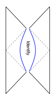
Figure 1: Conformal diagram of the Vilenkin Ipser Sikivie spacetime [42], the metric produced by a Domain Wall in otherwise flat space. The (inflating) DW corresponds to the hyperboloid represented by the blue line. The Rindler horizon (dashed line) is at $\xi=\pm 1/H_{0}$, and separates the Rindler and Milne regions.

2.1 Finite thickness walls

In the above discussion, the DW is treated as infinitesimally thin and its stress tensor as a distribution. This is not a good approximation when the curvature radius of the worldvolume is comparable to the thickness, $d$, of the wall. For our purposes, the most relevant situation when this happens is when the curvature scale provided by the gravity of the wall $K_{0}$ becomes comparable to $1/d$, that is when

$$\sigma\gtrsim{M_{\rm Pl}^{2}\over d}~{}.$$ (2.10)

For $\Lambda_{4}=0$, this corresponds to a regime of topological inflation [43], since the Hubble radius on the wall is smaller than its actual thickness, and so the DW is also inflating in the transverse direction.

We shall now show that when we take into account a nonzero $d$, then the pressure in the direction transverse to the (gravitating) DW must be nonzero, and one should replace (2.1) by

$$T_{\mu}^{\nu}={\rm diag}\left(-\rho,-\rho,-\rho,P\right)~{}.$$ (2.11)

To make this compatible with the same symmetries, $P$ and $\rho$ must depend on $\xi$ only. On the other hand, the local conservation equation on a space of the form (2.2) leads to

$$P^{\prime}+3{R^{\prime}\over R}(P+\rho)=0~{}.$$ (2.12)

We do not need to specify the actual microscopic model for the Domain Wall, as our conclusions will be model independent. The only thing we need to know is that the stress tensor of the wall obeys (2.12), and $\rho(\xi)$ is peaked at $\xi=0$, decaying exponentially fast to zero for $|\xi|\gtrsim d$, and that $R(\xi)$ is similarly a smoothed-out version of (2.8). These assumptions and (2.12) suffice to show that $P(\xi)\neq 0$ in the DW core. Note that this is independent of whether the DW is inflating or not, rather it requires only a nonzero extrinsic curvature, $R^{\prime}/R$. Hence, the presence of $P\neq 0$ can be thought to be necessary to support the accelerated motion of the DW.

In this respect, note that the thin wall approximation advocated before is slightly inaccurate. Indeed, (2.1) assumes $P=0$ even on the DW core, so that (2.12) leads to $R^{\prime}(\xi)\delta(\xi)=0$. While this is not very well defined as a distribution ($R^{\prime}$ is discontinuous at $\xi=0$), it is not clear that this should be treated as $0$ even in a distributional sense. Instead, a pressure of the form $\propto 1-\varepsilon^{2}(\xi)$, where $\varepsilon(\xi)={\rm\footnotesize sign}(\xi)$ for $\xi\neq 0$ and $\varepsilon(0)=0$, is a more accurate representation compatible with (2.12). While it remains true that this distribution vanishes when integrated with any smooth test function, it captures the fact that for gravitating thick DW solutions, it is never strictly zero at the core of the wall [44].

Actually, incorporating $P$ is also quite convenient because the (appropriately modified version of the) constraint (2.3) is a first order equation analogous to the Friedmann equation in cosmology, and it suffices to find the solutions to Einstein equations, once (2.12) is enforced. Indeed, (2.4) is a consequence of (2.12) and (2.3) as long as $R(\xi)$ is not constant.

3 Quantum effects from the CFT

In this Section we show how the quantum effects from the CFT modify the gravitational field of a Domain Wall discussed in the previous Section. We are assuming that the DW is a source external to the CFT which only interacts with it through gravity. The field produced by the DW can be simply computed from the graviton propagator dressed with the radiative corrections from the CFT. This is the procedure followed in [21] for a point particle, where a precise agreement with the brane world result of [20] was found.

In the DW case, this leads immediately to the conclusion that the CFT does not modify –at all– the field produced by DWs (to linear order in the source). This follows from the Källen Lehmann decomposition of the graviton propagator, when the CFT radiative corrections are included. The propagator has a massless graviton pole and a branch cut, which are dual to the massless graviton and the continuum of Kaluza Klein modes in the RS model. The key point is that the tensor structure of the propagator associated with the branch cut is granted to be that of a massive graviton. This couples to conserved sources as $h^{massive}_{\mu\nu}\sim T_{\mu\nu}-(T_{\rho}^{\rho}/3)\eta_{\mu\nu}$, and as it was observed in [41], this leads to a pure gauge metric perturbation. Hence, only the massless pole contributes to linear order in the graviton exchange with a Domain Wall and no correction is found even though the propagator differs from that of pure GR. In the Appendix, we illustrate it by performing a more explicit computation at 1-loop.

In the rest of this Section we shall show that, despite the previous argument, the CFT does induce a correction to the DW gravitational field that is nonlinear in the tension $\sigma$. The reason is that in the 4D side of the correspondence, the backreaction from the quantum effects of the CFT is also incorporated. This implies that the 4D metric obeys the semiclassical Einstein equations

$$M_{\rm Pl}^{2}\,G_{\mu\nu}=T_{\mu\nu}^{DW}+\langle T_{\mu\nu}\rangle^{CFT}~{},$$ (3.1)

$\langle T_{\mu\nu}\rangle^{CFT}$ is the vacuum expectation value of the stress tensor of the CFT. The solutions of (3.1) differ from GR because $\langle T_{\mu\nu}\rangle^{CFT}\neq 0$ in the VIS spacetime described in Sec. 2, essentially because the trace anomaly is nonzero in this background (see below). However, one can easily find self-consistent solutions of (3.1). One takes an ‘ansatz’ for the metric of the form (2.2), with $R(\xi)$ to be determined. Since for a maximally symmetric DW worldvolume, the form of $\langle T_{\mu\nu}\rangle^{CFT}$ can be determined without explicit reference to the actual form of $R(\xi)$, then (3.1) fixes the function $R(\xi)$ and hence the self-consistent solution.

Let us now see how to determine the energy-momentum tensor $\langle T_{\mu\nu}\rangle^{\mathrm{CFT}}$. We can always separate it as

$$\langle T_{\mu\nu}\rangle^{CFT}=\langle T_{\mu\nu}\rangle^{(0)}+T_{\mu\nu}^{\mathcal{A}}$$ (3.2)

where $T_{\mu\nu}^{\mathcal{A}}$ is the anomalous contribution while $\langle T_{\mu\nu}\rangle^{(0)}$ is tracefree and depends on the choice of vacuum. The nonzero trace ${T_{\mu}^{\mu}}^{\mathcal{A}}$ arises from the anomalous breaking of conformal invariance by the quantum effects and may be non-zero in curved spacetimes.

3.1 Absence of particle production

The state dependent contribution $\langle T_{\mu\nu}\rangle^{(0)}$ in (3.2) encodes the effects from particle creation. As we shall see, whenever there is a horizon and the wall is maximally symmetric, then $\langle T_{\mu\nu}\rangle^{(0)}=0$ and the wall does not radiate quanta of the CFT.

We will assume as before that the metric solving (3.1) allows a maximally symmetric slicing and, as such, it is of the form (2.2). In this case, the state-dependent piece $\langle T_{\mu\nu}\rangle^{(0)}$ can be completely fixed as follows. On the one hand, conformal invariance demands it to be traceless. On the other, imposing that it has the symmetries of the metric (2.2) leads to

$$\langle T_{\mu}^{\,\nu}\rangle^{(0)}=p(\xi)\,{\rm diag}\big{(}-\frac{1}{3},-\frac{1}{3},-\frac{1}{3},1\big{)}^{\nu}_{\mu}\,,$$ (3.3)

where the function $p$ depends on the DW transverse direction $\xi$ only. This kind of stress tensor (for any nontrivial dependence on the ‘Rindler’ coordinate $\xi$) implies the presence of fluxes of energy-momentum away from the DW, which is interpreted as arising from the particle creation by the moving mirror [32].

The function $p(\xi)$ is further determined from the conservation of the stress-energy tensor, which leads to $p^{\prime}/p+4R^{\prime}/R=0$, where $R(\xi)$ is the warp factor as defined in (2.2). Thus, $p(\xi)$ must be of the form $p_{0}/R^{4}(\xi)$, for some constant $p_{0}$. If the effects from the CFT do not change the asymptotic structure of the spacetime, then there is a Milne region (see Fig. 1) and hence a horizon. That is, $R(\xi)$ vanishes somewhere. Were $p_{0}$ nonzero, $\langle T_{\mu\nu}\rangle^{(0)}$ would be singular on the horizon. Thus, the only vacuum state of the CFT that is regular on the horizon has $p_{0}=0$.

Given that the 4D side of the correspondence is supposed to include the backreaction from the CFT, we should take it into account before reaching a final conclusion. In particular, we should make sure that the backreaction is not going to change the assumption that there is a horizon. Ignoring the anomalous contribution for simplicity, this reduces to finding the possible solutions of the ‘Friedmann’ equation $3M_{\rm Pl}^{2}(1-R^{\prime\,2})/R^{\,2}=-p_{0}/R^{4}$. One can easily show that if $p_{0}$ were positive, then the horizon is replaced by a naked singularity. Thus, the quantum state would be indeed singular and we should discard it as unphysical. On the other hand, if $p_{0}$ were negative then there would be regular ‘bouncing’ solutions, with flat asymptotics ($R^{\prime}(\xi)\to\pm 1$ for large $\xi$) and no horizons. However, since $p_{0}$ would be (at most) of order $N^{2}$, the curvature scale would be (at least) of order of the cutoff around the bounce. Hence, these solutions cannot be trusted and we should disregard them as well. This is confirmed by the results of Sec. 4, where no analogous solution is found.

Thus, we conclude that indeed in the regular vacuum state there is no particle creation, i.e., $p_{0}=0$. This result is confirmed by the explicit 1-loop computations [35]–[38],[50] for scalar fields, and is also expected from the analogy with moving mirrors [32]. As is well known, they only radiate to conformal fields if the motion is not uniformly accelerated, that is, if the worldvolume of the mirror is not maximally symmetric. Let us emphasize that this result should be viewed as a statement about the incompatibility of having particle production in the CFT with the amount of symmetries assumed. As such, it should remain true to all orders in the loop expansion. This will be confirmed by the computation in the dual setup of Sec. 4.

3.2 The anomalous contribution

The previous discussion implies that (for maximally symmetric worldvolume and when the Rinlder horizon is present) the only contribution to $\langle T_{\mu\nu}\rangle^{\mathrm{CFT}}$ may come from the conformal anomaly. Let us now work out this contribution. It is known that in 4D at first loop the anomalous trace is given by

$${T^{\mu}_{\mu}}^{\,\cal A}=-a\,E_{(4)}+c\,I_{(4)}+d\,\nabla^{2}{\cal R}\,,$$ (3.4)

where $E_{(4)}$ is the Euler density

$$E_{(4)} = \mathcal{R}_{\mu\nu\rho\sigma}\mathcal{R}^{\mu\nu\rho\sigma}-4\mathcal{R}_{\mu\nu}\mathcal{R}^{\mu\nu}+\mathcal{R}^{2}\,,$$ (3.5)

and $I_{(4)}=C_{\mu\nu\rho\sigma}C^{\mu\nu\rho\sigma}$ with $C_{\mu\nu\rho\sigma}$ the Weyl tensor.

The parameters $a$, $c$, and $d$ depend on the field content of the theory and are found to be

$$a = \frac{1}{360\,(4\pi)^{2}}(N_{0}+\frac{11}{2}N_{1/2}+62N_{1})\,,$$ (3.6)

$$c = \frac{1}{120\,(4\pi)^{2}}(N_{0}+3N_{1/2}+12N_{1})\,,$$ (3.7)

$$d = \frac{1}{180\,(4\pi)^{2}}(N_{0}+3N_{1/2}-18N_{1})\,,$$ (3.8)

where $N_{0}$, $N_{1/2}$, and $N_{1}$ are respectively the number of scalars, Majorana fermions and vectors of the field theory. In the particular case of RS, the field content is that of $\mathcal{N}=4$ Super Yang-Mills Theory, therefore $N_{0}=6N^{2}$, $N_{1/2}=4N^{2}$ and $N_{1}=N^{2}$, with $N$ the rank of the gauge group. With this field content, one finds

$$a=c=\frac{N^{2}}{64\pi^{2}}\,,\qquad d=0\,.$$ (3.9)

In the literature, a finite counterterm of the form $\sqrt{-g}\,R^{2}$ is often added [53, 54, 9], and it has the effect of shifting $d$ away from $0$. This term explicitly breaks conformal invariance, and we assume it is not present.

Once ${T^{\mu}_{\mu}}^{\,\cal A}$ is known, the symmetries of the problem fix the full form of $T_{\mu\nu}^{\cal A}$ as ${T_{\mu}^{\nu}}^{\,\cal A}={\rm diag}(-\rho_{\cal A},-\rho_{\cal A},-\rho_{\cal A},p_{\cal A})$ with $p_{\cal A}$ and $\rho_{\cal A}$ obeying the conservation equation ${p_{\cal A}}^{\prime}+3(p_{\cal A}+\rho_{\cal A})R^{\prime}/R=0$ and Eq. (3.4). Eliminating $\rho_{\cal A}$ in terms of $p_{\cal A}$, we are left with a first order differential equation for $p_{\cal A}$. This leads to one integration constant which as before contributes to $T_{\mu\nu}^{\cal A}$ as a ‘radiation’ term of the same form as (3.3). For the same reasons of Sec. 3.1, this has to vanish and $T_{\mu\nu}^{\cal A}$ is completely fixed. Therefore, in the semiclassical approach the quantum corrected version of the ‘Friedman’ equation (2.3) becomes (concentrating on the $\kappa=1$ case)

$$3M_{\rm Pl}^{2}\;\frac{1-R^{\prime\,2}}{R^{\,2}}=\frac{3\,N^{2}}{32\pi^{2}}\left(\frac{1-R^{\prime\,2}}{R^{\,2}}\right)^{2}-P\,,$$ (3.10)

where $P$ is the pressure of the DW in the transverse direction.

Rather than finding the exact solutions of (3.10) given a smooth profile for $P$, we shall turn to the thin wall description and restrict our attention to the extrinsic curvature $K_{0}$ and the intrinsic curvature $H_{0}$ on the DW. Technically, this can be done by integrating across the domain wall the component of (3.1) that contains the $\delta$-functions associated with the DW energy density. It can be easily reproduced from (3.10) by taking one derivative with respect to $\xi$ (and dividing by $R^{\prime}/R$) and using (2.12). Given that the warp factor $R(\xi)$ is continuous, it can be treated as a constant across the DW core. Using also that $R^{\prime}(\xi)$ has a finite discontinuity, and so the integral of any power of $R^{\prime}$ does not contribute, we find

$$K_{0}=\frac{1}{4M_{\rm Pl}^{2}}\left(\sigma+\frac{N^{2}}{12\pi^{2}}\left(3K_{0}H_{0}^{2}-K_{0}^{3}\right)\right)\,,$$ (3.11)

Hence, the only effect of the CFT is to renormalize the DW tension by an amount given in terms of the geometric invariants of the DW worldvolume, and (3.11) is all we need to solve in order to find the self-consistent solutions.

Let us emphasize that even though this is a 1-loop computation, this is all from the CFT. In general, one expects higher loop planar diagrams to contain contributions of the same order in the $1/N$ expansion and with a non-trivial dependence on the ’t Hooft coupling $\lambda=g^{2}_{YM}N$. Recall that the AdS/CFT correspondence relates this to the gravity side as $\lambda=(\ell/\ell_{s})^{4}$ where $\ell_{s}$ is the string scale and $\ell$ is the AdS curvature scale. Hence, the classical gravity description of Sec. 4 corresponds to strong coupling ($\lambda\gg 1$), so higher loops may not be negligible. However, in our case the higher loops do not contribute. The reason is that, as shown above, the CFT effects arise from the trace anomaly only. In ${\cal N}=4$ SYM, the trace and the chiral anomalies are in the same supermultiplet. Because of the non-renormalization theorem for the chiral anomaly, the trace anomaly is protected as well. Hence, (3.11) should also be valid for large $\lambda$, as the results of Section 4 will indeed confirm.

Equation (3.11) is in its most generic form, and one could use the Gauss equation (2.7) to express it in terms of $K_{0}$ and the brane curvature $H_{4}$. We shall now restrict to flat brane case, for which $H_{0}=|K_{0}|$ and

$$\frac{\sigma}{4M_{\rm Pl}^{2}}=K_{0}\left[1-\frac{1}{3}(K_{0}\ell)^{2}\right]\,.$$ (3.12)

Here we introduced

$$\ell^{2}=N^{2}/(8\pi^{2}M_{\rm Pl}^{2})~{}$$ (3.13)

merely as a short-hand notation, but as will become apparent in Section 4, $\ell$ is to be identified in the Randall-Sundrum setup as the curvature scale of the AdS bulk. Also, as we shall see shortly, $1/\ell$ plays the role of the cutoff of the theory [7]. This can also be understood along the lines of [55], as a consequence of the consistency of the theory and the fact that the CFT contains of order $N^{2}$ degrees of freedom coupled to gravity, which forces the cutoff to be $M_{\rm Pl}/N$ rather than the naively expected $M_{\rm Pl}$.

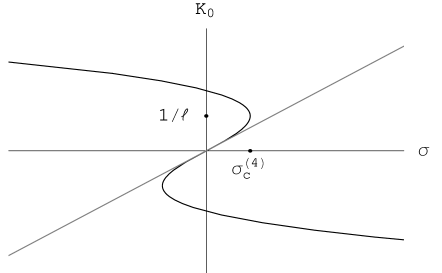
Figure 2: The extrinsic curvature of the Domain Wall $K_{0}$ as a function of its tension $\sigma$. For small enough $\sigma$, there is one branch very close to the GR result (light gray). For the other branches, $K_{0}$ is of the order or larger than the cutoff $1/\ell\sim M_{\rm Pl}/N$, and they cannot be trusted.

Equation (3.12) is cubic in $K_{0}$, and so it admits up to three branches, of which the ‘normal’ branch is the one that reduces to the GR result when the CFT is removed. As illustrated in Fig 2, for tensions below a critical value given by

$$\sigma^{(4)}_{c}={8\over 3}{M_{\rm Pl}^{2}\over\ell}={16\sqrt{2}\,\pi\over 3}{M_{\rm Pl}^{3}\over N}$$ (3.14)

two new branches of solutions appear. One of them behaves with negative effective tension (i.e., $K_{0}<0$) and is thus expected to be unstable. The other has positive effective tension, so it may be stable. One intriguing feature of these solutions is that they display a kind of self-acceleration: even for vanishing $\sigma$, the quantum corrected DW is inflating, at a rate entirely due to the CFT radiative corrections. However, just because the loop corrections are more important than the tree level effect, this suggests that this solution cannot be trusted. Indeed, given that the CFT correction is suppressed by $1/\ell$, one expects that this scale plays the role of the cutoff of the theory. But this is precisely the curvature scale of the two new branches. Thus, their actual presence is not guaranteed.

Hence, we are left only with the normal branch of solutions, the one where the radiative corrections are subdominant to the classical term (for small $\sigma$). Note that these corrections make $K_{0}$, and hence the gravitational repulsion generated by the DW, larger than in GR. Also, the difference appears only at nonlinear level in the tension. This will be exactly reproduced in the Randall Sundrum setup.

Finally, let us note that these solutions cease to exist for tensions larger than $\sigma_{c}^{(4)}$. This happens because the curvature scale $K_{0}$ becomes of order of the cutoff, $1/\ell$. Hence, the theory breaks down, that is, the solutions become sensitive to the UV completion. This is indeed what will see in the RS setup. For tensions of order $\sigma_{c}^{(4)}$ or larger, the walls start to behave in the 5D fashion.

4 Domain Walls in Randall Sundrum

As argued above, the Domain Walls dressed with the CFT radiative corrections should be dual to DWs localized on a Randall Sundrum brane [8]. This amounts to finding the metric produced by a codimension 2 brane (the Domain Wall) embedded in a codimension 1 brane (from now on, the brane). This was first discussed in [56], and here we will closely follow their derivation.

Since one can view the brane as moving with a uniform acceleration in the bulk, the solution we are looking after will contain an accelerated codimension 2 brane pulled by the codimension 1 brane. Hence, one can already expect the solution to be appropriately described in some kind of Rindler coordinates which, as we shall see, will appear naturally. As a consequence, and in contrast with isolated codimension 2 branes, the worldvolume of the accelerated ones inflates at a rate that depends on their tension. This already represents a ‘zeroth order’ check of the correspondence, since Domain Walls in 4D (with or without the CFT) do inflate at a rate sensitive to $\sigma$.

In the Randall Sundrum model, the bulk has a negative cosmological constant $\Lambda_{5}$, the brane is characterized by a tension $\tau$. Including the DW, the action is

$$S=\int d^{5}x\sqrt{-g}\;\left({M^{3}\,R_{5}\over 2}-\Lambda_{5}\right)-\int d^{4}x\sqrt{-h}\;\tau-\int d^{3}x\sqrt{-\gamma}\;\sigma\,,$$ (4.1)

where $R_{5}$ is the bulk Ricci scalar, and $h_{\mu\nu}$ and $\gamma_{\mu\nu}$ are the induced metrics on the brane and on the DW respectively.

For the time being, we will not assume any relation between the AdS curvature $\Lambda_{5}$ and the tension $\tau$ of the brane. The equations of motion for the brane (the Israel junction conditions) are

$$2M^{3}k_{\mu\nu}=T_{\mu\nu}-{1\over 3}Th_{\mu\nu}\,,$$ (4.2)

where we imposed $\mathbb{Z}_{2}$ symmetry across the brane, $k_{\mu\nu}$ is the brane extrinsic curvature and $T\equiv T^{\mu}_{\mu}$. $T_{\mu\nu}$ is the energy-momentum tensor associated with the brane and the DW,

$$T_{\mu\nu}=-\tau h_{\mu\nu}-\sigma\delta(\xi)\gamma_{\mu\nu}\,.$$ (4.3)

As before, $\xi$ is the (proper) coordinate along the brane which is orthogonal to the DW. In terms of $\xi$, the position of the DW is at $\xi=0$.

4.1 Solution

As before, we will concentrate on the solutions with the symmetries of a maximally symmetric DW, that is with a 3D maximally symmetric slicing. The (double-Wick rotated version of the) Birkhoff theorem guarantees that the most generic solution with this symmetry can be written locally as

$$ds^{2}=f(R)dZ^{2}+{dR^{2}\over f(R)}+R^{2}ds_{\kappa}^{2}\,,$$ (4.4)

where $ds_{\kappa}^{2}$ is the line element of a 3D maximally symmetric space of unit curvature radius, that is, a de Sitter ($\kappa=1$), Anti de Sitter ($\kappa=-1$) or Minkowski ($\kappa=0$) spacetime.

The form of $f(R)$ depends on the presence of bulk fields, and in their absence it is equal to

$$f(R)=\kappa+{R^{2}\over\ell^{2}}+{\mu\over R^{2}}\,.$$ (4.5)

Here, $\ell^{2}=|6M^{3}/\Lambda_{5}|$ is the AdS curvature radius, and $\mu$ an integration constant. This solution is a double Wick rotation of the Schwarzschild-AdS metric, i.e., the AdS bubble of nothing [45]–[49].

In terms of these ‘bulk adapted’ coordinates, the full spacetime can be constructed as usual by finding the embedding of the brane in the bulk (which is determined by the junction conditions (4.2)), cutting across the brane location and gluing two copies of the bulk along the brane.

One can always parameterize the location of the brane by two functions $(R(\xi),Z(\xi))$, and solve for them by imposing that the Israel junction conditions are satisfied. A level of arbitrariness is still present, due to the re-parametrization (gauge) invariance of the embedding. To fix the gauge, it is convenient to choose

$$f(R)Z^{\prime 2}+{R^{\prime 2}\over f(R)}=1\,.$$ (4.6)

With this condition, the induced metric on the brane precisely takes the form (2.2), and $\xi$ is the proper distance on the brane perpendicular to the DW. Equation (4.6) relates $Z(\xi)$ in terms of $R(\xi)$, so once $R(\xi)$ is known, the embedding of the brane in the AdS bulk is determined.

In the following, we shall find the form of $R(\xi)$ in the thin wall approximation and place the wall at $\xi=0$. With this in mind, we can solve the components of (4.2) along the three-dimensional slicing firstly away from the wall,

$$2\,{\rm sign}(\tau)\;M^{3}\;{\sqrt{f(R)-R^{\prime 2}}\over R}={\tau\over 3}\,.$$ (4.7)

One can always split the tension as $\tau=\tau_{RS}+\delta\tau$, with

$$\tau_{\mathrm{RS}}\equiv\frac{6M^{3}}{\ell}\,.$$ (4.8)

Then, (4.7) leads to the analogue of the Friedman equation

$$3M_{\rm Pl}^{2}\frac{\kappa-R^{\prime 2}}{R^{2}}=\Lambda_{4}^{\rm eff}-{3\mu M_{\rm Pl}^{2}\over R^{4}}\,,$$ (4.9)

where we used that $M^{3}\ell=M_{\rm Pl}^{2}$ and we identified the effective 4D cosmological constant as

$$\Lambda_{4}^{\rm eff}=\delta\tau\left(1+{\delta\tau\over 2\tau_{RS}}\right)~{}.$$ (4.10)

Choosing the brane tension equal to the critical value $\tau_{RS}$ is the the so-called ‘Randall-Sundrum condition’, and gives $\Lambda_{4}^{\rm eff}=0$.

We are now ready to see that the DW motion generates no particle production in this setup. The ‘dark radiation’ term (the last one on the right hand side of (4.9)) maps to the state dependent contribution (3.3) of Sec. 3, which encodes the particle creation effects. Accordingly, $3\mu M_{\rm Pl}^{2}$ is mapped to $p_{0}$. In Sec. 3, we concluded that $p_{0}=0$ as long as the DW is maximally symmetric and there is a horizon. Let us now see that in the same circumstances, one also concludes that $\mu=0$ in the RS setup.

As before, we will restrict our attention to $\kappa\neq-1$, which is when there is a horizon. For $\mu>0$ the bulk has a naked singularity at $R=0$, so this case is unphysical. For $\mu<0$, instead, $R$ becomes a radial coordinate with center at the zero of $f(R_{0})=0$, and the bulk is a smooth space as long as $Z$ is periodically identified, $Z\simeq Z+4\pi/f^{\prime}(R_{0})$. When solving for the brane trajectory from (4.9), one can see that $R(\xi)$ bounces and does not vanish anywhere, i.e., there is no horizon. One can also show by integrating (4.6) that $Z(\xi)$ grows unbounded (for any value of $\Lambda_{4}$). But given that $Z$ is compact, this implies that $\xi$ must be compact as well. As we noted in Sec. 3, solutions with $p_{0}<0$ could be expected for a compact $\xi$, but not otherwise since then the curvature scale is of order of the cutoff at the bounce. In the 5D dual, we see that indeed only the solutions with a compact $\xi$ are present.

Hence, the only case with a regular bulk and a Rindler horizon on the brane is when $\mu=0$. This argument, based entirely on the geometry, is the 5D dual of the argumentation that led us to conclude in the CFT side that there is no particle production. Hence, from now on we will set $\mu=0$. We will comment further on the geometrical properties of the space (4.4) with $\mu=0$ in Sec. 4.2.

Now, let us consider the junction condition at the DW location. On solving for $R(\xi)$, we have to impose it to be continuous across the DW, but not its $\xi$-derivatives. The reason for this can be easily seen from the $(\xi,\xi)$ component of (4.2), which near the localized DW reads

$$-2\,{\rm sign}(\tau)\,M^{3}{R^{\prime\prime}\over\sqrt{f(R)-{R^{\prime}}^{2}}}=\sigma\;\delta(\xi)\,.$$ (4.11)

By integrating across the DW, we obtain the matching condition for the discontinuity on $R^{\prime}$, namely

$$-\,{\rm sign}(\tau)\,\Delta\arctan{R^{\prime}_{0}\over\sqrt{f(R_{0})-{R^{\prime}_{0}}^{2}}}=\frac{\sigma}{2M^{3}}$$ (4.12)

where $\Delta X\equiv(X(0^{+})-X(0^{-}))$, and it should be noted that, away from the DW the $(\xi,\xi)$ component of (4.2) is automatically satisfied by (4.7).

This condition is better understood introducing the “conformal” coordinate $\tilde{R}=\ell\arctan(R/\ell)$, in terms of which the $ds^{2}_{\kappa}=0$ sections of the metric take the form $ds^{2}=f(\tilde{R})(dZ^{2}+d\tilde{R}^{2})$. In these coordinates, the angle of the brane trajectory (with respect to the $Z$ axis) is

$$\tan\beta\equiv{\tilde{R}^{\prime}\over Z^{\prime}}={R^{\prime}\over\sqrt{f(R)-R^{\prime 2}}}~{}.$$ (4.13)

One can see from Fig. 3 that the deficit angle in the solution is given by

$$\delta=2\,{\rm sign}(\tau)\,\Delta\beta=4\,{\rm sign}(\tau)\,\beta|_{0^{+}}$$

Hence, Eq. (4.12) is the statement that the DW generates a deficit angle given by

$$\delta={\sigma\over M^{3}}~{}.$$ (4.14)

This is the usual relation between the tension and the deficit angle of a codimension 2 object. In this sense the DW gravitates completely as expected from the 5D point of view.

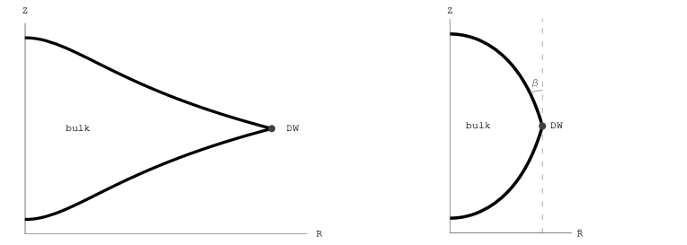
Figure 3: A Domain Wall (the thick dot) localized on the brane (the thick line). The full space consists of two copies of the bulk glued along the brane. The left panel is in the $R$ coordinate, which represents the Hubble radius of the 3D sections (here suppressed). The right panel is in the conformal coordinates, $Z$ and $\tilde{R}=\ell\arctan(R/\ell)$, in terms of which we can easily identify the deficit angle $\delta$. For positive brane tension $\tau$, the bulk corresponds to the interior, so $\delta=4\beta$. For $\tau<0$, the bulk is the exterior and $\delta=-4\beta$.

Now, let us see how this looks from the point of view of an observer living on the brane. Using (4.7), one easily obtains that the junction condition on the wall (4.12) translates into

$$K_{0}={\tau\over 6M^{3}}\tan\left({\sigma\over 4M^{3}}\right)~{},$$ (4.15)

where $K_{0}$ is as in (2.6). We see that the jump in the DW extrinsic curvature (i.e., its accelerated motion) is determined by the tensions of both the codimension 1 and the codimension 2 branes. This is expected since for $\tau=0$ the DW should not be accelerating, as any genuine codimension 2 brane.

Note as well that (4.15) together with (4.9) (with $\mu=0$) and (2.7) lead to the following relation for the Hubble rate with respect to the brane tensions and bulk cosmological constant,

$$H_{0}^{2}=\left({\tau\over 6M^{3}}\right)^{2}{1\over\cos^{2}\left({\sigma/4M^{3}}\right)}+{\Lambda_{5}\over 6M^{3}}~{}.$$ (4.16)

This can be viewed as the effective ‘Friedmann equation’ valid on the DW. As expected, for $\tau=0$ (an isolated codimension 2 brane), this trivially sets the Hubble rate equal to that of the bulk. However, in the presence of the codimension 1 brane, $H_{0}$ becomes sensitive to the energy density $\sigma$.

In summary, we have seen that the induced metric on the brane takes exactly the same form as in GR (a VIS spacetime or its generalizations with nonzero cosmological constant) except for the relation between $K_{0}$ (or $H_{0}$) and the tension $\sigma$. We leave for Sec. 4.4 the comparison between this result and the one obtained in the CFT description (3.12).

At this point, the first comment is that the linearized version of the exact result (4.15) correctly reproduces what one would find in the linear theory [20]. Indeed for $\tau>0$, the KK decomposition of the 5D graviton includes a zero mode coupled with an effective 4D Plank mass given by $\ell M^{3}$ together with a tower of massive gravitons. The latter do not couple to relativistic DWs [41], so the only effect comes from the zero mode, precisely matching (4.15) at linear level. For $\tau<0$ (and a single brane), the spectrum consists of a scalar zero mode (the radion), the massive KK gravitons and no graviton zero mode. Hence, the effect comes from the radion, which ‘explains’ the opposite sign in $K_{0}$.

Another important comment is that both $K_{0}$ and $H_{0}$ diverge when $\sigma$ approaches the critical value

$$\sigma_{c}^{(5)}=2\pi M^{3}~{},$$

that is, when the deficit angle saturates to $2\pi$. This is an unavoidable feature of accelerated codimension 2 branes and the reason can be traced back to the Gauss-Bonnet theorem applied to the (Euclideanized) space transverse to the DW. The theorem states that the Euler characteristic $\chi$ is given by

$$2\pi\chi=\int_{\cal M}\sqrt{g_{2}}d^{2}xR_{2}+\int_{\partial\cal M}\sqrt{g_{1}}dxK$$ (4.17)

where $R_{2}$ is the Ricci scalar of the space $\cal M$ transverse to the DW (with metric $g_{2}$) and $K$ is the extrinsic curvature at the boundary $\partial\cal M$. Since $\chi$ is a topological invariant, in particular it must be independent of the DW tension. Using the equations of motion, one finds a contribution from the DW tension (from the boundary integral). Away from the DW, the local curvatures $R_{2}$ and $K$ are constant and independent of $\sigma$. So, the only way that the integral is independent of $\sigma$ is that the integration volume changes. In our case, the topology of the transverse space is that of a disk, so $\chi=1$. When the DW tension approaches $2\pi M^{3}$, its contribution to the right hand side of (4.17) saturates to $2\pi$. Hence, the remaining ‘volume’ contribution has to vanish, which implies that $H_{0}^{-1}$ must vanish too.

This is of course related to the ‘pathology’ present for isolated codimension 2 branes. The opening angle of the conical transverse space is zero for critical tension, and the two transverse directions ‘collapse’ to a line. If one resolves the string thickness, however, one realizes that the transverse space is a cylinder with a radius of order of the thickness. Similarly, the divergence in $H_{0}$ and $K_{0}$ in the present case will be resolved by introducing the wall thickness. We defer this discussion to Section 4.3.

4.2 Beyond the horizon

Let us briefly comment on the properties of the bulk spacetime and especially on continuation through the horizon, with the purpose of showing explicitly that no pathologies, like Closed Timelike Curves (CTCs), are present. Specifically, we shall concentrate on the case $\kappa=1$.

The bulk of the above solution is locally AdS₅, which in the $R,\,Z$ coordinates takes the form

$$ds^{2}=\left(\kappa+\frac{R^{2}}{\ell^{2}}\right)dZ^{2}+\left(\kappa+\frac{R^{2}}{\ell^{2}}\right)^{-1}dR^{2}+R^{2}\;ds_{\kappa}^{2}\,.$$ (4.18)

These coordinates are convenient because the DW sits at a point in the $R,\,Z$ plane, and its Hubble radius is simply given by the value of the $R$ coordinate. While we will keep part of our discussion for generic $\kappa$, the case of most interest for us is going to be $\kappa=1$, when the DW inflates. In this case, the above coordinates do not cover all of AdS₅ because $R$ is a kind of Rindler coordinate. This can be readily seen from the form of the coordinate transformation that brings $R,\,Z$ to the Poincaré patch,

$$R = r\,e^{-y/\ell}$$ (4.19)

$$e^{2Z/\ell} = e^{2y/\ell}+(r/\ell)^{2}.$$ (4.20)

In terms of these, the metric is $ds^{2}=dy^{2}+e^{-2y\ell}(dr^{2}+r^{2}ds_{(\kappa=1)}^{2})$, so we identify $r$ as the usual Rindler coordinate of the 4D Minkowski sections (given by constant $y$ slices). Figure 4 depicts the relation between these coordinates. The constant $r$ lines are geodesics, while the constant $y$ are curves with uniform acceleration which precisely correspond to the location of a tuned RS brane (see below).

Figure 4: Contours of constant $y$ coordinate (solid line) and constant $r$ coordinate (dashed) in the $R,\,Z$ plane. $y$ is the proper coordinate in the Poincaré slicing of AdS₅ (see (4.19)). The dashed lines are (spacelike) geodesics, and measure the proper distance in the direction perpendicular to the brane. The solid lines correspond to the location of a ‘tuned’ RS brane, with a tension given by (4.8).

Now, let us discuss the continuation across the horizon. Starting from the metric (4.18) and writing the line element of the 3D sections as $-d\tau^{2}+\cosh^{2}\tau\,d\Omega^{2}$, where $d\Omega^{2}$ is the metric on the 2-sphere, the continuation across the Rindler horizon at $R=0$ is given by $R\to iT$ and $\tau\to\chi+i\pi/2$. Thus, the metric in the Milne region looks like

$$ds^{2}=\left(1-\frac{T^{2}}{\ell^{2}}\right)dZ^{2}-\left(1-\frac{T^{2}}{\ell^{2}}\right)^{-1}dT^{2}+T^{2}\;dH_{3}^{2}\,,$$ (4.21)

where $dH_{3}^{2}=d\chi^{2}+\sinh^{2}\chi d\Omega^{2}$ is the metric on the hyperbolic space. These coordinates are again singular at $T=\ell$. Hence, one has to do one more continuation, $Z\to\widetilde{T}+i\pi/2$, $T\to X$, and in this patch (with $X>\ell$) the metric takes the form

$$ds^{2}=-\left(\frac{X^{2}}{\ell^{2}}-1\right)d\widetilde{T}^{2}+\left(\frac{X^{2}}{\ell^{2}}-1\right)^{-1}dX^{2}+X^{2}\;dH_{3}^{2}\,.$$ (4.22)

Thus, $Z$ becomes a time coordinate when the radius of the 3D slices becomes larger than $\ell$.

In these coordinates, it is apparent how the BTZ black hole [57, 58] (and its higher dimensional generalization) arises. This is obtained simply by periodically identifying $Z$, which implies a periodic $\widetilde{T}$. In order not to have CTCs, one has to excise the region covered by $X\,,\widetilde{T}$. Then, the hypersurface $T=\ell$ plays the role of a singularity in the sense that geodesics terminate there.

Even though we did not make it manifest until now, we are assuming that $Z$ has a noncompact range (for $\kappa\neq-1$). At first, this seems to guarantee that the bulk is pure AdS₅ as opposed to a BTZ black hole. However, since we are doing a nontrivial identification by gluing two copies of the bulk by the brane location, we should make more explicit that this does not give rise to CTCs. In particular, this means that the brane trajectory must be such that its $Z$ coordinate goes to infinity when approaching $T=\ell$, otherwise the bulk contains CTCs with finite period. This turns out to be precisely what happens.

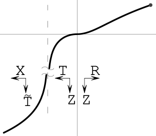
Figure 5: Form of the brane trajectory in the bulk. Only one ‘arm’ (one side of the DW) of the brane is shown. The continuous vertical line corresponds to the Rindler horizon. To the right of it, there is the Rindler region; to the left, there is the the Milne region,covered by the patches $T\,,Z$ and $X\,,\widetilde{T}$. The dashed axis corresponds to $T=X=\ell$, and is where $Z(t)$ and $\widetilde{T}(t)$ diverge.

For the tuned RS case, the induced metric on the brane takes the form of the VIS model described in Sec. 2. In the Rindler region, this is given by $R(\xi)=H_{0}^{-1}-|\xi|$. The continuation across the horizon gives a Milne universe, $-dt^{2}+t^{2}dH_{3}^{2}$ and the conformal diagram on the brane is the same as Fig 1. Hence, we can identify the trajectory in the $T\,,Z$ plane as $T(t)=t$ and $Z(t)$ as given by the continuation of (4.6). Similarly, in the region covered by the $X\,,\widetilde{T}$ coordinates, one has $X(t)=t$. One can easily see that $Z(t)=(1/2)\log(1-(t/\ell)^{2})$, so indeed $Z$ (and similarly $\widetilde{T}$) diverge for $T$ close to $\ell$. This is illustrated in Figure 5, where we show the form of the brane trajectory in a combined $(R\,,Z)$, $(T\,,Z)$ and $(X\,,\widetilde{T})$ plane.

In summary, there are no CTCs in the region covered by $X\,,\widetilde{T}$ so there is no need to excise this region. Ultimately, this means that the continuation of the brane geometry includes the whole Milne region and the conformal diagram is indeed given by Fig. 1.

4.3 Beyond the critical tension

In this Subsection, we shall see how the divergence of $H_{0}$ and $K_{0}$ when the DW tension reaches the critical value $2\pi M^{3}$ is resolved by introducing the DW thickness, $d$. As a byproduct, this allows us to find solutions for supermassive codimension 2 branes. In the next derivation, we will follow [41].

As it happens also in GR (see Section 2), once we introduce the DW thickness, one has to allow for a nonzero pressure in the direction orthogonal to the wall, $P$. Hence, the form of the stress tensor for the DW is as in (2.11). We do not need to specify the actual microscopic model for the domain wall, but we shall assume that its stress tensor is conserved on the brane, which leads to (2.12).

From (4.30) and (4.16), as soon as the DW tension $\sigma$ approaches $2\pi M^{3}$ both $H_{0}$ and $K_{0}$ grow very quickly beyond $1/\ell$. From the Gauss Codazzi equation (2.7), one also has that $H_{0}\sim|K_{0}|$ (for a moderate brane tension). In addition, we shall assume that the DW thickness $d$ is much smaller than $\ell$. In this case, there is a range of tensions for which

$$1/\ell\ll H_{0}\ll 1/d~{}.$$

In this regime, the DW is not yet in a phase of topological inflation, and we can still unambiguously speak of the DW. The interest of this range is that the DW experiences 5D gravity.

We can proceed essentially along the same steps as in the previous Subsection, but now including the pressure $P$

$$2\,M^{3}\;{\sqrt{f(R)-R^{\prime 2}}\over R}={\tau-P\over 3}~{},$$ (4.23)

For simplicity we will focus on the case $\tau=\tau_{RS}>0$ and we shall also assume that $P$ is everywhere less than $\tau$, so that the sign of the right hand side is positive.

Instead of computing explicitly the other component of the junction conditions, we can derive it as in Section 3, from (4.23). One obtains

$$-2\,M^{3}\left\{{R^{\prime\prime}\over\sqrt{f(R)-{R^{\prime}}^{2}}}+{1-R^{\prime 2}\over R\sqrt{f(R)-{R^{\prime}}^{2}}}\right\}=\rho+P.$$ (4.24)

As before, the idea is to integrate across the DW core this expression and obtain a junction condition on the DW. This time, we shall not only keep the $\delta$-function-like terms, since we want to keep track of the contribution from $P$. We must also take into account that the second term on the left hand side of (4.24) is of the same order as $P$. Using (4.23), we arrive at

$$-2\,M^{3}{R^{\prime\prime}\over\sqrt{f(R)-{R^{\prime}}^{2}}}=\rho+{1\over 3}P.$$ (4.25)

where we have ignored terms of order $P^{2}/\tau\ll P$.

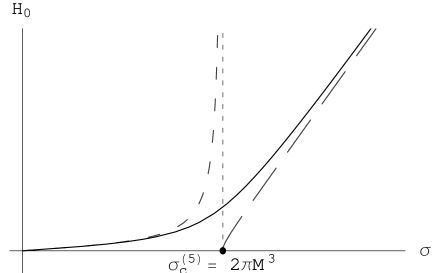
Figure 6: Relation between the DW Hubble rate $H_{0}$ and its tension $\sigma$ as given by (4.28) for $\ell/d=10$ (solid line). The singularity at $\sigma=\sigma_{c}^{(5)}$ in the thin wall limit (short dashed line) gets resolved. The long dashed line corresponds to a deficit angle equal to $2\pi$. As is apparent, even for supercritical tensions ($\sigma>\sigma_{c}^{(5)}$), the deficit angle is never saturated.

Integrating across the DW, one obtains the following matching condition

$$\frac{1}{2M^{3}}\left(\sigma+{1\over 3}\,d\,P_{0}\right)=-\,\Delta\;\arctan{R^{\prime}\over\sqrt{f(R)-{R^{\prime}}^{2}}}\simeq 2\,\arctan{\ell\over R_{0}}$$ (4.26)

where in the second equality we used that $H_{4}$ is much smaller than $K_{0},H_{0}$ and that in the core of the DW $R(\xi)$ stays close to its central value, $R(0)=1/H_{0}$. Also, we identified the DW tension as $\sigma=\int d\xi\rho$, and we defined the DW thickness by

$$d\equiv{1\over P_{0}}\int_{core}d\xi P~{}.$$

From (4.23), the pressure at the center of the core is given by

$${P_{0}\over 6M^{3}}={1-\sqrt{1+(H_{0}\ell)^{2}}\over\ell}~{}.$$ (4.27)

Putting these together, we find that $H_{0}$ now depends on $\sigma$ as

$$\arctan\left(H_{0}\ell\right)+{1\over 2}{d\over\ell}\left(\sqrt{1+(H_{0}\ell)^{2}}-1\right)={\sigma\over 4M^{3}}~{}.$$ (4.28)

We plot this relation in Fig. 6, where it is apparent that the singularity at $2\pi M^{3}$ in (4.16) and (4.15) is resolved. Note that even though we can have $\sigma>2\pi M^{3}$, the deficit angle (which is given by the first term in the left hand side of (4.28)) never exceeds $2\pi$.

As expected, the contribution from $P$ in (4.28) vanishes for $d\to 0$. However, this term allows us to have supercritical solutions. Indeed, for $\sigma\gg 2\pi M^{3}$ one has $H_{0}\ell\gg 1$ and (4.28) approximates to

$$H_{0}\simeq{\sigma-2\pi M^{3}\over 2dM^{3}}~{}.$$ (4.29)

This is similar to a usual DW with an effective 4D Planck mass of order $dM^{3}$. So, in this regime, the gravitational effect of the DW is enhanced by a factor $\ell/d$. The change of behaviour always takes place for $\sigma$ close to $2\pi M^{3}$ (and consequently $H_{0}$ close to $1/\ell$).

This new regime should be identified as the five dimensional behaviour not just because $H_{0}\gg 1/\ell$, but also because this is how a (supermassive) codimension 2 branes behave [41]. Indeed, for subcritical tensions, codimension 2 branes do not inflate, rather they only produce a deficit angle given by $\sigma/M^{3}$. For critical tension, the transverse space becomes a cylinder of radius of order $d$. Hence, the space is effectively compactified to one dimension less, with an effective Planck mass of order $dM^{3}$. For supercritical tension, there are no regular static solutions [59, 60, 61], but inflating ones may exist [62, 63]. This is perfectly compatible with the fact that the transverse space has been compactified, so the brane effectively behaves as a codimension 1 object from the lower dimensional point of view. Moreover, the brane ‘spends’ part of its tension ($2\pi M^{3}$ to be precise) compactifying, and the remainder in how much it inflates. Hence, the gravitational effect of a supermassive codimension 2 is to inflate precisely according to (4.29), and we conclude that the DW is exhibiting a 5D behaviour as opposed to a 4D one (which would give $H_{0}\simeq\sigma/4M_{\rm Pl}^{2}$).

We should add that once the DW experiences this 5D gravity, $\sigma$ does not need to be much larger than $2\pi M^{3}$ before topological inflation sets in. Indeed, for $\sigma\simeq 2(\pi+1)M^{3}$ one already has $H_{0}\simeq 1/d$ in (4.29).

This behaviour has simple interpretation in terms of the microscopic model for the topological defect. We have in mind a scalar field model with a quartic potential, but this discussion should be rather generic. As it turns out, both for Domain Walls [43] an cosmic strings [62, 63], the topological inflation starts when the vev of the scalar field $\langle\phi\rangle$ (the location of the degenerate minimum) is of order of the Planck mass. What happens with the localized DWs is that they can be viewed both as a codimension 1 and a codimension 2 objects, and the associated Planck scales for each behaviour are different. As a result, from the 4D point of view, topological inflation is ‘prematurely’ reached for $\langle\phi\rangle$ of order $M$, rather than the naively expected $M_{\rm Pl}$.

4.4 Comparison with the CFT

Let us now see how the results of the previous subsection are in agreement with the dressed DW picture of Section 3. Starting by the most general case, when the brane tension is not tuned to $\tau_{RS}$, we set $\tau=\tau_{RS}+\delta\tau$ with $\tau_{RS}$ defined in (4.8). We can rewrite (4.15) as

$${1\over\ell}\arctan\left({K_{0}\ell\over 1+\delta\tau/\tau_{RS}}\right)={\sigma\over 4M_{\rm Pl}^{2}}~{}.$$ (4.30)

where we used $M_{\rm Pl}^{2}=\ell M^{3}$. Expanding to the leading order correction, one obtains

$$K_{0}\left(1-{\delta\tau\over\tau_{RS}}-{1\over 3}(K_{0}\ell)^{2}+\dots\right)={\sigma\over 4M_{\rm Pl}^{2}}~{}.$$ (4.31)

From (4.9) (with $\mu=0$), the curvature scale on the brane away from the DW is $H_{4}^{2}=\Lambda_{4}^{\rm eff}/3M_{\rm Pl}^{2}$, with $\Lambda_{4}^{\rm eff}$ given in (4.10). To leading order in $\delta\tau$, one can rewrite this as $\delta\tau/\tau_{RS}=(H_{4}\ell)^{2}/2$. Using this and the Gauss Codazzi equation (2.7), we find

$$K_{0}\left(1-{1\over 2}(H_{0}\ell)^{2}+{1\over 6}(K_{0}\ell)^{2}+\dots\right)={\sigma\over 4M_{\rm Pl}^{2}}~{}.$$ (4.32)

This is exactly the same as (3.11) once we use (3.13). For the tuned RS case, $\delta\tau=0$, and it is straightforward that (4.31) leads to (3.12).

Hence, we explicitly see that the ‘cutoff’ AdS/CFT correspondence works at the level of matching the correct numerical factors. As mentioned before, this is due to the fact that in the CFT side the only effects are due to the anomaly, which guarantees that the results at small ’t Hooft coupling (which is what we compute in the 4D side) and at strong coupling (which is what the gravity side gives) must coincide. Note that this is not true for the case that we left out of our analysis, when the DW worldvolume is AdS₃, because the state dependent contribution from the CFT (3.3) may be nontrivial.

As the reader might have noticed already, the results in both sides of the correspondence (3.12) and (4.30) are exact, and yet we find agreement in the first two terms of the expansion in powers of $K_{0},H_{0}$ (see (4.32)) only. One can ask what these corrections correspond to in the CFT. These terms are of the form $K_{0}(N^{2}K_{0}^{2}/M_{\rm Pl}^{2})^{n}$ for $n=1,2\dots$ However, the loop corrections can be arranged as a $1/N^{2}$ expansion and the leading order is proportional to $N^{2}$. So, these corrections do not come from higher (CFT or graviton) loops. Rather, these are terms that vanish when the cutoff is removed, as it is manifest since they are suppressed by the cutoff, $1/\ell$. Hence from the point of view of the 4D effective theory they are un-calculable and were implicitly set to zero in Section 3. In the particular UV completion of the 4D theory provided by the RS setup, instead, they are organized according to the expansion of (4.30).

Still, the fact that the 4D analysis breaks down for $\sigma>\sigma_{c}^{(4)}$ (with $\sigma_{c}^{(4)}$ given in (3.14)) signals that the UV completion should change regime at around that scale. As we have seen in Section 4.3, this is indeed the case in the RS setup as the DW starts behaving in a 5D fashion for tensions around $\sigma_{c}^{(5)}$, which is parameterically close to $\sigma_{c}^{(4)}$.

5 Conclusions

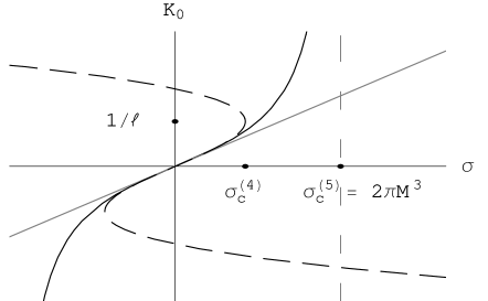
Figure 7: This plot summarizes the comparison between the two sides of the correspondence. The solid line is the RS result (4.15), the dashed line is the outcome from the CFT side (3.12), for vanishing cosmological constant. We also include for reference the GR result (solid gray line). For small enough tensions, the curves from the RS and the CFT results agree beyond the GR result.

The cutoff version of the AdS/CFT correspondence is a powerful tool to learn how a (strongly coupled) CFT behaves in the presence of gravity. In this respect, one of the most relevant problems that are still being debated is how the black hole evaporation takes place in this setup and, correspondingly, whether static solutions for black holes localized on the brane exist [22, 23, 28, 29]. In this paper we have studied a much simpler case, namely how the CFT responds to the gravitational field produced by a Domain Wall (DW). This is a physical implementation of a moving mirror so, generically, one may expect the presence of particle creation. Hence, this case represents a ‘toy’ example where phenomena similar to Hawking radiation may arise.

We have allowed for an arbitrary cosmological constant $\Lambda_{4}$, and we have restricted ourselves to the case when the DW worldvolume is maximally symmetric. For $\Lambda_{4}\geq 0$, the DW always develops a horizon while for $\Lambda_{4}<0$ it only does so if its tension is large enough. Whenever the horizon is present, the conformality of the field theory is enough to see that there is no particle creation. Given that this follows from very general assumptions concerning the symmetry of the configuration and the regularity of the vacuum, this result should hold to all orders in the loop expansion. The computation in the 5D dual (which is valid at large ’t Hooft coupling) confirms that this is the case. The absence of particle production can also be understood from the classic results for moving mirrors. When the DW is maximally symmetric, its motion has a constant acceleration, it is well knonw that in this case there is no radiation into conformal fields.

However, the CFT still leads to some effect because the trace anomaly plays a nontrivial role. This is non-zero on the DW worldvolume and effectively renormalizes the tension. Hence, there is a correction to the gravitational field produced by the DW. We computed it explicitly both in the CFT (at 1-loop) and in the Randall-Sundrum sides of the correspondence, and find a precise agreement to the numerical factors. The reason for the numerical match is that the correction is entirely due to the conformal anomaly, which has no contributions beyond 1-loop in an ${\cal N}=4$ SYM.

In the RS side, the computation involves finding solutions for a DW localized on the brane, that is for a codimension 2 brane (the DW) embedded on the RS brane. Because of the localization, the codimension 2 brane behaves very differently from how it would in isolation. The RS brane ‘pulls’ the codimension 2 brane which, as a result, moves with uniform acceleration. Hence, it effectively generates a repulsive gravitational field and, from the point of view of the observers on the brane, looks like a Domain Wall.

As already emphasized, the amount of symmetries of the case studied here precludes the DW from radiating CFT quanta. Hence, there is little that we can add to the black hole debate. However, our analysis can be extended in several directions (e.g., assuming less worldvolume symmetry, a different equation of state on the wall or including other fields in the bulk), some of which may lead to particle creation and still be tractable. One promising case is offered by DWs in AdS₄ when the tension is low enough so that the worldvolume is AdS₃. In this case, the wall is still in an accelerated motion but there is no horizon, so there is no obstruction for particle production. We shall report on this case soon.

Appendix A 1-Loop correction to the graviton propagator

In Section 3, we described how to obtain the correction the gravitational field of a DW generated by the CFT. Using the symmetries of the problem and the properties of the CFT we concluded that there would be no correction were it not for the trace anomaly. We shall now show this more directly, by computing explicitly the first loop correction to the graviton propagator due to the CFT, and the linearized field that this gives entails. As we shall see, the 1-loop contribution to the metric perturbation is pure gauge, so gravitational field is not affected by the CFT radiative correction. This derivation does not capture the anomalous term because it is expanded around flat space, where the anomaly is zero. In this appendix, we shall follow Ref. [21].

The metric fluctuation around flat space $h_{\mu\nu}=g_{\mu\nu}-\eta_{\mu\nu}$ can be expressed in momentum space as

$$\hat{h}_{\mu\nu} = -16\pi G_{\mathrm{N}}\,\Delta_{(4)}(p)\left[\hat{T}^{\,\mathrm{DW}}_{\mu\nu}-\frac{1}{2}\eta_{\mu\nu}\hat{T}^{\,\mathrm{DW}}\right]+$$ (A.1)

$$-16\pi\,G_{\mathrm{N}}\left[2\Pi_{2}(p)\hat{T}^{\,\mathrm{DW}}_{\mu\nu}+\Pi_{1}(p)\eta_{\mu\nu}\hat{T}^{\,\mathrm{DW}}\right]\,,$$

where the first term $\Delta_{(4)}$ is the tree level propagator in four dimensions, while the second is the graviton self-energy at first loop, and only conformal fields are running in the loop. The form factors $\Pi_{i}$ are dictated by symmetries of CFT, and have the following explicit form

$$\Pi_{i}=32\pi G_{\mathrm{N}}\,\left[a_{i}\,\ln\frac{p^{2}}{\mu^{2}}+b_{i}\right]\quad,i=1,2\\$$ (A.2)

where $b_{i}$ are some irrelevant constants and

$$a_{i}^{(1)}=4a_{i}^{(1/2)}=12a_{i}^{(0)}=\frac{1}{120\,(4\pi)^{2}}(-2,3)\,,$$ (A.3)

with the superscript on the parameter $a_{i}^{(s)}$ referring to vectors $s=1$, fermions $s=1/2$, and scalars $s=0$. The stress-energy tensor $\hat{T}^{\,\mathrm{DW}}_{\mu\nu}$ is

$$T_{\mu\nu}^{\,\mathrm{DW}}=-\left(\begin{array}[]{cc}\eta_{\alpha\beta}&0\\ 0&0\end{array}\right)\sigma\,\delta(z)\quad\Rightarrow\quad\hat{T}_{\mu\nu}^{\,\mathrm{DW}}=-\left(\begin{array}[]{cc}\eta_{\alpha\beta}&0\\ 0&0\end{array}\right)\sigma\,\delta^{\parallel}(p)\,,$$

where $\parallel$ represents the directions along the DW, and $\alpha\beta\dots$ are indices along these directions. With this, the 1-loop contribution becomes, upon Fourier-transforming back to space coordinates,

$$h_{\alpha\beta}^{(1-loop)} = \kappa_{1}\frac{G_{\mathrm{N}}^{2}\sigma}{z}\eta_{\alpha\beta}\,,$$ (A.4)

$$h_{zz}^{(1-loop)} = -\kappa_{2}\frac{G_{\mathrm{N}}^{2}\sigma}{z}\,.$$ (A.5)

The parameters $\kappa_{i}$ are found to be $\kappa_{1}=0$ as the contributions from $\Pi_{1}$ and $\Pi_{2}$ cancel, and

$$\kappa_{2}=\frac{a}{120\pi}=-\frac{N^{2}}{4\pi}\,,$$ (A.6)

where $a=\sum_{s}N^{(s)}a_{1}^{(s)}=-5N^{2}$ for the field content of $\mathcal{N}=4$ Super Yang-Mills theory with gauge group $SU(N)$. Hence, the correction to the linearized metric due to the 1-loop diagrams of the CFT has $h_{\alpha\beta}^{(1-loop)}=0$ and

$$h_{zz}^{(1-loop)}=\frac{G_{\mathrm{N}}^{2}N^{2}}{4\pi\,z}\sigma~{}.$$

This is clearly of pure gauge form, so we conclude that the CFT does not correct the field created by a DW at 1-loop. Let us insist that this is no longer true once the trace anomaly is properly accounted for, which is possible only if we make an ansatz where the DW is already inflating.

Let us end by noting that the result of this Appendix is expected to hold at all orders in the loop expansion. This can be proven in an elegant way by performing a Källen-Lehmann decomposition of the graviton propagator. This is going to have a pole at $p^{2}=0$ and a branch cut, which is dual to the massless graviton and the continuum of massive Kaluza Klein modes that appear in RS. Given that the massive gravitons couple to matter through the combination $h_{\mu\nu}\sim\Delta(p)[T_{\mu\nu}-(T/3)\eta_{\mu\nu}]$, for relativistic Domain Walls this always leads to a pure gauge form. Hence, massive gravitons do not couple to the walls at least to linear order, and irrespective of the actual form of the form factor $\Delta$ or $\Pi_{i}$, the CFT radiative corrections at any loop order should vanish.

References

- [1] J. M. Maldacena, “The large N limit of superconformal field theories and supergravity,” Adv. Theor. Math. Phys. 2 (1998) 231–252, hep-th/9711200.
- [2] E. Witten, “Anti-de Sitter space and holography,” Adv. Theor. Math. Phys. 2 (1998) 253–291, hep-th/9802150.
- [3] S. S. Gubser, I. R. Klebanov, and A. M. Polyakov, “Gauge theory correlators from non-critical string theory,” Phys. Lett. B428 (1998) 105–114, hep-th/9802109.
- [4] O. Aharony, S. S. Gubser, J. M. Maldacena, H. Ooguri, and Y. Oz, “Large N field theories, string theory and gravity,” Phys. Rept. 323 (2000) 183–386, hep-th/9905111.
- [5] H. L. Verlinde, “Holography and compactification,” Nucl. Phys. B580 (2000) 264–274, hep-th/9906182.
- [6] S. S. Gubser, “AdS/CFT and gravity,” Phys. Rev. D63 (2001) 084017, hep-th/9912001.
- [7] N. Arkani-Hamed, M. Porrati, and L. Randall, “Holography and phenomenology,” JHEP 08 (2001) 017, hep-th/0012148.
- [8] L. Randall and R. Sundrum, “An alternative to compactification,” Phys. Rev. Lett. 83 (1999) 4690–4693, hep-th/9906064.
- [9] S. W. Hawking, T. Hertog, and H. S. Reall, “Trace anomaly driven inflation,” Phys. Rev. D63 (2001) 083504, hep-th/0010232.
- [10] E. P. Verlinde, “On the holographic principle in a radiation dominated universe,” hep-th/0008140.
- [11] I. Savonije and E. P. Verlinde, “CFT and entropy on the brane,” Phys. Lett. B507 (2001) 305–311, hep-th/0102042.
- [12] S. Nojiri and S. D. Odintsov, “AdS/CFT correspondence, conformal anomaly and quantum corrected entropy bounds,” Int. J. Mod. Phys. A16 (2001) 3273–3290, hep-th/0011115.
- [13] T. Shiromizu and D. Ida, “Anti-de Sitter no hair, AdS/CFT and the brane-world,” Phys. Rev. D64 (2001) 044015, hep-th/0102035.
- [14] T. Shiromizu, T. Torii, and D. Ida, “Brane-world and holography,” JHEP 03 (2002) 007, hep-th/0105256.
- [15] T. Tanaka, “AdS/CFT correspondence in a Friedmann-Lemaitre-Robertson- Walker brane,” gr-qc/0402068.
- [16] A. Chamblin, S. W. Hawking, and H. S. Reall, “Brane-world black holes,” Phys. Rev. D61 (2000) 065007, hep-th/9909205.
- [17] J. Garriga and M. Sasaki, “Brane-world creation and black holes,” Phys. Rev. D62 (2000) 043523, hep-th/9912118.
- [18] R. Emparan, G. T. Horowitz, and R. C. Myers, “Exact description of black holes on branes,” JHEP 01 (2000) 007, hep-th/9911043.
- [19] R. Emparan, G. T. Horowitz, and R. C. Myers, “Exact description of black holes on branes. ii: Comparison with BTZ black holes and black strings,” JHEP 01 (2000) 021, hep-th/9912135.
- [20] J. Garriga and T. Tanaka, “Gravity in the brane-world,” Phys. Rev. Lett. 84 (2000) 2778–2781, hep-th/9911055.
- [21] M. J. Duff and J. T. Liu, “Complementarity of the Maldacena and Randall-Sundrum pictures,” Class. Quant. Grav. 18 (2001) 3207–3214, hep-th/0003237.
- [22] T. Tanaka, “Classical black hole evaporation in Randall-Sundrum infinite braneworld,” Prog. Theor. Phys. Suppl. 148 (2003) 307–316, gr-qc/0203082.
- [23] R. Emparan, A. Fabbri, and N. Kaloper, “Quantum black holes as holograms in AdS braneworlds,” JHEP 08 (2002) 043, hep-th/0206155.
- [24] R. Emparan, J. Garcia-Bellido, and N. Kaloper, “Black hole astrophysics in AdS braneworlds,” JHEP 01 (2003) 079, hep-th/0212132.
- [25] M. Bruni, C. Germani, and R. Maartens, “Gravitational collapse on the brane,” Phys. Rev. Lett. 87 (2001) 231302, gr-qc/0108013.
- [26] P. R. Anderson, R. Balbinot, and A. Fabbri, “Cutoff AdS/CFT duality and the quest for braneworld black holes,” Phys. Rev. Lett. 94 (2005) 061301, hep-th/0410034.
- [27] R. Casadio and C. Germani, “Gravitational collapse and black hole evolution: Do holographic black holes eventually ’anti-evaporate’?,” Prog. Theor. Phys. 114 (2005) 23–56, hep-th/0407191.
- [28] A. L. Fitzpatrick, L. Randall, and T. Wiseman, “On the existence and dynamics of braneworld black holes,” JHEP 11 (2006) 033, hep-th/0608208.
- [29] A. Fabbri and G. P. Procopio, “Quantum effects in black holes from the Schwarzschild black string?,” arXiv:0704.3728 [hep-th].
- [30] A. Fabbri, S. Farese, J. Navarro-Salas, G. J. Olmo, and H. Sanchis-Alepuz, “Semiclassical zero-temperature corrections to Schwarzschild spacetime and holography,” Phys. Rev. D73 (2006) 104023, hep-th/0512167.
- [31] T. Tanaka, “Implication of classical black hole evaporation conjecture to floating black holes,” arXiv:0709.3674 [gr-qc].
- [32] N. D. Birrell and P. C. W. Davies, “Quantum fields in curved space,”. Cambridge, Uk: Univ. Pr. ( 1982) 340p.
- [33] P. C. W. Davies and S. A. Fulling, “Radiation from moving mirrors and from black holes,” Proc. Roy. Soc. Lond. A356 (1977) 237.
- [34] P. C. W. Davies and S. A. Fulling, “Radiation from a moving mirror in two-dimensional space- time conformal anomaly,” Proc. Roy. Soc. Lond. A348 (1976) 393–414.
- [35] P. Candelas and D. Deutsch, “On the vacuum stress induced by uniform acceleration or supporting the ether,” Proc. Roy. Soc. Lond. 354 (1977) 79.
- [36] V. P. Frolov and E. M. Serebryanyi, “Quantum effects in systems with accelerated mirrors.,” J. Phys. A12 (1979) 2415–2428.
- [37] R. D. Carlitz and R. S. Willey, “Reflections on moving mirrors,” Phys. Rev. D36 (1987) 2327.
- [38] R. D. Carlitz and R. S. Willey, “The lifetime of a black hole,” Phys. Rev. D36 (1987) 2336.
- [39] A. Vilenkin, “Gravitational field of vacuum domain walls,” Phys. Lett. B133 (1983) 177–179.
- [40] J. Ipser and P. Sikivie, “The gravitationally repulsive domain wall,” Phys. Rev. D30 (1984) 712.
- [41] G. Dvali, G. Gabadadze, O. Pujolas, and R. Rahman, “Domain walls as probes of gravity,” hep-th/0612016.
- [42] G. W. Gibbons, “Global structure of supergravity domain wall space- times,” Nucl. Phys. B394 (1993) 3–20.
- [43] A. Vilenkin, “Topological inflation,” Phys. Rev. Lett. 72 (1994) 3137–3140, hep-th/9402085.
- [44] L. M. Widrow, “General relativistic domain walls,” Phys. Rev. D39 (1989) 3571.
- [45] E. Witten, “Instability of the Kaluza-Klein vacuum,” Nucl. Phys. B195 (1982) 481.
- [46] O. Aharony, M. Fabinger, G. T. Horowitz, and E. Silverstein, “Clean time-dependent string backgrounds from bubble baths,” JHEP 07 (2002) 007, hep-th/0204158.
- [47] D. Birmingham and M. Rinaldi, “Bubbles in Anti-de Sitter space,” Phys. Lett. B544 (2002) 316–320, hep-th/0205246.
- [48] V. Balasubramanian and S. F. Ross, “The dual of nothing,” Phys. Rev. D66 (2002) 086002, hep-th/0205290.
- [49] V. Balasubramanian, K. Larjo, and J. Simon, “Much ado about nothing,” Class. Quant. Grav. 22 (2005) 4149–4170, hep-th/0502111.
- [50] O. Pujolas and T. Tanaka, “Massless scalar fields and infrared divergences in the inflationary brane world,” JCAP 0412 (2004) 009, gr-qc/0407085.
- [51] O. Pujolas and M. Sasaki, “Vacuum destabilization from Kaluza-Klein modes in an inflating brane,” JCAP 0509 (2005) 002, hep-th/0507239.
- [52] X. Montes, “Renormalized stress tensor in one-bubble spacetimes,” Int. J. Theor. Phys. 38 (1999) 3091–3109, gr-qc/9904022.
- [53] A. A. Starobinsky, “A new type of isotropic cosmological models without singularity,” Phys. Lett. B91 (1980) 99–102.
- [54] A. Vilenkin, “Classical and quantum cosmology of the Starobinsky inflationary model,” Phys. Rev. D32 (1985) 2511.
- [55] G. Dvali, “Black holes and large N species solution to the hierarchy problem,” arXiv:0706.2050 [hep-th].
- [56] R. Gregory and A. Padilla, “Nested braneworlds and strong brane gravity,” Phys. Rev. D65 (2002) 084013, hep-th/0104262.
- [57] M. Banados, C. Teitelboim, and J. Zanelli, “The black hole in three-dimensional space-time,” Phys. Rev. Lett. 69 (1992) 1849–1851, hep-th/9204099.
- [58] M. Banados, M. Henneaux, C. Teitelboim, and J. Zanelli, “Geometry of the (2+1) black hole,” Phys. Rev. D48 (1993) 1506–1525, gr-qc/9302012.
- [59] I. Gott, J. Richard, “Gravitational lensing effects of vacuum strings: Exact solutions,” Astrophys. J. 288 (1985) 422–427.
- [60] M. E. Ortiz, “A new look at supermassive cosmic strings,” Phys. Rev. D43 (1991) 2521–2526.
- [61] P. Laguna and D. Garfinkle, “Space-time of supermassive U(1) gauge cosmic strings,” Phys. Rev. D40 (1989) 1011–1016.
- [62] A. A. de Laix, M. Trodden, and T. Vachaspati, “Topological inflation with multiple winding,” Phys. Rev. D57 (1998) 7186–7191, gr-qc/9801016.
- [63] I. Cho, “Inflation and nonsingular spacetimes of cosmic strings,” Phys. Rev. D58 (1998) 103509, gr-qc/9804086.