Evidence for Tadpole Cancellation in the Topological String

arXiv:0712.2775

December 2007

1 Introduction

In this paper we continue, and in a sense complete, the program of extending the BCOV [1, 2] computation of perturbative topological string amplitudes on compact Calabi-Yau manifolds to the open string sector. The main novelty is the realization that the inclusion of non-orientable worldsheets appears unavoidable for a satisfactory physical interpretation of the open topological string (at least beyond tree-level), on compact Calabi-Yau manifolds.

There is of course no consistency condition that would be more familiar to string theorists than the cancellation of anomalies in the ten-dimensional superstring [3]. As is well-known [4], the potential anomalies can be seen to originate from tadpoles of unphysical, BRST trivial states from the Ramond-Ramond sector. These anomalies and the associated infinities can only be removed by ensuring that the Ramond-Ramond tadpoles are canceled at tree-level. This is in distinction to NS-NS sector tadpoles, which can in principle be adjusted by a Fischler-Susskind mechanism. The general principle, outlined in [5], is that anomalies in string theory can always be thought of as arising from boundary (surface) terms on the moduli space in the verification of decoupling of BRST trivial states from loop amplitude computations.

Similar comments apply to modern constructions using the type I/II superstring, whenever the space transverse to the D-branes and orientifold planes is compact [6]. In supersymmetric situations, orientifold planes are the only known sinks of Ramond-Ramond charge, which the D-brane configuration has to be adjusted to match. In this way, tadpole/anomaly cancellation remains at the center of the idea that a consistent coupling to a fundamental theory of quantum gravity restricts the possible gauge and matter content to a finite set of possibilities, uniquely realized in string theory.

Given its central importance in the superstring, it has always seemed natural to ask whether tadpole cancellation has an analogue in the topological phase of string theory [7]. The topological string otherwise shares many features with its more physical counterparts and is moreover related to them by many more or less direct links. That tadpole cancellation indeed plays a role in the topological string was anticipated in the previous paper [8], in the sense that loop amplitudes involving open strings are only well-defined in sectors in which the total topological D-brane charge vanishes. In this paper, we will find further corroboration of this statement. Moreover, we will analyze the possibility of canceling the tadpoles using orientifolds, which was also mentioned in [8]. The precise statement and implications will be clear by the end of the introduction.

At this point, we do not have a microscopic understanding of the tadpole cancellation condition, although we can give a rough sketch of its possible worldsheet origin. Recall that the gauge algebra of the topological string coincides with that of the bosonic string, and originates from the topological twist of an underlying unitary ${\cal N}=2$ superconformal field theory. The identification between BRST operators, anti-ghosts, and ghost number current on the one hand and the ${\cal N}=2$ superconformal generators on the other hand is as follows:

$$\begin{array}[]{ccc}(Q,\bar{Q})&\leftrightarrow&(G^{+},\bar{G}^{+})\\ (b_{0},\bar{b}_{0})&\leftrightarrow&(G^{-},\bar{G}^{-})\\ (bc,\bar{b}\bar{c})&\leftrightarrow&(J,\bar{J})\end{array}$$ (1.1)

More precisely, the identification we have given in (1.1) is usually labeled as “type B”, the associated topological string called the B-model. The A-model arises from the identification in which $\bar{G}^{+}$ and $\bar{G}^{-}$ are exchanged on the RHS and $\bar{J}\to-\bar{J}$. A peculiarity of the topological string that distinguishes it from more conventional bosonic string backgrounds, is the absence of a ghost field as adjoint of the anti-ghost. In the underlying ${\cal N}=2$ SCFT, worldsheet CPT conjugation relates $(G^{+},\bar{G}^{+})$ with $(G^{-},\bar{G}^{-})$. Using the dictionary (1.1), this leads to the statement that the anti-ghost (i.e., $(b_{0},\bar{b}_{0})$) cohomology is isomorphic to the BRST cohomology, and in particular non-trivial, in clear distinction to the 26-dimensional bosonic string. The model obtained from the identification $(Q,\bar{Q})\leftrightarrow(G^{-},\bar{G}^{-})$ is referred to as the anti-topological B-model.

It was realized by Bershadsky, Cecotti, Ooguri and Vafa [1, 2] that the non-trivial states of the anti-ghost cohomology do not decouple from the topological amplitudes. The failure originates from the boundary of moduli space and can be viewed as an anomaly in accord with the above mentioned general principle. In distinction to gauge anomalies in the superstring, this so-called holomorphic anomaly is not fatal for the model. Instead, it can be expressed as a recursive derivative constraint on the perturbative topological string amplitudes. In this way, it has become a central ingredient in the successful computation of topological string amplitudes in various situations over the years, as well as having various other interesting connections.

The BCOV holomorphic anomaly equation was recently extended to the open string in [8]. Similar equations, which can in fact be understood as a special case of the equations of [8], were obtained in [9, 10] from the study of matrix models. Earlier work on the holomorphic anomaly in the open string appears in [2, 11], more recent work includes [12, 13, 14, 15]. For the wavefunction interpretation of the open topological string along the lines of [16], see [17, 18, 19].

Another feature of the origin of the topological string in twisted ${\cal N}=2$ SCFTs is that the mixed BRST-anti-ghost cohomology is non-trivial. Indeed, changing the identification of (1.1) to $(Q,\bar{Q})\leftrightarrow(G^{+},\bar{G}^{-})$ simply leads to the A-model on the same Calabi-Yau manifold, which is generically non-trivial. It was shown in [2] that the A-model deformations decouple from the topological B-model amplitudes. This argument was tailored to closed string topological amplitudes, and must be reexamined in the presence of boundaries, for the following reason.

It is a fundamental observation [20] that the topological charges of D-branes from the B-model are carried by the A-model, and vice-versa. For instance, A-branes on a Calabi-Yau manifold are supported on Lagrangian submanifolds, and the associated middle-dimensional cycles are naturally observables in the topological B-model. By combining this observation with the statements from the previous paragraphs, it is natural to view the $(G^{+},\bar{G}^{-})$-cohomology as the topological string analogue of the compact RR gauge potentials in the superstring. And by further analogy, it is natural to expect that the decoupling of A- and B-model, which is presumably violated in the presence of D-branes, will in fact be restored precisely when the tadpoles are canceled, i.e., the total topological D-brane charge vanishes.

The evidence for tadpole cancellation that we will present in this paper involves the relation of the topological string to BPS state counting in M-theory [21, 22]. In more detail, we will proceed as follows. We will begin in section 2 with a brief review of orientifold backgrounds of topological string. This will be useful later on when we cancel the tadpoles using orientifolds, and will also establish some notation. We then turn to some explicit A-model calculations in section 3. The examples we study include the quintic in ${\mathbb{P}}^{4}$, the bicubic in ${\mathbb{P}}^{5}$, and the total space of ${\cal O}_{{\mathbb{P}}^{2}}(-3)$, where in each case the Lagrangian brane is the real locus (with respect to the natural complex conjugation on projective space). The method we will use is essentially Kontsevich’s localization calculus on the space of stable maps [23], appropriately adapted to open and unoriented string computations. This is similar to refs. [24, 25, 26, 27, 28, 29, 30], with certain new ingredients, and will lead to a computation of higher genus open/unoriented Gromov-Witten invariants on the three spaces mentioned above (the method can certainly be extended to many other examples). Strictly speaking, the requisite definitions in Gromov-Witten theory have not been given yet, so our results depend on certain assumptions during the localization procedure, and our confidence that these assumptions are correct depends on the overall consistency of the results, and on the agreement with the B-model.

The surprise occurs when we plug these higher-genus open Gromov-Witten invariants into the general multi-cover formula of [21, 22, 31]. Namely, when these formulas are applied naively, the resulting expansion coefficients are not integer, and hence cannot be interpreted in terms of the spectrum of BPS states of an M-theory compactification on the Calabi-Yau manifold. It turns out, however, that when we add the contributions from orientable and non-orientable worldsheets, at fixed order in string perturbation theory, and then judiciously apply the multi-cover formulas of [22, 31], then the resulting expansion coefficients are integer. The relative coefficient between orientable and non-orientable worldsheets is consistent with the identification of the D-brane charge of the orientifold plane in [32]. The BPS interpretation of topological string amplitudes on orientifolds was also studied in [33, 34] for freely acting orientifolds on non-compact manifolds, where the effects that we discuss here play no role.

Thus girt with some explicit A-model results as benchmark, we turn in section 4 to formal developments to reproduce and complete these computations in the B-model. In particular, we write down an extension of the holomorphic anomaly equation of [2, 8] to unoriented strings. We will also see that the holomorphic anomaly equation for the total topological string amplitudes, cf., eq. (2.11), simplifies, and is in fact very simply related to the extended holomorphic anomaly equation of [8].

In section 5, we will then solve these generalized holomorphic anomaly equations for the examples at hand. We will be able to fix the holomorphic ambiguities to match the A-model computations of section 3, thus completing the mirror symmetric picture. The ability to fix the holomorphic ambiguity is a non-trivial check if we have more A-model data than free parameters in the B-model. In fact, there is a certain class of worldsheets for which we can extract the general form of the holomorphic ambiguity to all orders, in a way reminiscent of the results in [35, 10, 36].

The results for the holomorphic ambiguities in section 5 differ from those in [8], which were obtained by a more naive application of the multi-cover formulas, and imposing integrality and low-degree vanishing of the putative BPS invariants.

Finally, we summarize and discuss other open issues in section 6.

2 Orientifold of Topological String

An orientifold background in string theory is the result of gauging [37, 38, 39, 40] a closed string background, say $M$, by the combined action of worldsheet parity $\Omega$ with an involutive target space symmetry $\sigma:M\to M$. We will denote the combined symmetry by $P$,

$$P=\sigma\circ\Omega$$ (2.1)

as well as various other incarnations of $P$ such as the corresponding operator acting on the space of string states. As mentioned in the introduction, simply modding out by $P$ will in general lead to inconsistencies due to massless tadpoles and anomalies. Tadpole cancellation requires the inclusion of some D-brane configuration in the background, with a certain fixed total charge determined by the parity $P$.

One can equivalently think of an orientifold as a more conventional theory of strings propagating on the space $M/\sigma$, together with dynamics of unoriented strings localized around the geometrical fixed point loci of $\sigma$ (orientifold planes), as well as open string dynamics localized around the locations of the D-branes.

2.1 Orientifolds of Calabi-Yau manifolds

Compactifying the type IIA or type IIB string on a Calabi-Yau 3-fold leads to an ${\cal N}=2$ supersymmetric theory in four dimensions. When orientifolding this theory, the desire to preserve some (${\cal N}=1$) supersymmetry imposes restrictions on the allowed involutions $\sigma$ by which to dress worldsheet parity. For example, if we consider the type IIA string on a Calabi-Yau $X$, and we let the action on non-compact spacetime be trivial, then $\sigma$ acting on $X$ should be an anti-holomorphic involution that reverses the Kähler form and maps the holomorphic three-form to its conjugate. The fixed point locus (O6-plane) wraps a special Lagrangian submanifold of $X$. In contrast to D-branes, orientifold planes do not carry any gauge degrees of freedom, so we do not need to specify any bundle on top of the special Lagrangian. Such an involution is known as A-type orientifold. In the mirror dual Calabi-Yau manifold $Y$, the corresponding B-type involution should be a holomorphic involution of $Y$. The fixed point locus is a holomorphic submanifold, or more generally, a collection thereof, possibly of different dimensions.

From the worldsheet point of view, A- and B-type involution are of course distinguished by the action on the ${\cal N}=2$ supercharges, i.e., $G^{\pm}\to\bar{G}^{\mp}$ or $G^{\pm}\to\bar{G}^{\pm}$ for A- and B-type orientifold, respectively. As a consequence, when we consider twisting of the ${\cal N}=2$ worldsheet theory to the topological string, the A-type parity is consistent with A-twist, and B-type parity is consistent with B-twist. For the rest of this discussion, let us fix the B-model on Calabi-Yau $Y$ for definiteness.

The effects of the orientifold on the massless fields (moduli of the Calabi-Yau) are discussed extensively in the literature. Without delving into details, we shall here make a few points that will be important later, and come back to others as we go along. A basic property of the parity is that it must of course be compatible with the chiral ring structure, in a sense that

$$P(\phi_{a}\phi_{b})=P(\phi_{a})P(\phi_{b})$$ (2.2)

where $\phi_{a}$, $\phi_{b}$ are elements of the $(c,c)$-ring. Moreover, chiral fields of $U(1)$-charge $(q,\bar{q})=(1,1)$ (the marginal fields) must have odd parity in order to survive the orientifold projection [41]. This is because the superspace measure for F-terms, $\int d\theta^{+}d\theta^{-}$, picks a minus sign under B-type parity $\theta^{\pm}\to\theta^{\mp}$.

As a consequence of these two properties, we can work out the action of parity on the ground states from the vacuum bundle of special geometry. Let us fix the action of $P$ on the unique RR ground state of $U(1)$-charge $(-3/2,-3/2)$ (related by spectral flow to the identity in the $(c,c)$-ring) to be $-1$ (a priori, we have an overall sign ambiguity in the action of $P$). Then the parity of the ground states of $U(1)$-charge $(-1/2,-1/2)$ that will form the “orientifold vacuum bundle” is even, the parity of the ground states of $U(1)$-charge $(1/2,1/2)$ is odd, etc. In particular, the topological metric is odd under worldsheet parity. For example, for trivial action on the target space, the representation of $P$ on the vacuum bundle takes the form

$$P={\rm diag}(-1,\delta_{i}^{j},-\delta_{{\bar{i}}}^{{\bar{j}}},1)$$ (2.3)

In the formal developments, it will be convenient to reserve a notation for the action of the chiral ring combined with parity on the Ramond ground states from the vacuum bundle.

$${B_{ia}}^{b}|b\rangle:=P\circ\phi_{i}|a\rangle={C_{ia}}^{c}P^{b}_{c}|b\rangle$$ (2.4)

where $C_{i}=\bigl{(}{C_{ia}}^{b}\bigr{)}$ is the representation of the chiral ring on the vacuum bundle, and $P=\bigl{(}P^{b}_{c}\bigr{)}$ the representation of the parity. We have

$$B_{i}=PC_{i}=-C_{i}P$$ (2.5)

where we used (2.2) and the condition $P(\phi_{i})=-\phi_{i}$ from the above discussion.

2.2 Categorical digression

What do orientifolds look like from the categorical point of view? (Some of the following comments are drawn from [42], to which we refer for further details.) The category of B-branes is the derived category of coherent sheaves of Calabi-Yau $Y$. A B-type orientifold is simply the data of an anti-automorphism of $D^{b}(Y)$, i.e., a functor $P:D^{b}(Y)\to D^{b}(Y)$, that reverses the direction of morphisms and whose square is isomorphic to the identity functor. The simplest such functor is just duality on $D^{b}(Y)$, but more complicated parities can be obtained by dressing with geometric involutions, twists by line bundles, or other non-trivial automorphisms.

From this point of view, an orientifold looks very elementary, except maybe if we ask the question for a classification of possible parity symmetries. Things become more interesting if we ask for the categorical representation of the notion of orientifold plane. Index theorems (in the space of open strings between a brane and its parity image) provide a realization of the orientifold plane in the cohomology of $Y$, and thus allow at least the computation of the D-brane charge of the O-plane (modulo torsion). However, for purposes of the topological string, we require more information.

For example, if we combine the formulas for orientifold superpotentials given in [33] with the general observations on D-brane superpotentials on compact Calabi-Yau manifolds from [43], we learn that to get tree-level data for the orientifolded topological string, it is in general necessary to at least find a representation of the O-plane in algebraic K-theory (modulo torsion). We will not need such a notion for our examples here, but in our formal discussions, we will assume that the natural generalization of the results of [33, 43] hold. It would be interesting to analyze these questions further.

For another study of D-brane superpotentials in orientifolds from the categorical point of view, see [44].

2.3 Organization of perturbation theory

The worldsheet of our string, $\Sigma$, is a real, two-dimensional manifold, which can have boundaries, is unoriented, and possibly non-orientable. (Usually referred to as a Riemann surface, non-orientable ones are traditionally called Klein surfaces.) String perturbation theory is defined by integrating over the moduli space of conformal structures on $\Sigma$ the appropriate correlators of the two-dimensional worldsheet theory, and summing over all topological types of $\Sigma$.

Smooth worldsheets are characterized topologically by the number of handles (the genus) $g\geq 0$, the number of holes (boundary components) $h\geq 0$, and the “number” of crosscaps, $c\geq 0$ that one attaches to the standard Riemann sphere. Such a worldsheet contributes to string perturbation theory at the order determined by (the negative of) its Euler characteristic $\chi=2g+h+c-2$. Concerning $c$, one has to remember that three crosscaps can be traded (topologically) for one handle and one crosscap, as illustrated in Fig. 1.

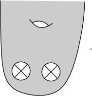
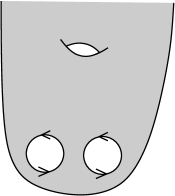
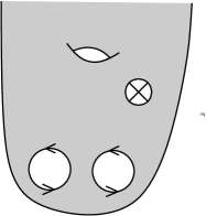
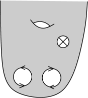
Figure 1: Locally on a Riemann surface, two crosscaps are equivalent to a Klein handle, namely two holes glued together with an orientation reversal. In the presence of a third crosscap somewhere else on the Riemann surface, this is equivalent to an ordinary handle by pulling one of the holes over the auxiliary crosscap.

An alternative point of view on the various string worldsheets is obtained by the so-called doubling construction. A Riemann surface $\Sigma$ as described above (with boundaries, possibly non-orientable) can be viewed as the quotient of an orientable Riemann surface without boundaries $\hat{\Sigma}$ by an orientation reversing involution,

$$\Sigma=\hat{\Sigma}/\Omega$$ (2.6)

(Note that when $\Sigma$ itself is orientable and without boundaries, then $\hat{\Sigma}$ has two connected components exchanged by $\Omega$. The mathematical theory is more uniform, and more familiar, if we temporarily disregard this case.) Inequivalent choices of $\Omega$ lead to different topologies for $\Sigma$. The conformal structure on $\Sigma$ induces a complex structure on $\hat{\Sigma}$ such that $\Omega$ becomes an anti-holomorphic involution. The pair $(\hat{\Sigma},\Omega)$ where $\Omega$ is an anti-holomorphic involution of $\hat{\Sigma}$ is also known as a symmetric Riemann surface. We can think of the moduli space of conformal structures on $\Sigma$ as the moduli space of symmetric Riemann surfaces for this class of $\Omega$.

Let us consider a symmetric Riemann surface $(\hat{\Sigma},\Omega)$, and denote the genus of $\hat{\Sigma}$ by $\hat{g}$. The (negative) Euler character of $\Sigma$ is then given by

$$\chi=\hat{g}-1$$ (2.7)

The number of boundary components of $\Sigma$ is the number of components of the fixed locus, $\Sigma_{\Omega}$, of $\Omega$. Finally, we can identify the index of orientability $k=0,1$ as $2-$(number of connected components of $\hat{\Sigma}\setminus\Sigma_{\Omega}$). These invariants are constrained by the conditions

$$\begin{array}[]{l}\text{1. $0\leq h\leq\hat{g}+1$}\\ \text{2. For $k=0$ (orientable case), $h>0$ and $h\equiv\hat{g}+1\bmod 2$.}\\ \text{3. For $k=1$ (non-orientable case), $0\leq h\leq\hat{g}$.}\\ \end{array}\qquad\qquad$$ (2.8)

Thus, for fixed $\hat{g}$, there are $\lfloor\frac{\hat{g}+2}{2}\rfloor$ orientable worldsheets that can be constructed as quotients $\hat{\Sigma}/\Omega$ and $\hat{g}+1$ non-orientable ones [45] (a modern reference is, e.g., [46]).

To make contact with string perturbation theory, we remember that $\hat{g}=\chi+1$, and that for $\chi$ even, we also have the orientable worldsheet without boundaries of genus $g_{\chi}=\frac{\chi}{2}+1$ (which is not of the form $\hat{\Sigma}/\Omega$ with $\hat{\Sigma}$ connected). Then the total number of worldsheet topologies that appear at order $\chi$ in perturbation theory is

$$\left\lfloor\frac{3\chi+8}{2}\right\rfloor$$ (2.9)

This count of course agrees with the one based on the description using handles, boundaries and crosscaps. We have given the alternative discussion here because it will be helpful further below to understand the various ways in which the various Riemann surfaces can degenerate when we vary the conformal structure.

To organize the following discussion, we find it useful to separate the worldsheets into three classes, depending on whether $c$ is $0$, non-zero and odd, or non-zero and even. We will indicate this by the notation $\Sigma^{(g,h)}$, $\Sigma^{(g,h)_{r}}$, and $\Sigma^{(g,h)_{k}}$, respectively. We shall denote the vacuum amplitudes on oriented surfaces by ${{\cal F}}^{(g,h)}$, those on non-orientable surfaces with an odd number of crosscaps by ${{\cal R}}^{(g,h)}$, and those on non-orientable surfaces with an even number of crosscaps by ${{\cal K}}^{(g,h)}$. The precise meaning of $g$ and $h$ in each case will become clear momentarily.

The total free energy of our topological string is then given by

$${\cal G}=\sum_{\chi}\lambda^{\chi}{{\cal G}}^{(\chi)}$$ (2.10)

where $\lambda$ is the string coupling, and $\chi$ the Euler character of the Riemann surface. ${\cal G}^{(\chi)}$ is given according to the discussion above by

$${{\cal G}}^{(\chi)}=\frac{1}{2^{\frac{\chi}{2}+1}}\Bigl{[}{\cal F}^{(g_{\chi})}+\sum_{2g+h-2=\chi}{{\cal F}}^{(g,h)}+\sum_{2g+h-1=\chi}{{\cal R}}^{(g,h)}+\sum_{2g+h-2=\chi}{{\cal K}}^{(g,h)}\Bigr{]}$$ (2.11)

The first term in this sum is the purely closed string contribution and appears for $\chi$ even, in which case $g_{\chi}=\frac{\chi}{2}+1$.

Before leaving this discussion, we add a remark from [32] concerning the normalization of the topological string amplitudes. General principles of string theory dictate that when we mod out by a symmetry group $G$ of order $|G|$, the amplitude of closed (and orientable) Riemann surface at genus $g$ contributes with a factor of $1/|G|^{g}$ compared to the original theory before modding out. This is to ensure a consistent Hilbert space interpretation in the factorization of loop amplitudes. In our case, $|G|=2$, and $g_{\chi}=\frac{\chi}{2}+1$. This explains the prefactor in (2.11), and we will confirm in section 4 that this is indeed the correct normalization from the point of view of the holomorphic anomaly equation.

Note, however, that a prefactor of $2^{-\frac{\chi}{2}}$ can be reabsorbed in (2.10) by redefining

$${{\cal G}}^{(\chi)}\to 2^{\frac{\chi}{2}}{{\cal G}}^{(\chi)}$$ (2.12)

and the string coupling $\lambda\to\lambda/\sqrt{2}$. It was found in [32] that it is the normalization (2.12) of topological string amplitudes on the resolved conifold that allows for a natural comparison with results in the dual Chern-Simons theory on the deformed conifold. We will confirm in this paper that this normalization is also the correct one for the BPS expansion of topological string amplitudes on compact Calabi-Yau manifolds. It would be interesting to understand this shift of the string coupling more fundamentally.

2.4 Remarks on moduli

The topological amplitudes are functions (or rather, sections of an appropriate bundle) over the moduli space of the underlying conformal field theory. When A- and B-model are decoupled (in the presence of D-branes, we argue that this requires canceling the tadpoles from the respectively “other” model), the amplitudes depend only on the Kähler moduli or complex structure moduli of the underlying Calabi-Yau manifold, respectively. (This dependence is not holomorphic, due to the holomorphic anomaly.) For open strings, we also expect a dependence on open string moduli specifying positions and Wilson line degrees of freedom of the D-branes. A fundamental distinction is that while infinitesimal closed string moduli are never obstructed, open string moduli genuinely are, so it is a priori unclear how to develop an analytic expansion as a function of these parameters. The open string moduli space can be expressed as the critical locus of the superpotential on some appropriate space of massive and massless (infinitesimal) deformations, varying over the moduli space of closed string deformations.

We emphasize again that open string moduli are not generically absent or physically irrelevant. (We don’t want to argue against the important fact that the moduli space of the D0-brane at a point is just the Calabi-Yau manifold itself.) However, it was argued in [8] that, for generic values of the closed string moduli, topological string amplitudes do not depend on any continuous open string moduli, when such are present. We will naturally assume that this statement is true, and that the amplitudes only depend on the discrete moduli. Therefore, if we consider a D-brane configuration with $N$ branes, we will need $N$ discrete labels $v_{1},\ldots v_{N}$ to specify it. (The total number of branes is not naturally fixed, although it is restricted if we impose tadpole cancellation with respect to some given orientifold plane.) The topological amplitudes can then be expanded as

$${{\cal F}}^{(g,h)}(t;v_{1},\ldots,v_{N})=\sum_{i_{1},\ldots i_{h}}{{\cal F}}^{(g,h)}_{v_{i_{1}},\ldots,v_{i_{h}}}(t)$$ (2.13)

where $t$ denotes the closed string moduli. A similar expansion applies to the non-orientable amplitudes, ${{\cal K}}^{(g,h)}$ and ${{\cal R}}^{(g,h)}$.

3 A-model Computations

Localization on the moduli space of stable maps was originally introduced in [23] for the computation of genus $0$ Gromov-Witten invariants on the quintic, and the verification of physicists’ mirror symmetry prediction [47]. Over the years, the method has also been successfully applied for the computation of all-genus (closed) Gromov-Witten invariants in local toric Calabi-Yau manifolds. More recently, the BCOV prediction of genus $1$ Gromov-Witten invariants of hypersurfaces was verified rigorously in [48], with localization as an important tool. In the case of local toric Calabi-Yau manifolds, with toric branes, localization was first used for the computation of open Gromov-Witten invariants in [24], checking the prediction of [22]. The computations were extended to higher genus and multiple boundary components in [25, 26], and to freely acting orientifolds in [27]. In [29], the method was adapted to the computation of open Gromov-Witten invariants on the quintic, with boundary conditions given by the real locus. In this situation, open Gromov-Witten invariants were defined in [49], and the prediction of [29] was then verified rigorously in [30].

We will here combine these various parts, adding a few new ingredients. This will lead to a computation of open Gromov-Witten invariants on the quintic in genus $0$ with an arbitrary number of boundary components, and unoriented Gromov-Witten invariants in genus $1$, again with arbitrary number of boundary components. For local ${\mathbb{P}}^{2}$, with a non-toric brane, we are able to compute these invariants for arbitrary worldsheet topology.

We remark that none of these new invariants (except genus $0$, with one boundary component) has yet been defined rigorously. As a consequence, we have to give some ad-hoc prescriptions how to deal with certain non-isolated fixed loci that occur in the localization process, as well as how to fix the signs related to the orientation of moduli spaces. The latter can probably be determined along the lines of [49, 50], while the former problem should be dealt with by methods similar to those used in [30]. We leave this for future research.

Let us emphasize one aspect of our results which marks a significant departure from the previous works we have mentioned. In those cases, the localization results actually depend on certain of the torus weights. This dependence is due to the need of choosing certain boundary conditions in the space of stable maps [50], and can be related to the framing ambiguity of knots in Chern-Simons theory [51, 52]. As a consequence, the resulting numbers are not truly invariants of the space with D-brane on top, although in all cases they do satisfy the integrality predictions of [22, 31]. In the cases of our interest, we find actual invariant, weight-independent localization results, which however do not satisfy integrality worldsheet by worldsheet. Integrality is recovered once we sum over all worldsheet topologies at fixed order in string perturbation theory. Summing over worldsheet topologies is related to eliminating the boundaries in moduli space, which explains why we obtain an invariant result. We will return to this in section 4.

3.1 The examples

We consider three examples of Calabi-Yau manifolds, $X$: the quintic, the bicubic, and local ${\mathbb{P}}^{2}$. In the first two cases, we fix a particular choice of complex structure. Each of the three examples will be equipped with an anti-holomorphic involution $\sigma:X\to X$. The fixed locus $L$ of $\sigma$ can either be turned into an A-brane by specifying a flat line bundle on top of it, or it can arise as the O-plane in an orientifold model based on $(X,\sigma)$. Later on, we will be interested in giving $L$ both roles simultaneously.

The A-model of course should not depend on the choice of complex structure. In particular, once we equip $L$ with a flat line bundle, we obtain an object in the Fukaya category of $X$ which remains invariant as we vary the complex structure of $X$. For example, the open Gromov-Witten invariants on the disk defined in [49] do not depend on the complex structure, as discussed in [30]. However, it should be noted that once we deform away from the initial complex structure, $L$ need not be the fixed point of an anti-holomorphic involution any longer.

Once we orientifold, the complex structure is actually restricted to be invariant under complex conjugation. Moreover, the topology and homology class of the orientifold plane change along singular conifold loci in the moduli space. (See, [53, 54] for a study of this phenomenon.) By combining this with the remarks from the previous paragraph, we learn that to maintain tadpole cancellation, new branes will have to be created when moving through these singular loci, as discussed in the superstring context in [54]. It will be interesting to study the implications of this for Gromov-Witten theory and BPS invariants.

More specifically, the examples are as follows. The quintic is the vanishing locus of a degree $5$ polynomial in ${\mathbb{P}}^{4}$. Consider the Fermat case

$$\{x_{1}^{5}+x_{2}^{5}+x_{3}^{5}+x_{4}^{5}+x_{5}^{5}=0\}\subset{\mathbb{P}}^{4}$$ (3.1)

This is invariant under complex conjugation $x_{i}\to\bar{x}_{i}$ on ${\mathbb{P}}^{4}$. The fixed point locus $L=\{x_{i}=\bar{x}_{i}\}$ is topologically equal to ${\mathbb{R}}{\mathbb{P}}^{3}$, and admits two choices of flat line bundles. The corresponding discrete Wilson line will be denoted by $\epsilon=\pm 1$. For the localization computation, it is useful to change coordinates such that complex conjugation acts in a non-standard way

$$\sigma:(x_{1},x_{2},x_{3},x_{4},x_{5})\to(\bar{x}_{2},\bar{x}_{1},\bar{x}_{4},\bar{x}_{3},\bar{x}_{5})\,,$$ (3.2)

which is what we have in mind in the following.

The bicubic is the intersection of two cubic polynomials in ${\mathbb{P}}^{5}$. For appropriate choice of complex structure, e.g.,

$$\{x_{1}^{3}+x_{2}^{3}+x_{3}^{3}=0\}\cap\{x_{4}^{3}+x_{5}^{3}+x_{6}^{3}=0\}\subset{\mathbb{P}}^{5}$$ (3.3)

the real locus is also an ${\mathbb{R}}{\mathbb{P}}^{3}$. Again, we switch to coordinates such that complex conjugation acts as

$$\sigma:(x_{1},x_{2},x_{3},x_{4},x_{5},x_{6})\to(\bar{x}_{2},\bar{x}_{1},\bar{x}_{4},\bar{x}_{3},\bar{x}_{6},\bar{x}_{5})$$ (3.4)

Finally, local ${\mathbb{P}}^{2}$ is the total space of the canonical bundle over the projective plane,

$${\cal O}_{{\mathbb{P}}^{2}}(-3)\to{\mathbb{P}}^{2}$$ (3.5)

We take complex conjugation to act as

$$\sigma:(x_{1},x_{2},x_{3})\to(\bar{x}_{2},\bar{x}_{1},\bar{x}_{3})$$ (3.6)

on ${\mathbb{P}}^{2}$ and by complex conjugation in the fiber. The real locus in this case is the total space of the orientation bundle over ${\mathbb{R}}{\mathbb{P}}^{2}$. As before, $H_{1}(L;{\mathbb{Z}})\cong{\mathbb{Z}}_{2}$, so we again have a choice of discrete Wilson line.

For comparison with previous work, we will also evaluate our localization formulas for the conifold, the total space of ${\cal O}(-1)\oplus{\cal O}(-1)$ over ${\mathbb{P}}^{1}$. The brane is the real locus which is isomorphic to the direct sum of two Möbius strips over ${\mathbb{R}}{\mathbb{P}}^{1}$, in other words $S^{1}\times{\mathbb{R}}^{2}$. This is the brane originally studied in [22]. In distinction to the previous cases, $H_{1}(L;{\mathbb{Z}})\cong{\mathbb{Z}}$. This entails further dependence of the localization results on certain torus weights, as in [24]. To eliminate boundaries of moduli space and obtain an invariant result, we have to sum not only over worldsheet topologies, but also over the boundary degree modulo $2$, as was done in [30]. This weight-independence of conifold results is similar to [27], although in that work the orientifold involution was taken to be freely acting.

3.2 Localization

Each of the three examples presented in the previous subsection comes with the natural action of a torus ${\mathbb{T}}^{n}$ on ${\mathbb{P}}^{n-1}$, where $n=5,6,3$ for quintic, bicubic, and local ${\mathbb{P}}^{2}$, respectively. The complex conjugation is compatible with a subtorus ${\mathbb{T}}^{n^{\prime}}$ with $n^{\prime}=2,3,1$, respectively, which is most obvious when complex conjugation is taken to act as in (3.2), (3.4), (3.6). In each case, we have a canonical lift of the ${\mathbb{T}}^{n}$ action to the bundles ${\cal O}_{{\mathbb{P}}^{n-1}}(k)$ compatible with the real structure. The conifold is invariant under ${\mathbb{T}}^{3}$, and its real brane is compatible with a ${\mathbb{T}}^{2}\subset{\mathbb{T}}^{3}$. In this way, the real brane of the conifold is actually identical to one of the “toric” branes that have been much studied in the literature, starting with [51].

Following the cited literature, we consider moduli spaces of maps of degree $d$ from a worldsheet $\Sigma$ of one of the topological types $(g,h)$, $(g,h)_{r}$, or $(g,h)_{k}$ discussed in section 2 to the ambient target space ${\mathbb{P}}^{n-1}$, with some extra data, as follows. When $\Sigma$ is orientable with non-empty boundary, we require that the boundary be mapped to the real locus. Note that any such map can be completed to an invariant map from the doubled surface $\hat{\Sigma}$ to ${\mathbb{P}}^{n-1}$. So more uniformly, whether $\Sigma$ is orientable or not, we can think of a map from the doubled worldsheet $\hat{\Sigma}\to{\mathbb{P}}^{n-1}$ that is equivariant with respect to the action of $\Omega$ (where $\Sigma=\hat{\Sigma}/\Omega$) on $\hat{\Sigma}$ and complex conjugation $\sigma$ on the target space. The fixed points of $\Omega$ are automatically mapped to the Lagrangian brane. Since we have in mind a fixed boundary condition and orientifold projection in all cases, we denote the moduli space simply by

$${\cal M}_{\Sigma}({\mathbb{P}}^{n-1},d)$$ (3.7)

and we reserve technicalities associated with the proper compactification of these spaces for a later discussion.

We now come to an important point. As we just mentioned, any boundary of $\Sigma$ is automatically mapped to the Lagrangian $L$, but we have so far not specified its homology class in $H_{1}(L)$, which is $\cong{\mathbb{Z}}_{2}$ in all three cases of interest. When that class is trivial, then under deformation of the map (or under change of complex structure of the target space, for the quintic and bicubic), it can happen that the boundary is collapsed to a point on $L$. This is one of the real codimension-one boundaries in the moduli space that we have been warned about. As we will see, it is the only dangerous one, at least in the examples we consider here. From the doubled perspective, $\hat{\Sigma}$ develops a node that lies right on top of the Lagrangian $L$. Reflection shows that such a real nodal curve admits another smoothing to a curve that is equivariant, but with respect to a different anti-holomorphic involution of $\hat{\Sigma}$, that locally looks like a crosscap.

The local model of this phenomenon is the map ${\mathbb{P}}^{1}\ni(u,v)\mapsto(x,y,z)\in{\mathbb{P}}^{2}$ defined by

$$\begin{split}x&=au^{2}\\ y&=av^{2}\\ z&=uv\end{split}$$ (3.8)

where $a$ is a parameter. The image of the map is the conic

$$xy-a^{2}z^{2}=0$$ (3.9)

Whenever $a^{2}\in{\mathbb{R}}$, the image curve is real under $(x,y,z)\mapsto(\bar{y},\bar{x},\bar{z})$, but for the map (3.8) to be equivariant, we have to choose the involution to act on ${\mathbb{P}}^{1}$ as

$$\begin{split}(u,v)&\mapsto(\bar{v},\bar{u})\;\;\;\qquad a\in{\mathbb{R}}\\ (u,v)&\mapsto(\bar{v},-\bar{u})\qquad a\in{\it i}{\mathbb{R}}\end{split}$$ (3.10)

In the first case, we obtain a map from the disk to ${\mathbb{P}}^{2}$ with boundary on ${\mathbb{R}}{\mathbb{P}}^{2}$, in the second case we obtain a map from the crosscap to the orientifold. Thus, we see that as we vary the (target space) parameter $a^{2}$, we can have transitions where we loose holomorphic disks and gain holomorphic crosscaps. Since this is a local phenomenon, happening in real codimension $1$, the only way to account for this process is to count disks with collapsible boundaries and crosscaps together. Deferring a more careful discussion to a later stage, we are now ready to explain how we will do the computations. We temporarily assume that any boundary component is mapped to a non-trivial homology class in $H_{1}(L)$.

We intend to compute Gromov-Witten invariants, $\tilde{n}^{\Sigma}_{d}$, by integrating over the moduli space ${\cal M}_{\Sigma}({\mathbb{P}}^{n-1},d)\ni f$ the top Chern class of an appropriate bundle ${\cal E}_{d}$. In the three cases, we have

$${\cal E}_{d}=\begin{cases}H^{0}(\Sigma,f^{*}{\cal O}(5))&X={\rm quintic}\\ H^{0}(\Sigma,f^{*}{\cal O}(3)^{\oplus 2})&X={\rm bicubic}\\ H^{1}(\Sigma,f^{*}{\cal O}(-3))&X=\text{local ${\mathbb{P}}^{2}$}\end{cases}$$ (3.11)

Namely, we assume that for each topological type of surface, we will have an Euler class formula of the form

$$\tilde{n}_{d}^{\Sigma}=\int_{{\cal M}_{\Sigma}({\mathbb{P}}^{n-1},d)}{\bf e}({\cal E}_{d})$$ (3.12)

which we will evaluate by using Atiyah-Bott localization following the cited literature.

As explained in [23], the fixed loci of the action of ${\mathbb{T}}^{n}$ are nodal curves in which any node or any component of non-zero genus is collapsed to one of the fixed points in target space, and any non-contracted rational component is mapped on one of the coordinate lines with a standard map of a certain degree. The components of the fixed locus can be represented by a decorated graph,

$$\Gamma=\{v_{1},\ldots,v_{k};e_{1},\ldots,e_{l};p_{1},\ldots,p_{k};g_{1},\ldots,g_{k};d_{1},\ldots,d_{l}\}$$ (3.13)

The graph data consists of a set of vertices $(v_{i})_{i=1,\ldots,k}$, and a set of edges $(e_{j})_{j=1,\ldots,l}$. The decoration consists of the genus $g_{i}\geq 0$ of any contracted component at the $i$-th vertex, the target space fixed points $1\leq p_{i}\leq n$ to which that component is mapped, and the degree $d_{j}$ of the maps from the edges to the corresponding coordinate line. We will conveniently omit the decorations $g_{i}=0$ and $d_{j}=1$.

We are here interested in localization with respect to ${\mathbb{T}}^{n^{\prime}}$ on the space of real maps, i.e., maps equivariant with respect to conjugation on target and worldsheet

$$(\hat{\Sigma},\Omega)\to(X,\sigma)$$ (3.14)

Initially, we will fix the topological type of $\Sigma=\hat{\Sigma}/\Omega$, as well as the homology class of any boundary component of $\Sigma$. We will always fix the total degree of the map, which in terms of the graph data is given by $d=\sum d_{i}$, as well as the total genus of $\hat{\Sigma}$, which is determined by $\hat{g}=1-k+l+\sum g_{i}$. The target space involution $\sigma$ is determined by (3.2), (3.4), (3.6), respectively, and acts only on the decoration $\{p_{i}\}$. The involution on the domain is specified by a map on vertices and edges that is compatible with the decoration by genus and degree. Moreover, for any fixed edge, we have to specify whether the involution acts by $z\to 1/\bar{z}$ or $z\to-1/\bar{z}$ on the inhomogeneous coordinate of the corresponding rational curve [27]. The topological type of $\Sigma$ and the map can easily be recovered from this data.

Instead of thinking of the equivariant map (3.14), represented by a real graph. we can also think of a “half-map” $\Sigma\to X/\sigma$, and accordingly remember only half of the graph, as well as how it is reflected. This is algorithmically more economical, however one has to be extra careful with identifying automorphisms of the graph (see below).

The localization formula then takes the form

$$\tilde{n}^{\Sigma}_{d}=(-1)^{p(\Sigma)}\sum_{\Gamma}\frac{1}{|\mathop{\rm Aut}\Gamma|}\int_{{\cal M}_{\Gamma}}\frac{{\bf e}({\cal E}_{d})}{{\bf e}({\cal N}_{\Gamma})}$$ (3.15)

where the sum is over all real graphs (or half-graphs) of the appropriate type. Here, ${\cal M}_{\Gamma}$ is the component of the fixed locus that corresponds to $\Gamma$, and ${\cal N}_{\Gamma}$ is the corresponding normal bundle. Depending on one’s point of view, the bundles in (3.15) are either the real bundles pulled back via the equivariant map, or the complex bundles pulled back via the half-maps. The ${\bf e}$’s in (3.15) are the equivariant Euler classes. We have reserved a sign $(-1)^{p(\Sigma)}$ to be able to adjust the relative orientation between moduli spaces of maps from different worldsheet topologies. This will become important when we sum over the worldsheet topologies at fixed Euler characteristic.

To proceed, we will borrow the formulas for the tangent and obstruction weights from the cited literature. The signs of the Euler classes coming from disk components are documented in [30], but there will be additional signs associated with crosscaps and unoriented loops that we will discuss below [27]. An issue that will require renewed attention is the appearance of zero weight components when the torus weights are specialized from ${\mathbb{T}}^{n}$ to ${\mathbb{T}}^{n^{\prime}}$. One of the results of this discussion will be that we will never perform integrals over moduli spaces of real curves (contracted to a $\sigma$- and ${\mathbb{T}}^{n^{\prime}}$-invariant point in target space). The remaining integrals over ${\cal M}_{\Gamma}$ are performed using Faber’s algorithm [55]. But before we get into all these subtleties, and to get oriented about the notation, it will be helpful to first discuss a few simple cases. Incidentally, this will immediately reveal the fundamental puzzle with the BPS interpretation of these invariants, as well as suggest the possible resolution.

One last thing. In the complex case, the localization formula applies in higher genus only for $X=\text{local ${\mathbb{P}}^{2}$}$. For hypersurfaces, the formula is only valid in genus $0$, and the methods of [48] have to be invoked in higher genus. In the real case, it turns out that because of the restriction on the degree of the boundary components, and the generous treatment of real torus fixed points, we can actually evaluate certain classes of higher-genus curves using the naive expressions also on the quintic and bicubic.

So consider the degree $2$ invariant of the annulus, with both boundary components non-trivial in $H_{1}(L)$. It is easy to see that (before decoration) there is only type of graph, shown in Fig. 2. It is straightforward to evaluate the sum (3.15), and one finds

$$\begin{array}[]{c|c|c|c}&{\rm quintic}&{\rm bicubic}&\text{local ${\mathbb{P}}^{2}$}\\ \hline\cr\tilde{n}^{(0,2)}_{2}&-\frac{45}{8}&-\frac{9}{8}&\frac{3}{8}\end{array}$$ (3.16)

It is clear that this result is incompatible with the BPS interpretation expected from [22, 31]. One of the features of these multi-cover formulas is that the number of boundary components is fixed. In particular, no curves of lower genus bubble onto annuli in degree $2$. What is worse, the double of the annulus of degree $2$ would be an elliptic curve of degree $2$. But projective space has no such curves! So the (integral) invariant $n^{(1,{\rm real})}_{2}$ should actually vanish.

Figure 2: Left: The only fixed graph contributing to the annulus invariant $\tilde{n}^{(0,2)}_{2}$ in degree $2$. Right: The doubled graph can also contribute to the Klein bottle invariant $\tilde{n}^{(1,0)_{k}}_{2}$. In the latter case, the involution $\Omega$ exchanges the two lines as indicated.

The most conservative way to reconcile the situation is to realize that the doubled graph corresponding to our annulus is also equivariant with respect to a different involution on the worldsheet curve, yielding a Klein bottle in the quotient (see right of fig. 2). The weights are equal to those of the annulus, and we identify the signs such that the two contributions exactly cancel. At the level of graphs, such a cancellation was first described in [27], but because of a different involution in target space, was interpreted there as a cancellation among Klein bottles.

3.3 Homologically trivial boundaries, and local tadpole cancellation

After this initial success, let us briefly return to the computations in [29, 49, 30]. In these works, disk invariants $\tilde{n}^{(0,1)}_{d}$ on the quintic were computed for all odd degrees $d\in 2{\mathbb{Z}}+1$. It was also noted that disk invariants of even degree are either ill-defined because of mixing with non-orientable worldsheets (crosscaps) or else vanish because the moduli space is odd-dimensional, and hence any well-defined Euler class would be trivial.

Graphically, one can understand this vanishing as follows. Consider a localization graph with a fixed edge of even degree, equal to $2$ in Fig. 3.

Figure 3: A localization graph with a fixed edge of even degree always contributes equal amounts to a real Gromov-Witten invariant for a worldsheet where $\Omega$ acts on that edge with fixed points (a boundary), or without (a crosscap). The signs in the localization calculus are such that those contributions exactly cancel.

Following the localization prescription, the involution on $\hat{\Sigma}$ can act on this fixed edge either by $z\to 1/\bar{z}$ or $z\to-1/\bar{z}$, resulting in a disk or crosscap component, respectively. We had decided earlier that to get an invariant count of real curves, we should combine such contributions. The best sign is such that they exactly cancel, in agreement with the previous argument.

In the computations below, we have extended this prescription to any $\Omega$-fixed edge of even degree. The vanishing of the $\text{(homologically trivial disk)}+\text{crosscap}$ contribution to the total invariant can be viewed as the microscopic realization, graph by graph, of tadpole cancellation, which we will discuss in more detail below. Note that our prescription also temporarily addresses the problem that the contribution to the equivariant Euler formula from such an even degree edge contains (for $n$ odd) a factor $\frac{0}{0}$ and is hence a priori ambiguous. We will return to this below.

So let us assume that real graphs with any fixed edge of even degree always cancel after summing over different worldsheet involutions. We will also assume (and justify later) that graphs with an $\Omega$-invariant vertex mapping to a $\sigma$- and ${\mathbb{T}}^{n^{\prime}}$-invariant point in ${\mathbb{P}}^{n-1}$ (those exist for $n$ odd) do not contribute. As a consequence of this, we compute non-vanishing invariants $\tilde{n}^{(g,h)}_{d}$ by summing over “orientable half-graphs” of genus $g$ with $h$ ($h>0$) boundary components of odd degree. These correspond to real graphs of genus $\hat{g}=2g+h-1$ that are disconnected when cut along the $h$ fixed edges. We denote by $\tilde{n}^{(g,h)_{k}}_{d}$ invariants obtained from real graphs with $\hat{g}=2g+h-1$ that remain connected after cutting along $h$ fixed edges of odd degree. (In this case, $h$ can be zero, cf., eq. (2.8).) The total degree is seen to satisfy $d\equiv h\bmod 2$. All other combinations of topological invariants lead to a vanishing sum over graphs. For future reference we record the selection rule

$$d\equiv h\equiv\chi\bmod 2$$ (3.17)

where we recall that negative $\chi$ is the Euler characteristic of $\Sigma$, related to the genus of the covering curve by $\chi=\hat{g}-1$.

To further clarify these rules, we consider in detail one more example, the annulus/Klein bottle invariants in degree $4$. There are in each case three graphs, see Fig. 4. Note that there are even degree edges at the center of the first Klein bottle graph. However, $\Omega$ acts by exchanging them, so the above vanishing rule does not apply. (See next subsection for more details.)

Figure 4: Localization graphs contributing to annulus invariant $\tilde{n}^{(0,2)}_{4}$ (left) and to the Klein bottle invariant $\tilde{n}^{(1,0)_{k}}_{4}$ (right). In distinction to Figs. 2 and 3, the real graphs are not in one-to-one correspondence, and the sum $\tilde{n}^{(0,2)}_{4}+\tilde{n}^{(1,0)_{k}}_{4}$ does not vanish. (In particular, the graphs on the third line are not identical once the $\sigma$-symmetric decoration is taken into account.)

The annulus graphs sum up to

$$\begin{array}[]{c|c|c|c}&{\rm quintic}&{\rm bicubic}&\text{local ${\mathbb{P}}^{2}$}\\ \hline\cr\tilde{n}^{(0,2)}_{4}&-\frac{15525}{16}&-\frac{585}{16}&-\frac{21}{16}\end{array}$$ (3.18)

while the Klein bottles give

$$\begin{array}[]{c|c|c|c}&{\rm quintic}&{\rm bicubic}&\text{local ${\mathbb{P}}^{2}$}\\ \hline\cr\tilde{n}^{(1,0)_{k}}_{4}&\frac{582725}{16}&\frac{22761}{16}&\frac{117}{16}\end{array}$$ (3.19)

Again, annuli and Klein bottles individually do not make sense from the point of view of integrality, but their sums

$$2n^{(1,{\rm real})}_{4}=\tilde{n}^{(1,0)_{k}}_{4}+\tilde{n}^{(0,2)}_{4}$$ (3.20)

are

$$\begin{array}[]{c|c|c|c}&{\rm quintic}&{\rm bicubic}&\text{local ${\mathbb{P}}^{2}$}\\ \hline\cr 2n^{(1,{\rm real})}_{4}&35450&1386&6\end{array}$$ (3.21)

and integral as advertised.

3.4 Results

We will give the explicit localization formula in terms of the “half-graphs” because they are more economical and the signs can be made more explicit. We will give the weights of the normal bundle only when there are no collapsed components of higher genus (although the total graph might still have non-trivial topology), and the weights of ${\cal E}_{d}$ only for the quintic. The formulas for the bicubic are essentially similar. For local ${\mathbb{P}}^{2}$ (and the conifold) it also makes sense to evaluate graphs with non-trivial genus at the vertices. The corresponding formulas can be constructed from, e.g., [56, 57, 26, 27].

A graph of requisite type can be thought of as an ordinary graph as in say [23] to which is attached a certain number of “half-edges”. Some of these edges represent disks, which requires the corresponding degree to be odd. The other half-edges, which can be of even or odd degree, are identified pairwise, and represent “Klein edges”. This means that the doubled graph is constructed by reflection on the disks and exchange of the pairwise identified half-edges. We can count the Klein edges among ordinary edges by remembering that if they arise from identification of half-edges attached at vertices decorated by $i$ and $j$, then the Klein edge is decorated with $i$ and $\sigma(j)$ at its two ends. (This imposes a restriction on the decoration of the half-graph.) A similar comment applies to collecting the flags associated to the vertices. The contribution of such a graph to the sum (3.15) is then given by

$$\begin{split}\int_{{\cal M}_{\Gamma}}\frac{{\bf e}({\cal E}_{d})}{{\bf e}({\cal N}_{\Gamma})}&=(-1)^{\#{\rm klein}}\prod_{\rm edges}\frac{\displaystyle\prod_{a=0}^{5d}\frac{a\lambda_{i}+(5d-a)\lambda_{j}}{d}}{\displaystyle(-1)^{d}\frac{(d!)^{2}}{d^{2d}}(\lambda_{i}-\lambda_{j})^{2d}\prod_{\genfrac{}{}{0.0pt}{2}{\scriptstyle k\neq i,j}{\scriptstyle a=0}}^{d}\Bigl{(}\frac{a}{d}\lambda_{i}+\frac{d-a}{d}\lambda_{j}-\lambda_{k}\Bigr{)}}\\[5.69046pt] \cdot\prod_{\rm disks}&\frac{\displaystyle\prod_{a=0}^{(5d-1)/2}\frac{a\lambda_{i}+(5d-a)\lambda_{\sigma(i)}}{d}}{\displaystyle(-1)^{(d-1)/2}\frac{d!}{d^{d}}(\lambda_{i}-\lambda_{\sigma(i)})^{d}\prod_{\genfrac{}{}{0.0pt}{2}{\scriptstyle k\neq i,\sigma(i)}{\scriptstyle a=0}}^{(d-1)/2}\Bigl{(}\frac{a}{d}\lambda_{i}+\frac{d-a}{d}\lambda_{\sigma(i)}-\lambda_{k}\Bigr{)}}\\ \cdot\prod_{\rm vertices}&\frac{1}{(5\lambda_{v})^{{\rm val}(v)-1}}\prod_{j\neq v}(\lambda_{v}-\lambda_{j})^{{\rm val}(v)-1}\cdot\biggl{(}\prod_{\rm flags}\frac{d}{\lambda_{v}-\lambda_{j}}\biggr{)}\biggl{(}\sum_{\rm flags}\frac{d}{\lambda_{v}-\lambda_{j}}\biggr{)}^{{\rm val}(v)-3}\end{split}$$ (3.22)

The sign at the beginning of (3.22) measures the number of Klein edges, which agrees with the rules given in [27]. The sign in (3.15) is given by

$$(-1)^{p(\Sigma)}=(-1)^{g+\chi-1}$$ (3.23)

Before summing these results over all decorated graphs, we need to specialize the weights $\lambda_{i}$, $i=1,\ldots,n$ to those invariant under target space involution $\sigma$, cf., (3.2), (3.4), (3.6). For the quintic and local ${\mathbb{P}}^{2}$, this specialization introduces zero weight components in the form of $\frac{0}{0}$, and we must specify some rules to deal with this ambiguity. The origin of these unexpected torus-invariant directions is the existence of real torus fixed points in ${\mathbb{P}}^{n-1}$ for odd $n$. The fixed locus thereby acquires an additional dimension that connects graphs which locally differ as depicted in Fig. 5. (This is the graphical representation of the one-parameter family of maps (3.8).)

Figure 5: Graphs that differ by a local replacement as indicated actually belong to a one-dimensional fixed locus.

When the edge in question is fixed under the involution, the moduli space is real one-dimensional, and our rules on tadpole cancellation imply a vanishing contribution. When the edge is not fixed under $\Omega$, our rule is that the complex one-dimensional moduli space gives a non-zero contribution that can be taken either from the left or the right graph in the figure.

Using this algorithm, we have evaluated the sums (3.15) for a certain number of worldsheet topologies and first few non-trivial degrees in each case. We summarize the results in the following tables. We also give results for the conifold, that has been analyzed previously in [24, 25, 26]. In particular, $\nu$ is the choice of torus weights in the fiber of ${\cal O}(-1)\oplus{\cal O}(-1)$. Our convention is related to the standard framing ambiguity via

$$\nu=2\nu_{\rm framing}-1$$ (3.24)

There is a symmetry under $\nu\to-\nu$, or $\nu_{\rm framing}\to 1-\nu_{\rm framing}$, hence the results are polynomials in $\nu^{2}$.

$$\begin{array}[]{|cc||c|c|c|c||}\hline\cr&d&{\rm quintic}&{\rm bicubic}&\text{local ${\mathbb{P}}^{2}$}&{\rm conifold}\\ \hline\cr\tilde{n}^{(0,2)}_{d}&2&-\frac{45}{8}&-\frac{9}{8}&\frac{3}{8}&-\frac{1}{8}(1-\nu^{2})\\ &4&-\frac{15525}{16}&-\frac{585}{16}&-\frac{21}{16}&-\frac{1}{16}(1-\nu^{4})\\ &6&-\frac{6387015}{4}&-\frac{123501}{8}&\frac{59}{4}&-\frac{1}{24}(1-\nu^{6})\\ &8&-\frac{66757119525}{32}&-\frac{150570441}{32}&-\frac{5781}{32}&-\frac{1}{32}(1-\nu^{8})\\ \hline\cr\tilde{n}^{(1,0)_{k}}_{d}&2&\frac{45}{8}&\frac{9}{8}&-\frac{3}{8}&\frac{1}{8}(1-\nu^{2})\\ &4&\frac{582725}{16}&\frac{22761}{16}&\frac{117}{16}&\frac{1}{16}(1-\nu^{4})\\ &6&\frac{295022375}{4}&\frac{6234093}{8}&-\frac{411}{4}&\frac{1}{24}(1-\nu^{6})\\ &8&\frac{4250971393125}{32}&\frac{10876810761}{32}&\frac{48981}{32}&\frac{1}{32}(1-\nu^{8})\\ \hline\cr\hline\cr\end{array}$$

Table 1: Localization invariants at $\chi=0$.

$$\begin{array}[]{|cc||c|c|c|c||}\hline\cr&d&{\rm quintic}&{\rm bicubic}&\text{local ${\mathbb{P}}^{2}$}&{\rm conifold}\\ \hline\cr\tilde{n}^{(0,3)}_{d}&3&\frac{45}{16}&\frac{3}{16}&-\frac{3}{16}&\frac{1}{48}(1-2\nu^{2}+\nu^{4})\\ &5&\frac{5175}{8}&\frac{117}{16}&\frac{9}{8}&\frac{1}{48}(1-3\nu^{4}+2\nu^{6})\\ &7&\frac{36429885}{16}&\frac{58851}{8}&-\frac{333}{16}&\frac{1}{48}(1-4\nu^{6}+3\nu^{8})\\ \hline\cr\tilde{n}^{(1,1)}_{d}&1&&&\frac{1}{12}&-\frac{1}{12}\\ &3&&&-\frac{3}{8}&-\frac{1}{24}(1+2\nu^{2}-\nu^{4})\\ &5&&&\frac{3}{4}&-\frac{1}{24}(1+3\nu^{4}-2\nu^{6})\\ &7&&&\frac{839}{24}&-\frac{1}{24}(1+4\nu^{6}-3\nu^{8})\\ \hline\cr\tilde{n}^{(1,1)_{k}}_{d}&3&-\frac{135}{16}&-\frac{9}{16}&\frac{9}{16}&-\frac{1}{16}(1-2\nu^{2}+\nu^{4})\\ &5&-\frac{866325}{8}&-\frac{22527}{16}&-\frac{171}{8}&-\frac{1}{16}(1-3\nu^{4}+2\nu^{6})\\ &7&-\frac{5109042135}{16}&-\frac{9054153}{8}&\frac{7047}{16}&-\frac{1}{16}(1-4\nu^{6}+3\nu^{8})\\ \hline\cr\hline\cr\end{array}$$

Table 2: Localization invariants at $\chi=1$.

$$\begin{array}[]{|cc||c|c|c|c||}\hline\cr&d&{\rm quintic}&{\rm bicubic}&\text{local ${\mathbb{P}}^{2}$}&{\rm conifold}\\ \hline\cr\tilde{n}^{(0,4)}_{d}&4&-\frac{135}{64}&-\frac{3}{64}&\frac{9}{64}&-\frac{1}{192}(1-\nu^{2})^{3}\\ &6&-\frac{46575}{128}&-\frac{117}{128}&-\frac{135}{128}&-\frac{1}{128}(1-\nu^{2})^{3}(1+3\nu^{2})\\ &8&-\frac{105398415}{32}&-\frac{113931}{32}&\frac{945}{32}&-\frac{1}{96}(1-\nu^{2})^{3}(1+3\nu^{2}+6\nu^{4})\\ \hline\cr\tilde{n}^{(1,2)}_{d}&2&&&-\frac{5}{128}&\frac{1}{384}(1-\nu^{2})(9-\nu^{2})\\ &4&&&\frac{41}{64}&\frac{1}{192}(1-\nu^{2})(4+21\nu^{2}-9\nu^{4})\\ &6&&&-\frac{81}{128}&\frac{1}{384}(1-\nu^{2})(12+12\nu^{2}+119\nu^{4}-71\nu^{6})\\ \hline\cr\tilde{n}^{(1,2)_{k}}_{d}&4&\frac{405}{32}&\frac{9}{64}&-\frac{27}{32}&\frac{1}{32}(1-\nu^{2})^{3}\\ &6&\frac{15454125}{64}&\frac{66879}{64}&\frac{2997}{64}&\frac{3}{64}(1-\nu^{2})^{3}(1+3\nu^{2})\\ \hline\cr\tilde{n}^{(2,0)_{k}}_{d}&2&&&\frac{5}{128}&-\frac{1}{384}(1-\nu^{2})(9-\nu^{2})\\ &4&&&\frac{33}{16}&-\frac{1}{192}(1-\nu^{2})(9+11\nu^{2}-4\nu^{4})\\ &6&&&-\frac{10953}{64}&-\frac{1}{384}(1-\nu^{2})(27+27\nu^{2}+44\nu^{4}-26\nu^{6})\\ \hline\cr\hline\cr\end{array}$$

Table 3: Localization invariants at $\chi=2$.

$$\begin{array}[]{|cc||c|c|c|c||}\hline\cr&d&{\rm quintic}&{\rm bicubic}&\text{local ${\mathbb{P}}^{2}$}&{\rm conifold}\\ \hline\cr\tilde{n}^{(0,5)}_{d}&5&\frac{2025}{1024}&\frac{15}{1024}&-\frac{135}{1024}&\frac{5}{3072}(1-\nu^{2})^{4}\\ &7&0&-\frac{1911}{5120}&\frac{1323}{1280}&\frac{49}{15360}(1-\nu^{2})^{4}(1+4\nu^{2})\\ &9&\frac{2510008965}{512}&\frac{2271807}{1280}&-\frac{10935}{256}&\frac{27}{5120}(1-\nu^{2})^{4}(1+4\nu^{2}+10\nu^{4})\\ \hline\cr\tilde{n}^{(1,3)}_{d}&3&&&\frac{3}{128}&-\frac{1}{1152}(1-\nu^{2})^{2}(11-2\nu^{2})\\ &5&&&-\frac{309}{256}&-\frac{1}{2304}(1-\nu^{2})^{2}(25+218\nu^{2}-93\nu^{4})\\ \hline\cr\tilde{n}^{(2,1)}_{d}&1&&&-\frac{7}{2880}&\frac{7}{2880}\\ &3&&&\frac{79}{2880}&\frac{8+120\nu^{2}-75\nu^{4}+10\nu^{6}}{2880}\\ &5&&&-\frac{59}{128}&\frac{15-48\nu^{2}+324\nu^{4}-284\nu^{6}+63\nu^{8}}{1152}\\ \hline\cr\tilde{n}^{(1,3)_{k}}_{d}&5&-\frac{10125}{512}&-\frac{75}{512}&\frac{675}{512}&-\frac{25}{1536}(1-\nu^{2})^{4}\\ &7&-\frac{7816725}{16}&-\frac{360297}{512}&-\frac{11907}{128}&-\frac{49}{1536}(1-\nu^{2})^{4}(1+4\nu^{2})\\ \hline\cr\tilde{n}^{(2,1)_{k}}_{d}&3&&&-\frac{9}{128}&\frac{1}{384}(1-\nu^{2})^{2}(11-2\nu^{2})\\ &5&&&-\frac{12723}{1024}&\frac{(1-\nu^{2})^{2}(225+622\nu^{2}-247\nu^{4})}{3072}\\ \hline\cr\hline\cr\end{array}$$

Table 4: Localization invariants at $\chi=3$.

All these results are compatible with integrality by using the appropriate multi-cover formula, see section 5. The feature of the conifold results is that the sum over worldsheet topologies with fixed $\chi$ yields a $\nu$-independent answer that agrees with the multi-cover formula originally conjectured in [22]. This weight-independence is similar to that noticed for freely acting orientifold in [27].

4 Formal Developments

The results of the localization computations of the previous section suggest that we study the topological string in the presence of both D-branes and orientifolds, and give an enumerative or BPS interpretation only to the total topological string amplitude. In our examples, in the A-model, the D-brane and the orientifold plane are wrapped on the same Lagrangian, given as the fixed point set of an anti-holomorphic involution. If it makes sense however, wrapping the same Lagrangian should not be a necessary restriction. For example, we know already that disk instantons deform the (superpotential on the) Lagrangian viewed as D-brane [29], whereas the vanishing result for holomorphic crosscaps shows that the same Lagrangian viewed as orientifold plane is not corrected. The natural invariant statement is that we should have a similar interpretation of $\text{open}+\text{unoriented}$ topological string amplitudes whenever the D-brane is wrapped in the same homology class as the orientifold plane.

In this section, we will study consequences of this assumption. In particular, we will write down holomorphic anomaly equations for topological string amplitudes on the general open and non-orientable worldsheet, extending [2, 8]. In the next section, we will return to the example and use these holomorphic anomaly equations to reproduce and extend the A-model results in the B-model.

4.1 The tadpole state as a normal function

We begin the discussion at tree level. Consider the compactification of the type I string (or type IIB orientifold) on a Calabi-Yau manifold $Y$, and recall from [58] the formula for the 4-d space-time superpotential

$${\cal W}=\int_{Y}H\wedge\Omega\,,$$ (4.1)

where $\Omega$ is the holomorphic three-form and $H$ the RR $3$-form field strength. As emphasized in [33], this formula is best viewed as expressing the fact that the superpotential ${\cal W}$ is “generated by D5-brane charge”, in the following sense. When the background contains only D5-branes and O5-planes wrapped on a collection of holomorphic curves $C=\sum_{i}C_{i}$, tadpole cancellation requires that the total homology class vanishes, $[C]=\sum_{i}[C_{i}]=0\in H_{2}(Y)$. There is then a three-chain $\Gamma$ with boundary $\partial\Gamma=C$, and the formula (4.1) becomes

$${\cal W}=\int_{\Gamma}\Omega$$ (4.2)

In the presence of O9-planes and D9-branes wrapped on the Calabi-Yau with some choice of gauge bundle, the formula (4.1) includes a contribution from the holomorphic Chern-Simons functional [59], evaluated at the critical point (i.e., the gauge bundle is holomorphic). This can again be represented in the form (4.2) for appropriate choice of $C=\partial\Gamma$. Integrals of the form (4.2) are related [43, 8] to what are known mathematically as “Poincaré normal functions”.

From the holomorphic point of view, the formula (4.2) can be understood as arising from a computation of the topological string amplitude on the disk and crosscap (${\mathbb{R}}{\mathbb{P}}^{2}$) [32, 33]. This computation is well-defined, and representable geometrically by (4.2), whenever the total topological D-brane charge vanishes. Note that in computing the topological charge of the orientifold plane, one has to take into account that it fills $d=4$-dimensional space-time. This imparts an extra factor of $2^{d/2}=4$ to the O-plane charge.

To make this more tangible, it is convenient to temporarily switch to the A-model on the mirror Calabi-Yau $X$. In this case, D-brane charges are just homology classes in $H_{3}(X;{\mathbb{Z}})$. The corresponding type IIA setup contains an O6-plane, which carries $4$ units of D6-brane charge (as viewed from the covering space. The gauge group on a tadpole canceling D6-brane configuration on top of the O6-plane is $SO(4)$.)

In the previous section, we have seen that to obtain a satisfactory integral BPS expansion of the topological amplitudes, computed via localization in the A-model, we should sum worldsheets of different topology, at fixed order in string perturbation theory. In forming this sum, different number of boundaries simply contribute with a unit weight, see e.g., (3.20). This means that the background contains just a single D-brane in the covering space. In other words, for purposes of tadpole cancellation in the topological string, the charge of the topological orientifold plane is simply equal to its homology class. This value of the topological O-plane charge agrees with that identified in [32] by duality with ${\it SO}$/${\it Sp}$-Chern-Simons theory.

An elementary way to compute the topological O-plane charge is to use the parity twisted Witten index of the underlying ${\cal N}=2$ worldsheet theory. Recall that the Witten index in the open string sector between branes $B$ and $B^{\prime}$ can be computed by an index theorem as an appropriate inner product of the corresponding D-brane charges [60],

$${\rm Tr}_{{\cal H}_{B,B^{\prime}}}(-1)^{F}=\langle{\rm ch}(B),{\rm ch}(B^{\prime})\rangle$$ (4.3)

Now given an orientifold defined by a parity $P$, the O-plane charge ${\rm ch}(\text{O-plane})$ is defined by requiring that the parity twisted Witten index in the open string sector between any brane $B$ and its parity image $P(B)$ satisfy

$${\rm Tr}_{{\cal H}_{B,P(B)}}P(-1)^{F}=\langle{\rm ch}(B),{\rm ch}(\text{O-plane})\rangle$$ (4.4)

In the A-model, the formulas (4.3) and (4.4) reduce simply to the geometric intersection indices between the corresponding three-cycles, which justifies the above value of the O-plane charge.

To embed this in the superstring, we should consider a situation in which the charge of the orientifold plane is equal to that of the corresponding D-brane. To achieve this, we need to switch from the O6/D6-setup of a type I/II compactification discussed above, to a situation in which we have O4-planes/D4-branes wrapped on the 3-cycle, and extended along a $2$-dimensional subspace of Minkowski space. Remarkably enough, this is exactly the situation in which we are expecting a BPS interpretation of open and unoriented topological string amplitudes [22, 32]. We have thus completed the circle of observations that began with the A-model results in the previous section.

This connection of our findings on tadpole cancellation with the superstring setup is quite satisfying, but also raises some intriguing questions. First of all, it is not immediately clear why the physical setup with O4/D4 requires cancellation of RR-tadpoles, because the transverse space is still non-compact. To address this, note that from the 4d-perspective, the O/D-string carries axionic charge under the appropriate fields from the ${\cal N}=2$ hypermultiplets, while the BPS states on the string (that are counted by the topological string amplitudes) are charged under the vectormultiplets. Thus the need to cancel the tadpoles might indicate that the long range fields of the string do not decay fast enough (as there are only two transverse directions) to guarantee decoupling of vector- and hypermultiplets in the corresponding space-time description. This is further in agreement with the fact that the hypermultiplet couplings are related to the B-model on $X$, and our claim that tadpole cancellation amounts to requiring decoupling of A- and B-model.

The reverse puzzle arises if we note that in the physical setup that actually requires cancellation of tadpoles (namely, with O6/D6), the normalization of the crosscap is 4 times bigger than the one appropriate for the topological string. For this, we note that we do not necessarily expect integrality of the holomorphic amplitudes from this setup as there are no appropriate “BPS states” (only domainwalls) that we could count. The failure of decoupling of vector- and hypermultiplets is also not a fundamental problem in the context of $4$-d, ${\cal N}=1$ supersymmetry.

In any case, both issues clearly deserve further clarification, which we will leave for the future. Let us close by summarizing the tree-level data from the discussion above and the results on normal functions from [43, 8]. When tadpoles are canceled in the O4/D4 setup, the $2$-d superpotential on the worldvolume of the string is computed by the sum of the topological disk and crosscap amplitude

$${\cal W}\equiv{\cal W}_{\rm 2d}\equiv{{\cal G}}^{(-1)}=\frac{1}{\sqrt{2}}\bigl{(}{{\cal F}}^{(0,1)}+{{\cal R}}^{(0,0)}\bigr{)}\,,$$ (4.5)

which is mathematically identified as a “truncated normal function”, and is the basic holomorphic quantity at tree-level. The normalization factor $1/\sqrt{2}$ is from eq. (2.11) and will prove quite useful later on. The non-holomorphic data that enters the extended holomorphic anomaly equation is the Griffiths infinitesimal invariant $\Delta_{ij}$, which is identified physically as the sum of two-point functions on the disk plus crosscap. The relation to (4.5) is

$$\Delta_{ij}=D_{i}D_{j}{\cal W}-C_{ijk}{\it e}^{K}G^{k{\bar{k}}}D_{\bar{k}}\bar{\cal W}$$ (4.6)

where $C_{ijk}$ is the Yukawa coupling (three-point function on the sphere), and $G_{i{\bar{j}}}=\partial_{i}\partial_{\bar{j}}K$ the Zamolodchikov special Kähler metric on the moduli space. The infinitesimal invariant satisfies the holomorphic anomaly equation [8]

$$\partial_{\bar{i}}\Delta_{jk}=-C_{jkl}\Delta_{\bar{i}}^{l}\,,$$ (4.7)

where $\Delta_{\bar{i}}^{j}={\it e}^{K}G^{j{\bar{k}}}\Delta_{{\bar{i}}{\bar{k}}}$. We are now ready for loop amplitudes.

4.2 Holomorphic anomaly at one-loop

Let us first recall the derivation of the holomorphic anomaly of the torus amplitude ${{\cal F}}^{(1)}\equiv{{\cal F}}^{(1,0)}$, see appendix of [1]. This amplitude is given by a generalized index,

$${{\cal F}}^{(1)}=\frac{1}{2}\int\frac{d^{2}\tau}{\tau_{2}}{\rm Tr}_{\rm closed}\bigl{[}(-1)^{F}F_{L}F_{R}{\it e}^{2\pi{\it i}(\tau L_{0}-\bar{\tau}\bar{L}_{0})}\bigr{]}$$ (4.8)

where the integral is over the fundamental domain of the action of ${\it SL}(2,{\mathbb{Z}})$ on the upper half-plane, and $\tau_{2}={\rm Im\hskip 1.00006pt}\tau$, and the trace is over the Hilbert space of closed string states.

The torus one-point function is obtained from (4.8) by taking a holomorphic derivative with respect to the closed string moduli, and can be written as

$$\partial_{j}{{\cal F}}^{(1)}=\frac{1}{2}\int{\rm Tr}_{\rm closed}(-1)^{F}\Bigl{[}\int\mu G^{-}\int\bar{\mu}\bar{G}^{-}\phi_{j}(0){\it e}^{2\pi{\it i}(\tau L_{0}-\bar{\tau}\bar{L}_{0})}\Bigr{]}$$ (4.9)

where $\mu,\bar{\mu}$ are the Beltrami differentials, which are contracted with $G^{-},\bar{G}^{-}$ playing the role of the anti-ghosts. Acting with an anti-holomorphic derivative $\partial_{\bar{i}}$ brings down the BRST-trivial anti-chiral insertion $\{G^{+},[\bar{G}^{+},\phi_{\bar{i}}(z)]\}$. By moving the $G^{+},\bar{G}^{+}$ around the trace, this can be converted into the integral of a total derivative, which receives a contribution from the boundary of moduli space at ${\rm Im\hskip 1.00006pt}\tau\to\infty$, as well as a contact term from the collision of $\phi_{j}$ and $\phi_{\bar{i}}$. Taken together, the holomorphic anomaly of the torus partition function is

$$\partial_{\bar{i}}\partial_{j}{{\cal F}}^{(1)}=\frac{1}{2}{\rm Tr}C_{\bar{i}}C_{j}-\frac{1}{24}{\rm Tr}_{\rm closed}(-1)^{F}\;G_{{\bar{i}}j}$$ (4.10)

where $C_{j}$, $C_{\bar{i}}$ is the representation of the chiral ring on the RR ground states from the vacuum bundle, see section 2.

Turning to open/unoriented strings, there are three additional Riemann surfaces of Euler characteristic $0$: the annulus, the Möbius, and the Klein bottle. All three surfaces have a one-dimensional moduli space of conformal structures, parametrized by $L>0$, and one real conformal Killing vector. The three amplitudes are formally written as

$$\begin{split}{\cal A}\equiv{{\cal F}}^{(0,2)}&=\int_{0}^{\infty}\frac{dL}{L}{\rm Tr}_{\rm open}\bigl{[}(-1)^{F}F{\it e}^{-LH}\bigr{]}\\ {\cal M}\equiv{{\cal R}}^{(0,1)}&=\int_{0}^{\infty}\frac{dL}{L}{\rm Tr}_{\rm open}\bigl{[}(-1)^{F}FP{\it e}^{-LH}\bigr{]}\\ {\cal K}\equiv{{\cal K}}^{(1,0)}&=\int_{0}^{\infty}\frac{dL}{L}{\rm Tr}_{\rm closed}\bigl{[}(-1)^{F}FP{\it e}^{-LH}\bigr{]}\end{split}$$ (4.11)

(For our notation of open/unoriented surfaces, see section 2.) In (4.11), $P$ is the representation of the parity operator on the space of open/closed string states, and $H=L_{0}+\bar{L}_{0}$ the corresponding Hamiltonian.

The holomorphic anomaly equation for these three surfaces can be obtained by following the same principles as in [1, 2]. The moduli spaces now have two boundaries. The limit $L\to\infty$ corresponds to factorization in the “direct” channel, and $L\to 0$ corresponds to factorization in the “transverse” or “closed string” channel, where we are using standard textbook terminology.

Factorization of the Klein bottle in the direct channel is essentially identical to the analysis on the torus, with an additional insertion of the parity operator in the trace.

$$\partial_{\bar{i}}\partial_{j}{\cal K}\underset{{\rm direct}}{\supset}\;\frac{1}{2}{\rm Tr}_{\rm closed}\bigl{[}C_{\bar{i}}C_{j}P\bigr{]}$$ (4.12)

Direct channel factorization of the annulus was shown in [2] to reduce to the curvature of the $tt^{*}$-metric in the space of open string ground states, as a bundle over the closed string moduli space. Under the claim that only charge $0$ (and $3$) open string ground states are relevant, it was argued in [8] that this curvature is given by $1/2$ times the closed string result, and hence

$$\partial_{\bar{i}}\partial_{j}{\cal A}\underset{\rm direct}{\supset}\partial_{\bar{i}}\partial_{j}{\rm Tr}_{\rm open}\bigl{[}(-1)^{F}\log g_{tt^{*}}\bigr{]}=\frac{N}{2}G_{{\bar{i}}j}$$ (4.13)

where $N$ is the number of RR ground states of charge $0$, i.e., the dimension of the gauge group before orientifold. Similarly, direct channel factorization of the Möbius strip takes the form

$$\partial_{\bar{i}}\partial_{j}{\cal M}\underset{\rm direct}{\supset}\partial_{\bar{i}}\partial_{j}{\rm Tr}_{\rm open}\bigl{[}(-1)^{F}P\log g_{tt^{*}}\bigr{]}=\frac{N^{P}}{2}G_{{\bar{i}}j}$$ (4.14)

where $N^{P}=N^{+}-N^{-}$, and $N^{\pm}$ is the number of even/odd gauge bosons under the orientifold. $N^{+}$ is the dimension of the gauge group after orientifold.

It is through the transverse channel that we see the appearance of the potentially harmful tadpoles. In [8], this was addressed by restricting attention to the dependence on a discrete open string modulus, in other words canceling the tadpoles using anti-branes. In practical terms, the normal function at tree level is given by the tension of the domainwall between two vacua on the brane, instead of the raw superpotential itself. The key result is that the contribution to the anomaly can be expressed in terms of the infinitesimal invariant as

$$\partial_{\bar{i}}\partial_{j}{{\cal F}}^{(0,2)}\underset{\rm transverse}{\supset}-\Delta_{jk}{\it e}^{K}G^{k{\bar{k}}}\bar{\Delta}_{{\bar{i}}{\bar{k}}}$$ (4.15)

In the context of canceling tadpoles with orientifolds, the transverse channel factorization of the three individual amplitudes might not make sense any longer. However, following standard considerations, one can see that for the sum of the three amplitudes, ${\cal A}+{\cal M}+{\cal K}$, factorization in the closed string channel can again be expressed as in (4.15), where $\Delta_{ij}$ is now the infinitesimal invariant of the superpotential (4.6). Taking into account the normalization convention, we have

$$\partial_{\bar{i}}\partial_{j}\bigl{(}{\cal A}+{\cal M}+{\cal K}\bigr{)}\underset{\rm transverse}{\supset}-2\Delta_{jk}\Delta_{{\bar{i}}}^{k}$$ (4.16)

Finally, we record the holomorphic anomaly for the total one-loop amplitude of $\text{open}+\text{closed}+\text{unoriented}$ strings,

$${{\cal G}}^{(0)}=\frac{1}{2}\bigl{[}{{\cal F}}^{(1)}+{\cal A}+{\cal M}+{\cal K}\bigr{]}$$ (4.17)

(Recall our conventions (2.10) that the total amplitudes ${{\cal G}}^{(\chi)}$ are indexed by the Euler character of the Riemann surfaces.) We have

$$\begin{split}\partial_{\bar{i}}\partial_{j}{{\cal G}}^{(0)}=\frac{1}{4}{\rm Tr}_{\rm closed}\bigl{[}C_{\bar{i}}C_{j}(1+P)&\bigr{]}-\frac{1}{48}{\rm Tr}_{\rm closed}(-1)^{F}\;G_{{\bar{i}}j}\\ +&\frac{1}{4}\partial_{\bar{i}}\partial_{j}{\rm Tr}_{\rm open}\bigl{[}(-1)^{F}(1+P)\log g_{tt^{*}}\bigr{]}-\Delta_{jk}\Delta_{{\bar{i}}}^{k}\end{split}$$ (4.18)

4.3 The General Holomorphic Anomaly Equation

Recall that we denote by ${{\cal F}}^{(g,h)}$ the topological string amplitude on orientable surfaces with $h$ boundary components, and Euler character $\chi=2g+h-2$, by ${{\cal R}}^{(g,h)}$ the amplitude on non-orientable surfaces with an odd number of crosscaps, $h$ boundary components, and Euler character $\chi=2g+h-1$, and by ${{\cal K}}^{(g,h)}$ the amplitude on non-orientable surfaces with an even number of crosscaps, $h$ boundary components, and Euler character $\chi=2g+h-2$. We now consider $\chi>0$.

The holomorphic anomaly equation for ${{\cal F}}^{(g)}\equiv{{\cal F}}^{(g,0)}$ is given by [2]

$$\partial_{\bar{i}}{{\cal F}}^{(g)}=\frac{1}{2}\sum_{g_{1}+g_{2}=g}C_{\bar{i}}^{jk}{{\cal F}}^{(g_{1})}_{j}{{\cal F}}^{(g_{2})}_{k}+\frac{1}{2}C_{\bar{i}}^{jk}{{\cal F}}^{(g-1)}_{jk}$$ (4.19)

The first term originates from the closed string degeneration in which the Riemann surface splits into two components, of genus $g_{1}$ and $g_{2}$ ($g_{i}>0$), while the second comes from the pinching of a handle that reduces the genus by $1$.

This equation was extended in [8] to orientable Riemann surfaces with $h>0$, with tree-level data given by the tension of a domainwall between two brane vacua. The extension reads

$$\partial_{\bar{i}}{{\cal F}}^{(g,h)}=\frac{1}{2}\sum_{\genfrac{}{}{0.0pt}{2}{\scriptstyle\genfrac{}{}{0.0pt}{2}{\scriptstyle g_{1}+g_{2}=g}{\scriptstyle h_{1}+h_{2}=h}}{\scriptstyle 2g_{i}+h_{i}>1}}C_{{\bar{i}}}^{jk}{{\cal F}}^{(g_{1},h_{1})}_{j}{{\cal F}}^{(g_{2},h_{2})}_{k}+\frac{1}{2}C_{{\bar{i}}}^{jk}{{\cal F}}^{(g-1,h)}_{jk}-\Delta_{{\bar{i}}}^{j}{{\cal F}}^{(g,h-1)}_{j}\,,$$ (4.20)

Again, the first two terms come from closed string degenerations, while the last comes from the shrinking of a boundary component to zero size. Degenerations in the open string channel were argued in [8] to not contribute generically.

It is not hard to see what must be the extension of these results to the type of orientifold background that we discussed above, with tree-level data given by (4.6). It suffices to understand how the various non-orientable worldsheets or their symmetric covers can degenerate. Again, we neglect degenerations in the open string channel.

Under a closed string degeneration (growth of an infinitely long tube) a non-orientable Riemann surface with an odd number of crosscaps $\Sigma^{(g,h)_{r}}$ can split into two components, at least one of which must be non-orientable. Or a handle can pinch, reducing the genus by $1$. In the latter case, the pinching handle can be straight, or it can be a Klein handle (parity reversing). The remaining Riemann surface is of type $(g-1,h)_{r}$ in both cases. Let us introduce the notation for the parity-twisted Yukawa coupling from eq. (2.5),

$$B_{ijk}=C_{ijl}P^{l}_{k}$$ (4.21)

as well as its cousins with raised indices. We can then write the corresponding contribution to the holomorphic anomaly of the amplitude ${{\cal R}}^{(g,h)}$ as

$$\begin{split}\partial_{\bar{i}}{{\cal R}}^{(g,h)}\underset{\rm closed}{\supset}\sum_{\genfrac{}{}{0.0pt}{2}{\scriptstyle g_{1}+g_{2}=g}{\scriptstyle h_{1}+h_{2}=h}}C_{{\bar{i}}}^{jk}{{\cal K}}^{(g_{1},h_{1})}_{j}{{\cal R}}^{(g_{2},h_{2})}_{k}+&\sum_{\genfrac{}{}{0.0pt}{2}{\scriptstyle g_{1}+g_{2}=g}{\scriptstyle h_{1}+h_{2}=h}}C_{{\bar{i}}}^{jk}{{\cal F}}^{(g_{1},h_{1})}_{j}{{\cal R}}^{(g_{2},h_{2})}_{k}\\ &\qquad+\frac{1}{2}C_{{\bar{i}}}^{jk}{{\cal R}}^{(g-1,h)}_{jk}+\frac{1}{2}B_{{\bar{i}}}^{jk}{{\cal R}}^{(g-1,h)}_{jk}\end{split}$$ (4.22)

Non-orientable Riemann surfaces with an even number of crosscaps, $\Sigma^{(g,h)_{k}}$, have several more possible types of closed string degenerations, and we obtain

$$\begin{split}&\partial_{\bar{i}}{{\cal K}}^{(g,h)}\underset{{\rm closed}}{\supset}\sum_{\genfrac{}{}{0.0pt}{2}{\scriptstyle g_{1}+g_{2}=g}{\scriptstyle h_{1}+h_{2}=h}}C_{{\bar{i}}}^{jk}{{\cal K}}^{(g_{1},h_{1})}_{j}{{\cal F}}^{(g_{2},h_{2})}_{k}+\frac{1}{2}\sum_{\genfrac{}{}{0.0pt}{2}{\scriptstyle g_{1}+g_{2}=g-1}{\scriptstyle h_{1}+h_{2}=h}}C_{{\bar{i}}}^{jk}{{\cal R}}^{(g_{1},h_{1})}_{j}{{\cal R}}^{(g_{2},h_{2})}_{k}\\ &+\frac{1}{2}\sum_{\genfrac{}{}{0.0pt}{2}{\scriptstyle g_{1}+g_{2}=g}{\scriptstyle h_{1}+h_{2}=h}}C_{{\bar{i}}}^{jk}{{\cal K}}^{(g_{1},h_{1})}_{j}{{\cal K}}^{(g_{2},h_{2})}_{k}+\frac{1}{2}C_{{\bar{i}}}^{jk}{{\cal K}}^{(g-1,h)}_{jk}+\frac{1}{2}B_{{\bar{i}}}^{jk}{{\cal K}}^{(g-1,h)}_{jk}+\frac{1}{2}B_{\bar{i}}^{jk}{{\cal F}}^{(g-1,h)}_{jk}\end{split}$$ (4.23)

To clarify that the pinching of a Klein handle is a different limit than the pinching of a straight handle, we show the corresponding degenerations of the covering symmetric Riemann surface in the case $\hat{g}=3$ in Fig. 6.

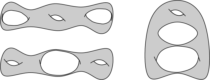
Figure 6: Three degenerations of a Klein surface $\Sigma$ of type $(2,0)_{k}$, viewed from the covering symmetric Riemann surface, of genus $\hat{g}=3$. Upper left: $\Sigma$ degenerates to a Klein bottle via pinching of a handle. Lower left: $\Sigma$ degenerates to a torus via pinching of a Klein handle. Right: $\Sigma$ degenerates to a Klein bottle via pinching of a Klein handle.

Note that unstable “tadpole” degenerations involving single disks or crosscaps with just one closed string insertion are excluded from the above formulas. To make sense of these degenerations, we note that the corresponding singular Riemann surfaces always arise as the common limit of two worldsheets of different topology. Namely, a real node of the covering surface can be smoothed to yield either a disk or a crosscap in the quotient. This is a principle that we have encountered in our A-model discussions in section 3. By adding the two contributions, we obtain the insertion of a tadpole state on the limiting Riemann surface. Explicitly,

$$\begin{split}\partial_{\bar{i}}\bigl{(}{{\cal F}}^{(g,h)}+{{\cal R}}^{(g,h-1)}\bigr{)}&\underset{\rm tadpole}{\supset}-\sqrt{2}\Delta_{\bar{i}}^{j}{{\cal F}}^{(g,h-1)}_{j}\\ \partial_{\bar{i}}\bigl{(}{{\cal K}}^{(g,h)}+{{\cal R}}^{(g,h-1)}\bigr{)}&\underset{\rm tadpole}{\supset}-\sqrt{2}\Delta_{\bar{i}}^{j}{{\cal K}}^{(g,h-1)}_{j}\\ \partial_{\bar{i}}\bigl{(}{{\cal K}}^{(g,h)}+{{\cal R}}^{(g-1,h+1)}\bigr{)}&\underset{\rm tadpole}{\supset}-\sqrt{2}\Delta_{\bar{i}}^{j}{{\cal R}}^{(g-1,h)}_{j}\end{split}$$ (4.24)

where the $\sqrt{2}$ again comes from the normalization of the superpotential (4.5).

Let us now assemble these various pieces and consider the holomorphic anomaly for the total topological string amplitudes at order $\chi>0$ in string perturbation theory. As discussed in section 2, these are given by

$${{\cal G}}^{(\chi)}=\frac{1}{2^{\frac{\chi}{2}+1}}\Bigl{[}{\cal F}^{(g_{\chi})}+\sum_{2g+h-2=\chi}{{\cal F}}^{(g,h)}+\sum_{2g+h-1=\chi}{{\cal R}}^{(g,h)}+\sum_{2g+h-2=\chi}{{\cal K}}^{(g,h)}\Bigr{]}$$ (4.25)

By combining the formulas (4.20), (4.22), (4.23), and (4.24), we obtain

$$\partial_{\bar{i}}{{\cal G}}^{(\chi)}=\frac{1}{2}\sum_{\chi_{1}+\chi_{2}=\chi-2}C_{\bar{i}}^{jk}{{\cal G}}^{(\chi_{1})}_{j}{{\cal G}}^{(\chi_{2})}_{k}+\frac{1}{4}\bigl{(}C_{\bar{i}}^{jk}+B_{\bar{i}}^{jk}\bigr{)}{{\cal G}}^{(\chi-2)}_{jk}-\Delta_{\bar{i}}^{j}{{\cal G}}^{(\chi-1)}_{j}$$ (4.26)

It is a pleasant surprise that this final form of the holomorphic anomaly equation is very similar to the extended holomorphic anomaly of [8], see (4.20). Note that the prefactor in the second term

$${C^{P}}_{\bar{i}}^{jk}=\frac{1}{2}\bigl{(}C_{\bar{i}}^{jk}+B_{\bar{i}}^{jk}\bigr{)}=C_{\bar{i}}^{jl}\;\frac{\delta_{l}^{k}+P_{l}^{k}}{2}$$ (4.27)

is simply the projection of the Yukawa coupling onto the parity-invariant states. Moreover, we note that we may also endow $C_{\bar{i}}^{jk}$ in the first term of (4.26) with the same projector (4.27). This is because the one-point functions ${{\cal G}}^{(\chi)}_{j}$ with insertion of a parity-odd field must vanish identically. (The two-point function ${{\cal G}}^{(\chi)}_{jk}$ might not vanish when both fields are odd, so here we must use that the projector comes out of the degeneration of Riemann surfaces.) Finally, we can also insert a projector in front of the last term in (4.26),

$${\Delta^{P}}_{\bar{i}}^{j}=\Delta_{\bar{i}}^{l}\;\frac{\delta_{l}^{j}+P_{l}^{j}}{2}$$ (4.28)

to obtain

$$\partial_{\bar{i}}{{\cal G}}^{(\chi)}=\frac{1}{2}\sum_{\chi_{1}+\chi_{2}=\chi-2}{C^{P}}_{\bar{i}}^{jk}{{\cal G}}^{(\chi_{1})}_{j}{{\cal G}}^{(\chi_{2})}_{k}+\frac{1}{2}{C^{P}}_{\bar{i}}^{jk}{{\cal G}}^{(\chi-2)}_{jk}-{\Delta^{P}}_{\bar{i}}^{j}{{\cal G}}^{(\chi-1)}_{j}$$ (4.29)

This holomorphic anomaly equation is even closer to (4.20), with the important difference that fields that are projected out by the orientifold have completely decoupled, as we should have expected.

As is well-known, parity defines a holomorphic involution

$$P:M\to M$$ (4.30)

of the moduli space of the topological string, and the invariant subspace,

$$M^{P}=\{P(m)=m\}\subset M$$ (4.31)

is the moduli space of the orientifold.

As a consequence of these observations, all the results on solving the holomorphic anomaly equation by Feynman diagrams [2, 8, 12, 19], and on the polynomial structure of the solutions [61, 14, 15] will carry over with no essential modification to the orientifold situation. In particular, since $M^{P}$ is a special Kähler submanifold of the special Kähler manifold $M$, the special geometry relation

$${{R_{{\bar{i}}j}}^{k}}_{l}=C_{{\bar{i}}}^{mk}C_{jml}-G_{{\bar{i}}j}\delta^{k}_{l}-G_{{\bar{i}}l}\delta^{k}_{j}$$ (4.32)

will continue to hold on the orientifold moduli space, and allow for the construction of propagators, terminators, etc.. In the examples below, we will however only deal with one-parameter models, with $M^{P}=M$, so we would have little use for developing this general formalism explicitly.

A notable difference to the works [12, 19] is that (4.29) is an equation only for the total topological amplitude (4.25), and not for the ${{\cal F}}^{(g,h)}$, etc., individually. Namely, tadpole cancellation does not allow introducing a free ’t Hooft parameter into (2.10), in addition to the string coupling. Nevertheless, we can still compute individual amplitudes ${{\cal F}}^{(g,h)}$ for fixed $h$ if we restrict to dependence on the discrete open string moduli, as was done in [8]. This can be seen as a replacement for inserting continuous open string moduli on the worldsheet boundaries, which we have argued before generically decouple from the topological amplitudes.

5 The Examples in the B-model

The topological B-model is governed at closed string tree-level by special geometry, which coincides for Calabi-Yau threefolds with the mathematical theory of variation of Hodge structure [62]. The workhorse [47] is the Picard-Fuchs differential equation satisfied by the periods of the holomorphic three-form. By extension, the open string tree-level information (domainwall tensions) can also be obtained by solving an appropriate differential equation [63], which in the absence of open string moduli is simply an inhomogeneous version of the Picard-Fuchs equation [29, 43]. This might be referred to as ${\cal N}=1$ special geometry, and is related to the mathematical theory of Poincaré normal functions.

The extension to orientifold backgrounds is rather straightforward. As explained in section 4, the tree level data now consists of the full superpotential, and when tadpoles are canceled still fits into the framework of normal functions.

Loop amplitudes can be computed by solving the holomorphic anomaly equations, for which there are several well-known techniques. The holomorphic ambiguities can be fixed by imposing appropriate boundary conditions at the various singular loci in moduli space. One of the outcomes of our computations in this section is that the holomorphic ambiguities for open and unoriented string amplitudes appear to be often simpler than their closed string counterparts.

5.1 Tree-level data

Recall that our three examples were defined in the A-model as the quintic in ${\mathbb{P}}^{4}$, the bicubic in ${\mathbb{P}}^{5}$, and the total bundle of the canonical bundle over ${\mathbb{P}}^{2}$ (local ${\mathbb{P}}^{2}$). The involution defining the orientifold came in each case from the standard complex conjugation of the corresponding projective space. The D-branes are wrapped on the fixed locus of this involution, and to cancel the tadpoles we need exactly one D-brane in the covering space. In each case, there are two brane vacua, and the topological string amplitudes depend on the discrete parameter $\epsilon=\pm 1$ in addition to the bulk Kähler parameter $t$.

The mirror of the quintic is the mirror quintic, which can be obtained by blowing up singularities of an appropriate orbifold of a one-parameter family of quintics. The Picard-Fuchs operator is

$${\cal L}=\theta^{4}-5z(5\theta+1)(5\theta+2)(5\theta+3)(5\theta+4)$$ (5.1)

Where $\theta=zd/dz$, and $z$ is the complex structure parameter of the mirror family, which is related to the Kähler parameter of the quintic by the mirror map,

$$t(z)=\frac{\varpi_{1}(z)}{\varpi_{0}(z)}$$ (5.2)

Here $\varpi_{0}(z)$ and $\varpi_{1}(z)$ are the analytic and first logarithmic solutions, respectively, of the Picard-Fuchs differential equation

$${\cal L}\varpi(z)=0$$ (5.3)

around $z=0$.

The mirror of the two brane vacua on the real quintic is a certain pair of matrix factorizations of the Landau-Ginzburg superpotential [64]. The corresponding normal function is studied in detail in [43]. It can be represented as the difference of curves $[C_{+}-C_{-}]\in{\rm CH}^{2}(Y)$, where

$$\begin{split}C_{\pm}=\{x_{1}+x_{2}=0,\;&x_{3}+x_{4}=0,x_{5}^{2}\pm\sqrt{5\psi}x_{1}x_{3}=0\}\\ &\subset Y=\{x_{1}^{5}+x_{2}^{5}+x_{3}^{5}+x_{4}^{5}+x_{5}^{5}-5\psi x_{1}x_{2}x_{3}x_{4}x_{5}=0\}\end{split}$$ (5.4)

($z=(5\psi)^{-5}$). The domainwall tension ${\cal T}=\int_{\Gamma}\Omega$ (with $\partial\Gamma=C_{+}-C_{-}$) satisfies the inhomogeneous Picard-Fuchs equation

$${\cal L}{\cal T}(z)=c\sqrt{z}$$ (5.5)

where $c=\frac{15}{16\pi^{2}}$.

The mirror of the orientifold action on $X$ is just the trivial involution on $Y$ [41], acting on D-branes by duality. In other words, the superstring version would simply be the type I string compactified on $Y$. This means that topologically, the O-plane charge can be expressed in terms of the tangent bundle of the mirror quintic

$${\rm ch}(\text{O-plane})\propto\sqrt{L(\textstyle{\frac{1}{4}}TY)}$$ (5.6)

As we have mentioned in section 2, it is not clear in general how the orientifold plane is represented holomorphically. However, in the context of type I on the quintic, we have the more elementary expression (4.1) for the superpotential [58], which can be reduced to the statement that (5.6) is also valid holomorphically. Since by the adjunction formula, the Chern classes of the quintic come from projective space, they are independent of the complex structure parameter $z$. (Although we have not checked this explicitly, we expect that the orbifold by $({\mathbb{Z}}_{5})^{3}$ will not affect this conclusion, and at most contribute an overall normalization factor, rather as in [43].) As a consequence, the superpotential ${\cal W}$, see eq. (4.5), satisfies the same differential equation (5.5), with $c\to{\it i}c/2$, where we have inserted a factor of ${\it i}$ for consistency with previous work, and we have removed the factor of $\sqrt{2}$ from ${\cal W}$ because this is more convenient when working with the normalization (2.12) for the topological string amplitudes. As normalization benchmark, we give here the expansion of the normalized Yukawa coupling and normalized infinitesimal invariant in terms of $q=\exp(2\pi{\it i}t)$

$$\begin{split}C_{ttt}&=5+2875q+4876875q^{2}+\cdots\\ -{\it i}\Delta_{tt}&=\frac{15}{2}q^{1/2}+3450q^{3/2}+6801570q^{5/2}+\cdots\end{split}$$ (5.7)

and turn to the other examples.

The mirror of the bicubic was studied in [66]. The Picard-Fuchs operator is

$${\cal L}=\theta^{4}-9z(3\theta+1)^{2}(3\theta+2)^{2}$$ (5.8)

The mirror of the real bicubic as orientifold and D-brane has not been studied in detail yet. It should not be hard to obtain the explicit representatives of the normal function, however we will not really need this for the computational purposes in this section. It suffices to note that the inhomogeneous Picard-Fuchs equation governing the tree level data is

$${\cal L}{\cal W}(z)=\frac{9{\it i}}{32\pi^{2}}\sqrt{z}$$ (5.9)

The normalization factor can be checked by computing the first term in the Gromov-Witten expansion of the (normalized) superpotential

$$-4\pi^{2}{\it i}\frac{{\cal W}(z(q))}{\varpi_{0}(z)}=\sum_{d\;{\rm odd}}\tilde{n}^{(0,1)}_{d}q^{d/2}=2\sum_{\genfrac{}{}{0.0pt}{2}{\scriptstyle d\;{\rm odd}}{\scriptstyle k\;{\rm odd}}}\frac{1}{k^{2}}n^{(0,{\rm real})}_{d}q^{dk/2}$$ (5.10)

in the A-model. In fact, it has been shown [65] that the theorems of [30] also hold for the bicubic, i.e., (5.10) is valid rigorously to all orders. The second step in (5.10) is the BPS expansion and the $n^{(0,{\rm real})}_{d}$ are (conjecturally) all integer.

The mirror of local ${\mathbb{P}}^{2}$ is captured, see e.g., [57], by the family of elliptic curves with equation

$$x_{1}^{3}+x_{2}^{3}+x_{3}^{3}-3\psi x_{1}x_{2}x_{3}=0$$ (5.11)

where the $x_{i}$ are viewed as ${\mathbb{C}}^{*}$-variables. The Picard-Fuchs operator is

$${\cal L}=\theta^{3}-3z\theta(3\theta+1)(3\theta+2)$$ (5.12)

(Where, similarly to as before $z=(3\psi)^{-3}$, and $\theta=zd/dz$.) To obtain the inhomogeneous version, we can take the same shortcut as for the bicubic. The extension reads

$${\cal L}{\cal W}(z)=-\frac{{\it i}}{16\pi^{2}}\sqrt{z}$$ (5.13)

In fact, it is not hard to check that the corresponding normal function can be represented by the two points on the Riemann surface (5.11)

$$p_{\pm}=\{x_{1}+x_{2}=0,x_{3}=\pm\sqrt{3\psi}x_{1}\}\subset\{x_{1}^{3}+x_{2}^{3}+x_{3}^{3}-3\psi x_{1}x_{2}x_{3}=0\}$$ (5.14)

Namely, we can write the domainwall tension between brane vacua as

$${\cal T}=\int_{p_{+}}^{p_{-}}\lambda$$ (5.15)

where $\lambda\propto\log(x_{2}/x_{3})dx_{1}/x_{1}$ is the reduction of the holomorphic three-form to the curve.

An alternative way to obtain the inhomogeneous term in the Picard-Fuchs equation is to study carefully the monodromy properties of the domainwall tension/superpotential as an analytic function over the entire (thrice-punctured) $z$-plane. This was done for the quintic in [29]. The order-two branch points at $z=0$ and $z=\infty$ are easily identified, and the prefactor $c$ follows from requiring integrality of the monodromy matrices around the conifold. This exercise could be repeated for the bicubic and local ${\mathbb{P}}^{2}$, but we will omit this here.

We conclude this subsection by giving the explicit results for the genus $0$ real enumerative invariants for the three models discussed above in table 5.

$d$	quintic	bicubic	local ${\mathbb{P}}^{2}$
1	15	9	$-1$
3	765	90	$1$
5	544125	15759	$-5$
7	487998390	3297987	$42$
9	536543881350	841201389	$-429$
11	664513551962205	241496789706	$4939$

Table 5: Genus $0$ real BPS invariants $n^{(0,{\rm real})}_{d}$

5.2 One-loop

The general solution of the holomorphic anomaly of the torus partition function (4.10) is

$${{\cal F}}^{(1)}=\frac{1}{2}\log\Bigl{[}\det G_{{\bar{i}}j}^{-1}{\it e}^{K(3+n-\frac{1}{12}\chi)}|f|^{2}\Bigr{]}$$ (5.16)

where $G_{{\bar{i}}j}$ is the special Kähler metric on moduli space with Kähler potential $K$. The holomorphic ambiguity $f$ can be fixed by imposing the appropriate behavior at the boundaries of moduli space. Of relevance for the one-parameter models are large volume, conifold and orbifold point. In the holomorphic limit, and with above conventions, one obtains

$${{\cal F}}^{(1)}\underset{\rm hol.}{\to}\;\;\frac{1}{2}\log\Bigl{[}\Bigl{(}\frac{q}{z}\frac{dz}{dq}\Bigr{)}\,(\varpi_{0})^{\frac{\chi}{12}-4}z^{-c_{2}/12}{\rm diss}^{-1/6}\Bigr{]}$$ (5.17)

where $c_{2}$ is the second Chern class of the model, and ${\rm diss}=(1-5^{5}z)$, $(1-3^{6}z)$, and $(1-3^{3}z)$ for quintic, bicubic, and local ${\mathbb{P}}^{2}$, respectively.

We now turn to the open/unoriented amplitudes at one-loop. As we have advertised before, only the total amplitude

$$2{{\cal G}}^{(0)}-{{\cal F}}^{(1)}={\cal A}+{\cal M}+{\cal K}$$ (5.18)

($\text{annulus}+\text{M\"{o}bius}+\text{Klein bottle}$) will admit an integral expansion in the sense conjectured in [22]. However, as we have also emphasized, there are also certain individual parts of the amplitude that make sense and can be computed separately. Specifically, by considering pairs of branes/antibranes with discrete Wilson lines $\epsilon_{1},\epsilon_{2}$, it makes sense to isolate a term that depends on these discrete parameters by

$${{\cal G}}^{(0)}(\epsilon_{1},\epsilon_{2})-{{\cal G}}^{(0)}(-\epsilon_{1},\epsilon_{2})-{{\cal G}}^{(0)}(\epsilon_{1},-\epsilon_{2})+{{\cal G}}^{(0)}(-\epsilon_{1},-\epsilon_{2})=4{{\cal F}}^{(0,2)}\epsilon_{1}\epsilon_{2}$$ (5.19)

which is essentially how we define ${{\cal F}}^{(0,2)}$ in our examples.

At the second stage, we compute the amplitude for the Klein bottle, ${\cal K}\equiv{{\cal K}}^{(1,0)}$. (Or more precisely, the amplitude for the Klein bottle plus the $\epsilon$-independent part of the annulus and Möbius amplitude. Note that the Möbius strip does not make any additional contribution in the transverse channel because the tadpole state (or infinitesimal invariant) has no $\epsilon$-independent part.) Finally, we construct the total topological amplitude of our orientifold with one background D-brane. This is of the form

$$2{{\cal G}}^{(0)}(\epsilon)-{{\cal F}}^{(1)}={\cal K}+{{\cal F}}^{(0,2)}\epsilon^{2}={\cal K}+{{\cal F}}^{(0,2)}$$ (5.20)

with no apparent $\epsilon$-dependence.

The solution of the holomorphic anomaly equation of the annulus is for the one-parameter models, and in the holomorphic limit,

$${\cal A}_{t}={{\cal F}}^{(0,2)}_{t}=\frac{1}{2}\Delta_{tt}^{2}C_{ttt}^{-1}+f^{(0,2)}_{t}$$ (5.21)

where $f^{(0,2)}$ is a holomorphic ambiguity. In [8], it was originally claimed that there is an additional term on the RHS. With this additional term, and with a naive ansatz for the BPS expansion of ${{\cal F}}^{(0,2)}$, the holomorphic ambiguity $f^{(0,2)}$ could be fixed such that all expansion coefficients were integer. However, the situation considered in [8] was that of (5.19), so the effective dimension of the gauge group should actually have been zero. The same statement holds in the orientifold setup with exactly one D-brane in the covering space (i.e., $N^{+}=0$ in (4.14)).

In all three examples that we study, we find that the low degree Gromov-Witten invariants $\tilde{n}^{(0,2)}_{d}$ of table 1 are reproduced by (5.21) with $f^{(0,2)}\equiv 0$. This pattern persists for all genus $0$ amplitudes with an arbitrary number of boundaries, to which we will return below. The precise way is

$${{\cal F}}^{(0,2)}=\sum_{d\;{\rm even}}\tilde{n}^{(0,2)}_{d}q^{d/2}$$ (5.22)

The Klein bottle contribution (4.12) to the holomorphic anomaly of ${{\cal G}}^{(0)}$ can be integrated by the same procedure as that leading to (5.16). We first note that when the orientifold projection acts trivially on the moduli space, we have

$$\partial_{\bar{i}}\partial_{j}{\cal K}=\frac{1}{2}{\rm Tr}\bigl{[}C_{\bar{i}}C_{j}P\bigr{]}=\frac{1}{2}C_{jkl}C_{\bar{i}}^{kl}-G_{{\bar{i}}j}$$ (5.23)

This can be seen by using that with respect to the convenient $tt^{*}$-basis for the Ramond-Ramond ground states, the chiral ring multiplication matrices take the form

$$C_{i}=\begin{pmatrix}0&0&0&0\\ \delta_{i}^{l}&0&0&0\\ 0&C_{im}^{\;\;\;\;{\bar{l}}}&0&0\\ 0&0&G_{i{\bar{m}}}&0\end{pmatrix}\,,\qquad C_{\bar{j}}=\begin{pmatrix}0&G_{{\bar{j}}m}&0&0\\ 0&0&C_{{\bar{j}}{\bar{m}}}^{\;\;\;\;l}&0\\ 0&0&0&\delta_{{\bar{j}}}^{\bar{l}}\\ 0&0&0&0\end{pmatrix}$$ (5.24)

and $P$ is represented by (2.3). In turn, (5.23) can be integrated by using the special geometry relation for the Ricci tensor, (4.32). This yields

$${\cal K}=\frac{1}{2}\log\bigl{(}\det G_{{\bar{i}}j}^{-1}{\it e}^{K(n-1)}|f^{(1,0)_{k}}|^{2}\bigr{)}$$ (5.25)

We can fix the holomorphic ambiguity of the Klein bottle by expanding ${\cal K}$ around $q=0$ in the holomorphic limit and compare with the localization results of section 3.

$${\cal K}\underset{\rm hol.}{\to}\sum_{d\;{\rm even}}\tilde{n}^{(1,0)_{k}}_{d}q^{d/2}$$ (5.26)

It turns out that in all three cases, the holomorphic limit can be written as

$${\cal K}\to-\frac{1}{2}\log\Bigl{[}\Bigl{(}\frac{q}{z}\frac{dz}{dq}\Bigr{)}{\rm diss}^{-1/4}\Bigr{]}$$ (5.27)

where ${\rm diss}=0$ describes the conifold locus in moduli space (see above). We see that as for the torus amplitude, the Klein bottle exhibits a universal singular behavior associated with the conifold. It will not be hard, but crucial for future developments, to pinpoint the microscopic origin of this universality.

Finally, we sum annulus and Klein bottle and expand in the holomorphic limit

$${\cal A}+{\cal K}=2\sum_{\genfrac{}{}{0.0pt}{2}{\scriptstyle d\;{\rm even}}{\scriptstyle k\;{\rm odd}}}\frac{1}{k}n^{(1,{\rm real})}_{d}q^{dk/2}$$ (5.28)

to extract the real BPS invariants $n^{(1,{\rm real})}_{d}$. We have checked integrality up to $d\sim 50$, and list the first few in table 6.

$d$	quintic	bicubic	local ${\mathbb{P}}^{2}$
2	$0$	0	0
4	$17725$	$693$	$3$
6	$36079420$	$381912$	$-44$
8	$65378348025$	$167597505$	$675$
10	$116755627418596$	$70912518192$	$-10596$
12	$209184366237053675$	$29843206833573$	$169815$

Table 6: Genus $1$ real BPS invariants $n^{(1,{\rm real})}_{d}$

5.3 Next loop

At the next order in perturbation theory, $\chi=1$, there are three non-trivial worldsheets contributing to the total amplitude. (In our examples, all amplitudes ${{\cal R}}^{(g,h)}$ with an odd number of crosscaps vanish. This follows from the vanishing of the crosscap contribution to the superpotential, discussed around eq. (5.6), together with the recursive nature of the holomorphic anomaly equations. In the A-model, the vanishing of the ${{\cal R}}^{(g,h)}$ is a consequence of local tadpole cancellation, as discussed on page 3.) Consider

$$2{{\cal G}}^{(1)}={{\cal F}}^{(0,3)}+{{\cal F}}^{(1,1)}+{{\cal K}}^{(1,1)}$$ (5.29)

The solution of the holomorphic anomaly equation for ${{\cal F}}^{(0,3)}$ is

$$\begin{split}{{\cal F}}^{(0,3)}&=-{{\cal F}}^{(0,2)}_{j}\Delta^{j}-\frac{1}{2}\Delta_{jk}\Delta^{j}\Delta^{k}-\frac{1}{6}C_{jkl}\Delta^{j}\Delta^{k}\Delta^{l}+{\it hol.\ amb.}\\ &=-{{\cal F}}^{(0,2)}_{t}\Delta^{t}-\frac{1}{3}\Delta_{tt}\Delta^{t}\Delta^{t}\end{split}$$ (5.30)

where in the second line we have specialized to the one-parameter models. Again, it turns out that the localization results are reproduced exactly by (5.30) with vanishing holomorphic ambiguity $f^{(0,3)}=0$.

The oriented one-loop amplitude with one boundary is given by

$$\begin{split}{{\cal F}}^{(1,1)}&=\frac{1}{2}S^{jk}\Delta_{jk}-{{\cal F}}^{(1,0)}_{j}\Delta^{j}+\frac{1}{2}C_{jkl}S^{kl}\Delta^{j}-\Bigl{(}{\frac{\chi}{24}}-1\Bigr{)}\Delta+{\it hol.amb.}\\ &=-{{\cal F}}^{(1,0)}_{t}\Delta^{t}-\Bigl{(}\frac{\chi}{24}-1\Bigr{)}\Delta+f^{(1,1)}\end{split}$$ (5.31)

(As usual, the term with $\chi/24$ is absent for local ${\mathbb{P}}^{2}$ for appropriate choice of terminator.) For the quintic and bicubic, we have no localization results to fix the holomorphic ambiguity. For local ${\mathbb{P}}^{2}$, we obtain in the above conventions

$$f^{(1,1)}=\frac{{\it i}}{24}(-z)^{1/2}$$ (5.32)

There is one non-orientable diagram that contributes to the amplitude at $\chi=1$. Its holomorphic anomaly equation is solved by

$$\begin{split}\partial_{\bar{i}}{{\cal K}}^{(1,1)}&=\frac{1}{2}{C^{P}}_{\bar{i}}^{jk}\Delta_{jk}-{\cal K}_{j}\Delta_{\bar{i}}^{j}\\ &=\partial_{\bar{i}}\bigl{(}\frac{1}{2}{S^{P}}^{jk}\Delta_{jk}-{\cal K}_{j}\Delta^{j}\bigr{)}+\frac{1}{2}{S^{P}}^{jk}C_{jkl}\Delta^{l}_{\bar{i}}+\Bigl{(}\frac{1}{2}C_{jkl}{C^{P}}_{\bar{i}}^{kl}-G_{{\bar{i}}j}\Bigr{)}\Delta^{j}\\ &=\partial_{\bar{i}}\bigl{(}\frac{1}{2}{S^{P}}^{jk}\Delta_{jk}-{\cal K}_{j}\Delta^{j}+\frac{1}{2}C_{jkl}{S^{P}}^{kl}\Delta^{j}-\Delta\bigr{)}\end{split}$$ (5.33)

where $C^{P}_{ijk}=C_{ijl}P^{l}_{k}$, cf.., (2.2). Specializing to our one-parameter models, we obtain

$${{\cal K}}^{(1,1)}=-{\cal K}_{t}\Delta^{t}-\Delta+f^{(1,1)_{k}}$$ (5.34)

For local ${\mathbb{P}}^{2}$, we find that we reproduce the localization results of table 2 for $f^{(1,1)_{k}}=0$. For the quintic and the bicubic, we find that the localization results are also reproduced, but in fact by the first term, $-{\cal K}_{t}\Delta^{t}$ in (5.34) alone. We interpret this to say that since there is no observable that would distinguish between ${{\cal F}}^{(1,1)}$ and ${{\cal K}}^{(1,1)}$, only the sum ${{\cal F}}^{(1,1)}+{{\cal K}}^{(1,1)}$ can have a truly invariant meaning. (In the A-model, this mixing is possibly related to our generous treatment of real torus fixed points.) Consequently, we attempt to fix the holomorphic ambiguity only for the combination

$${{\cal F}}^{(1,1)}+{{\cal K}}^{(1,1)}=-{{\cal F}}^{(1,0)}_{t}\Delta^{t}-{\cal K}_{t}\Delta^{t}-\frac{\chi}{24}\Delta+f^{(1,1)}\,,$$ (5.35)

by requiring vanishing of the integral invariants in low degree. We find for the quintic

$$f^{(1,1)}=\frac{85}{8}{\it i}\varpi_{0}(z)\sqrt{z}$$ (5.36)

and for the bicubic,

$$f^{(1,1)}=\frac{27}{8}{\it i}\varpi_{0}(z)\sqrt{z}$$ (5.37)

The expansion

$${\it i}({{\cal F}}^{(0,3)}+{{\cal F}}^{(1,1)}+{{\cal K}}^{(1,1)})=2\sum_{\genfrac{}{}{0.0pt}{2}{\scriptstyle d\;{\rm odd}}{\scriptstyle k\;{\rm odd}}}\bigl{(}n^{(2,{\rm real})}_{d}-\frac{1}{24}n^{(0,{\rm real})}_{d}\bigr{)}q^{kd/2}$$ (5.38)

with $n^{(0,{\rm real})}_{d}$ taken from (5.10) then delivers the integers shown in table 7.

$d$	quintic	bicubic	local ${\mathbb{P}}^{2}$
1	$0$	0	0
3	$0$	$0$	$0$
5	$-55640$	$-693$	$-10$
7	$-159440655$	$-568557$	$229$
9	$-387012696805$	$-328426623$	$-4833$
11	$-878665820903170$	$-175272593346$	$96823$

Table 7: Genus $\hat{g}=2$ real BPS invariants $n^{(2,{\rm real})}_{d}$

5.4 Further checks

Let us first digress a bit on the systematics of the BPS expansion that we have been using. We recall that we are working in the normalization (2.12) for the total topological amplitude,

$${{\cal G}}^{(\chi)}=\frac{1}{2}\Bigl{[}{{\cal F}}^{(g_{\chi})}+\sum{{\cal F}}^{(g,h)}+\sum{{\cal K}}^{(g,h)}\Bigr{]}$$ (5.39)

(where $g_{\chi}\equiv\frac{\chi}{2}+1$). According to [21], the purely closed string contribution to this sum admits a large volume expansion of the form

$$\sum_{g}\tilde{\lambda}^{2g-2}{{\cal F}}^{(g)}(t)=\sum_{g,d,k}n^{(g)}_{d}\,\frac{1}{k}\Bigl{(}2\sin\frac{\tilde{\lambda}k}{2}\Bigr{)}^{2g-2}\,q^{kd}$$ (5.40)

in which all $n^{(g)}_{d}$ (Gopakumar-Vafa invariants) are integer. Our computations in the previous subsections indicate that the rest of the amplitude should be expanded as

$$\sum_{\chi}\lambda^{\chi}{\it i}^{\chi}\Bigl{(}{{\cal G}}^{(\chi)}-\frac{1}{2}{{\cal F}}^{(g_{\chi})}\Bigr{)}=\sum_{\genfrac{}{}{0.0pt}{2}{\scriptstyle\chi\equiv d\bmod 2}{\scriptstyle k\;{\rm odd}}}n^{(\hat{g},{\rm real})}_{d}\,\frac{1}{k}\Bigl{(}2\sinh\frac{\lambda k}{2}\Bigr{)}^{\chi}\,q^{kd/2}$$ (5.41)

and that the $n^{(\hat{g},{\rm real})}_{d}$ (with $\hat{g}=\chi+1$) should again all be integer. These integers should give an invariant “count” of the number of real curves of genus $\hat{g}$ and degree $d$. (This interpretation is tied to our putting the D-brane on top of the orientifold plane.) Note that the expansions (5.40) and (5.41) can in the future be related by identifying $\tilde{\lambda}={\it i}\lambda$, absorbing the ${\it i}$ into the definition of the topological amplitudes, and redefining the integral invariants by a sign.

Let us now make a few steps in the direction of extending the computations to higher order in perturbation theory. The integration of the holomorphic anomaly equations is straightforward, although the resulting expressions fairly quickly become too lengthy to write down explicitly. Most powerful is the polynomial algorithm of [61], whose extended form is described in [14, 15]. This reduces the problem to finding the right boundary conditions on the amplitudes in order to fix the holomorphic ambiguity. A lot of progress has recently been made on this problem, including in the compact case [67]. It seems likely that a more detailed analysis of the results in the present paper will allow a better understanding of the boundary conditions also in the extended case. For the time being, we will extract what we can from our localization results in the A-model, and then present a few checks of the enumerative aspects of the $n^{(\hat{g},{\rm real})}_{d}$.

The amplitude at order $\chi=2$ receives contributions from four different worldsheet topologies,

$$2{{\cal G}}^{(2)}-{{\cal F}}^{(2)}={{\cal F}}^{(0,4)}+{{\cal F}}^{(1,2)}+{{\cal K}}^{(1,2)}+{{\cal K}}^{(2,0)}$$ (5.42)

For local ${\mathbb{P}}^{2}$, we have enough A-model data to completely fix the holomorphic ambiguity of the four individual amplitudes, but we will only present the results for the total amplitude, which can be directly computed from the total anomaly equation (4.29). The holomorphic ambiguity is given by

$$\frac{7}{64}z+\frac{7}{288}\frac{1}{(1-27z)}-\frac{9}{128}\frac{1}{(1-27z)^{2}}$$ (5.43)

and the BPS expansion (5.41) then gives the integers in table 8.

$d$	local ${\mathbb{P}}^{2}$
2	0
4	$1$
6	$-63$
8	$2826$
10	$-91309$
12	$2548446$

Table 8: Genus $\hat{g}=3$ real BPS invariants $n^{(3,{\rm real})}_{d}$

We do not have enough data to fix the holomorphic ambiguity of ${{\cal G}}^{(2)}$ for either the quintic or the bicubic. For $\chi=3$, the localization data from table 4 is consistent with the present understanding, and for local ${\mathbb{P}}^{2}$ determines the following integer invariants:

$$n^{(4,{\rm real})}_{1}=0\,,\qquad n^{(4,{\rm real})}_{3}=0\,,\qquad n^{(4,{\rm real})}_{5}=-6\,,\qquad$$ (5.44)

Let us now turn to the checks on the BPS invariants related to their interpretation as enumerating real curves. Consider the complex curves of degree $d$ and genus $\hat{g}$, and let us pretend for simplicity that there is indeed a finite number $n^{(\hat{g})}_{d}$ of them. Complex conjugation acts on this finite set, and we are claiming that the appropriately counted number of fixed points is given by $n^{(\hat{g},{\rm real})}_{d}$. Since all other orbits have order two, we immediately conclude that we must have

$$n_{d}^{(\hat{g},{\rm real})}\equiv n_{d}^{(\hat{g})}\bmod 2$$ (5.45)

We also have the implication

$$n^{(\hat{g})}_{d}=0\Rightarrow n^{(\hat{g},{\rm real})}_{d}=0$$ (5.46)

One can easily check that these constraints are satisfied for all numbers that we have listed in the tables above.

We can also verify a few of the numbers in the above tables directly. In general, we expect that more checks can be done by taking a suitable real section of the computational scheme for Gopakumar-Vafa invariants initiated in [68] and developed in several subsequent works. We also expect a connection with appropriately defined “real Donaldson-Thomas” [69] and “real Pandharipande-Thomas” [70, 71] invariants.

The simplest Gopakumar-Vafa invariants to check are those associated to smooth curves. For local ${\mathbb{P}}^{2}$, these are curves of genus $\hat{g}=\frac{(d-1)(d-2)}{2}$, which are parametrized by a copy of ${\mathbb{C}}{\mathbb{P}}^{\frac{(d+1)(d+2)}{2}-1}$. Their contribution to Gopakumar-Vafa theory is up to a sign simply the Euler characteristic of the projective space,

$$n_{d}^{((d-1)(d-2)/2)}=(-1)^{\frac{d^{2}+3d}{2}}\frac{(d+1)(d+2)}{2}$$ (5.47)

Clearly now, real curves of the same genus and degree are simply parametrized by the corresponding real projective space ${\mathbb{R}}{\mathbb{P}}^{\frac{d^{2}+3d}{2}}$, and it is natural to assume that their contribution will (up to a sign) again be given by the Euler character of the parameter space. The interesting case is when $\frac{d^{2}+3d}{2}$ is even, when the Euler character is $1$. Taking account of the constraint (3.17), we see that when $d\equiv 0$ or $1\bmod 4$, the real invariant should be

$$n^{((d-1)(d-2)/2,{\rm real})}_{d}=\pm 1$$ (5.48)

This leads to a check of $n^{(0,{\rm real})}_{1}=-1$ in table 5 and $n^{(3,{\rm real})}_{4}=1$ in table 8.

We can also interpret $n^{(0,{\rm real})}_{3}$ along those lines. The corresponding complex invariant is according to [68] given by the Euler character of the universal curve ${\cal C}$ over the parameter space ${\mathbb{C}}{\mathbb{P}}^{9}$ of plane cubic curves. ${\cal C}$ is a ${\mathbb{C}}{\mathbb{P}}^{8}$ fibration over ${\mathbb{C}}{\mathbb{P}}^{2}$, and the Euler characteristic is $n^{(0)}_{3}={\bf e}({\cal C})={\bf e}({\mathbb{C}}{\mathbb{P}}^{2})\cdot{\bf e}({\mathbb{C}}{\mathbb{P}}^{8})=27$. In the real version, this simply yields

$$n^{(0,{\rm real})}_{3}={\bf e}({\cal C}^{\rm real})={\bf e}({\mathbb{R}}{\mathbb{P}}^{2})\cdot{\bf e}({\mathbb{R}}{\mathbb{P}}^{8})=1$$ (5.49)

in agreement with table 5 (up to possibly a sign which we shall not attempt to justify).

As a less elementary computation, we can verify the invariants $n^{(1,{\rm real})}_{4}=-n^{(2,{\rm real})}_{5}=693$ on the bicubic. The corresponding complex invariants also coincide, $n^{(1)}_{4}=n^{(2)}_{5}=5520393$, see ref. [67]. This coincidence is similar to $n^{(0)}_{2}=n^{(1)}_{3}=609250$ on the quintic, and can be understood as follows. Let $C_{4}$ be a smooth degree $4$ genus $1$ curve contained in the bicubic. Such a curve spans a unique ${\mathbb{C}}{\mathbb{P}}^{3}\subset{\mathbb{C}}{\mathbb{P}}^{5}$. This ${\mathbb{C}}{\mathbb{P}}^{3}$ meets the bicubic in a degree $9$ curve $C_{9}$, which must be reducible, with one component being $C_{4}$. the other component is a degree $5$ curve $C_{5}$ of genus $2$. Conversely, we can start from $C_{5}$ to obtain $C_{4}$. Thus, $n^{(1)}_{4}=n^{(2)}_{5}$ on the bicubic. The coincidence of the two invariants should be preserved over the reals (again, up to a sign), which is exactly as predicted! But we can in fact do even better.

The BPS invariant $n^{(1)}_{4}=3721431625$ on the quintic was verified in [72]. There are two contributions. The first comes from smooth elliptic quartics in all ${\mathbb{C}}{\mathbb{P}}^{3}$’s inside of ${\mathbb{C}}{\mathbb{P}}^{5}$, and can be computed by localization on the corresponding relative Hilbert scheme. The second contribution comes from plane binodal quartics, and is obtained by a more classical computation. On the bicubic, we have a contribution only from the smooth quartics, because the planes meet the bicubic in too low dimension. (We have used this fact in the previous paragraph.) Thus, $n^{(1)}_{4}=5520393$ on the bicubic is given by a simple localization calculation, and taking a real section of it readily confirms $n^{(1,{\rm real})}_{4}=693$. The invariants $n^{(0,{\rm real})}_{3}$ can be computed in the same manner, as already noted for the quintic in [29].

6 Conclusions

In this paper, we have shown that the extended holomorphic anomaly equation of [8] can also be used to compute topological string amplitudes on Calabi-Yau orientifolds. We have verified that the results match those obtained in the A-model by a computational prescription that can be understood as a real version of the localization formulas on the moduli space of maps. The success of these computations indicates that there is a well-defined underlying Gromov-Witten theory. We have found hints that the correct moduli spaces to define this theory in fact contain domain curves of varying topology, but fixed Euler character. The essential idea is to absorb boundary components that are homologically trivial in the target Lagrangian and shrink to zero size on the domain curve by smoothing the developing real node into a crosscap. For this to make sense in general, the homology class of the Lagrangian wrapped by the D-brane must be equal to that of the fixed point set of the anti-holomorphic involution defining the orientifold (O-plane). We argued that this phenomenon in Gromov-Witten theory should be interpreted physically as a manifestation of a “tadpole cancellation condition” in the topological string.

From the formal point of view, the most interesting result is that the holomorphic anomaly equation for the total amplitude ${{\cal G}}^{(\chi)}$ of the orientifold model simply coincides with the extended holomorphic anomaly equation of [8]. In the A-model, we have obtained a satisfactory BPS interpretation of the total amplitudes, and have verified several of these predictions from the point of view of real enumerative geometry.

Our work leaves several questions unaddressed. Let us mention some of them.
   From the practical point of view, the most immediate problem is to understand the behavior of the orientifold amplitudes at the special points in moduli space other than large volume. The behavior at the conifold should be determined by a simple orientifold version of the usual closed string story [73], and is hence probably also related to orientifolds of $\hat{c}=1$ string at self-dual radius. We expect new effects at the orbifold point due to the “tensionless domainwalls” that appear on the worldvolume of the D-brane, as explained in [29, 8].
   In the physical string, there is an intimate relation between tadpole cancellation and the cancellation of gauge and gravitational anomalies [4]. It seems likely that there should be a similar connection also in the topological string, which it would be interesting to understand this better.
   As a hint in this direction, recall that the oriented one-loop topological amplitudes are expressible in the B-model in terms of holomorphic Ray-Singer torsions for the $\bar{\partial}$-operator coupled to the appropriate vector bundle [2]. Consequently, the non-orientable one-loop amplitudes (Möbius strip and Klein bottle) are certainly related to Ray-Singer torsions twisted by duality, although we have not been able to locate a convenient reference in which such objects are studied. As a consequence of this connection, the one-loop amplitudes generally exhibit a “gravitational anomaly”, i.e., an explicit dependence on the background Kähler metric [74, 75]. For the torus amplitude, this anomaly reduces to a volume-dependent factor when one computes for the Ricci-flat metric on the Calabi-Yau. More generally, the explicit metric dependence can be eliminated by studying appropriate virtual bundles with vanishing topological Chern classes [76], in a way analogous to our tadpole cancellation using anti-branes.
   Also related to the question of anomaly cancellation is the role played by torsion charges, which do figure into tadpole and anomaly cancellation in the physical string. It might be somewhat difficult to come up with a workable example of this in the topological string.
   Perhaps the most intriguing speculation arises in connection with the so-called wavefunction interpretation of the topological string partition function [16]. In [19], it was conjectured that the solutions of the extended holomorphic anomaly equation as one varies the D-brane background should furnish a basis of Witten’s Hilbert space ${\cal H}_{W}$ that arises upon quantization of the symplectic vector space $H^{3}(Y,{\mathbb{R}})$. In the context of orientifolds, it seems very likely that there will only be a finite number of allowed brane configurations satisfying tadpole cancellation. This is suggestive of a distinguished finite-dimensional Hilbert space ${\cal H}_{\rm phys.}$ of physical states inside of ${\cal H}_{W}$, which would be a quite remarkable lesson of the topological string on compact Calabi-Yau manifolds.
   Finally, we can also envisage some applications in the context of string phenomenology. It is well-known that the topological string one-loop amplitudes are related to threshold corrections for gauge and gravitational couplings of an associated superstring compactification on the same Calabi-Yau manifold [77, 2]. The one-loop amplitudes also enter the D-instanton induced superpotentials in type I/II compactifications [78, 79, 80, 81], see [82] for a recent review. The holomorphic anomaly equation should now allow a principled computation of these couplings for a general Calabi-Yau.

Acknowledgments I would like to thank Sergei Gukov, Simeon Hellerman, Sheldon Katz, Hirosi Ooguri, Rahul Pandharipande, Jake Solomon, and Cumrun Vafa for valuable discussions and communications. This work was supported in part by the Roger Dashen Membership at the Institute for Advanced Study and by the NSF under grant number PHY-0503584.

References

- [1] M. Bershadsky, S. Cecotti, H. Ooguri and C. Vafa, “Holomorphic anomalies in topological field theories,” Nucl. Phys. B 405, 279 (1993) [arXiv:hep-th/9302103].
- [2] M. Bershadsky, S. Cecotti, H. Ooguri and C. Vafa, “Kodaira-Spencer theory of gravity and exact results for quantum string amplitudes,” Commun. Math. Phys. 165, 311 (1994) [arXiv:hep-th/9309140].
- [3] M. B. Green and J. H. Schwarz, “Anomaly Cancellation In Supersymmetric D=10 Gauge Theory And Superstring Theory,” Phys. Lett. B 149, 117 (1984).
- [4] J. Polchinski and Y. Cai, “Consistency of Open Superstring Theories,” Nucl. Phys. B 296, 91 (1988).
- [5] D. Friedan, E. J. Martinec and S. H. Shenker, “Conformal Invariance, Supersymmetry And String Theory,” Nucl. Phys. B 271, 93 (1986).
- [6] E. G. Gimon and J. Polchinski, “Consistency Conditions for Orientifolds and D-Manifolds,” Phys. Rev. D 54, 1667 (1996) [arXiv:hep-th/9601038].
- [7] E. Witten, “Topological Sigma Models,” Commun. Math. Phys. 118, 411 (1988).
- [8] J. Walcher, “Extended Holomorphic Anomaly and Loop Amplitudes in Open Topological String,” arXiv:0705.4098 [hep-th].
- [9] M. Marino, “Open string amplitudes and large order behavior in topological string theory,” arXiv:hep-th/0612127.
- [10] B. Eynard, M. Marino and N. Orantin, “Holomorphic anomaly and matrix models,” JHEP 0706, 058 (2007) [arXiv:hep-th/0702110.
- [11] I. Antoniadis, K. S. Narain and T. R. Taylor, “Open string topological amplitudes and gaugino masses,” Nucl. Phys. B 729, 235 (2005) [arXiv:hep-th/0507244].
- [12] P. L. H. Cook, H. Ooguri and J. Yang, “Comments on the Holomorphic Anomaly in Open Topological String Theory,” Phys. Lett. B 653, 335 (2007) [arXiv:0706.0511 [hep-th]].
- [13] G. Bonelli and A. Tanzini, “The holomorphic anomaly for open string moduli,” JHEP 0710, 060 (2007) [arXiv:0708.2627 [hep-th]].
- [14] M. Alim and J. D. Lange, “Polynomial Structure of the (Open) Topological String Partition Function,” JHEP 0710, 045 (2007) [arXiv:0708.2886 [hep-th]].
- [15] Y. Konishi and S. Minabe, “On solutions to Walcher’s extended holomorphic anomaly equation,” arXiv:0708.2898 [math.AG].
- [16] E. Witten, “Quantum background independence in string theory,” arXiv:hep-th/9306122.
- [17] M. Aganagic, R. Dijkgraaf, A. Klemm, M. Marino and C. Vafa, “Topological strings and integrable hierarchies,” Commun. Math. Phys. 261, 451 (2006) [arXiv:hep-th/0312085].
- [18] M. Aganagic, A. Neitzke and C. Vafa, “BPS microstates and the open topological string wave function,” arXiv:hep-th/0504054.
- [19] A. Neitzke and J. Walcher, “Background Independence and the Open Topological String Wavefunction,” arXiv:0709.2390 [hep-th]—.
- [20] H. Ooguri, Y. Oz and Z. Yin, “D-branes on Calabi-Yau spaces and their mirrors,” Nucl. Phys. B 477, 407 (1996) [arXiv:hep-th/9606112].
- [21] R. Gopakumar and C. Vafa, “M-theory and topological strings. I, II,” arXiv:hep-th/9809187, arXiv:hep-th/9812127.
- [22] H. Ooguri and C. Vafa, “Knot invariants and topological strings,” Nucl. Phys. B 577, 419 (2000) [arXiv:hep-th/9912123].
- [23] M. Kontsevich, “Enumeration Of Rational Curves Via Torus Actions,” arXiv:hep-th/9405035.
- [24] S. H. Katz and C. C. Liu, “Enumerative Geometry of Stable Maps with Lagrangian Boundary Conditions and Multiple Covers of the Disc,” Adv. Theor. Math. Phys. 5, 1 (2002) [arXiv:math.ag/0103074].
- [25] T. Graber and E. Zaslow, “Open string Gromov-Witten invariants: Calculations and a mirror ’theorem’,” arXiv:hep-th/0109075.
- [26] P. Mayr, “Summing up open string instantons and N = 1 string amplitudes,” arXiv:hep-th/0203237.
- [27] D. E. Diaconescu, B. Florea and A. Misra, “Orientifolds, unoriented instantons and localization,” JHEP 0307, 041 (2003) [arXiv:hep-th/0305021].
- [28] V. Bouchard, B. Florea and M. Marino, “Counting higher genus curves with crosscaps in Calabi-Yau orientifolds,” JHEP 0412, 035 (2004) [arXiv:hep-th/0405083].
- [29] J. Walcher, “Opening Mirror Symmetry on the Quintic,” Comm. Math. Phys. 276 671-689 (2007) [arXiv:hep-th/0605162]
- [30] R. Pandharipande, J. Solomon and J. Walcher, “Disk enumeration on the Quintic 3-fold,” arXiv:math/0610901
- [31] J. M. F. Labastida, M. Marino and C. Vafa, “Knots, links and branes at large N,” JHEP 0011, 007 (2000) [arXiv:hep-th/0010102].
- [32] S. Sinha and C. Vafa, “SO and Sp Chern-Simons at large N,” arXiv:hep-th/0012136.
- [33] B. Acharya, M. Aganagic, K. Hori and C. Vafa, “Orientifolds, mirror symmetry and superpotentials,” arXiv:hep-th/0202208.
- [34] V. Bouchard, B. Florea and M. Marino, “Topological open string amplitudes on orientifolds,” JHEP 0502, 002 (2005) [arXiv:hep-th/0411227].
- [35] B. Eynard and N. Orantin, “Invariants of algebraic curves and topological expansion,” arXiv:math-ph/0702045.
- [36] V. Bouchard, A. Klemm, M. Marino and S. Pasquetti, “Remodeling the B-model,” arXiv:0709.1453 [hep-th].
- [37] J. Dai, R. G. Leigh and J. Polchinski, “New Connections Between String Theories,” Mod. Phys. Lett. A 4, 2073 (1989).
- [38] P. Horava, “Strings on World Sheet Orbifolds,” Nucl. Phys. B 327, 461 (1989).
- [39] M. Bianchi and A. Sagnotti, “On the systematics of open string theories,” Phys. Lett. B 247, 517 (1990).
- [40] P. Horava, “Equivariant topological sigma models,” Nucl. Phys. B 418, 571 (1994) [arXiv:hep-th/9309124].
- [41] I. Brunner and K. Hori, “Orientifolds and mirror symmetry,” JHEP 0411, 005 (2004) [arXiv:hep-th/0303135].
- [42] K. Hori and J. Walcher, “D-brane categories for orientifolds: The Landau-Ginzburg case,” arXiv:hep-th/0606179.
- [43] D. R. Morrison and J. Walcher, “D-branes and Normal Functions,” arXiv:0709.4028 [hep-th].
- [44] D. E. Diaconescu, A. Garcia-Raboso, R. L. Karp and K. Sinha, “D-brane superpotentials in Calabi-Yau orientifolds.” arXiv:hep-th/0606180.
- [45] G. Weichhold, “Über symmetrische Riemannsche Flächen und die Periodizitätsmodulen der zugehörigen Abelschen Normalintegrale erster Gattung,” Diss. Leipzig. Schlömilch Z. XXVIII. 321-352 (1883).
- [46] P. Buser, M. Seppälä “Real structures of Teichmuüller spaces, Dehn twists, and moduli spaces of real curves,” Math. Z. 232, 547–558 (1999).
- [47] P. Candelas, X. C. De La Ossa, P. S. Green and L. Parkes, “A Pair Of Calabi-Yau Manifolds As An Exactly Soluble Superconformal Theory,” Nucl. Phys. B 359, 21 (1991).
- [48] A. Zinger, “The Reduced Genus-One Gromov-Witten Invariants of Calabi-Yau Hypersurfaces,” arXiv:0705.2397 [math.AG]
- [49] J. P. Solomon “Intersection theory on the moduli space of holomorphic curves with Lagrangian boundary conditions,” arXiv:math.sg/0606429
- [50] C.-C. M. Liu, “Moduli of J-Holomorphic Curves with Lagrangian Boundary Conditions and Open Gromov-Witten Invariants for an -Equivariant Pair,” arXiv:math.sg/0210257
- [51] M. Aganagic and C. Vafa, “Mirror symmetry, D-branes and counting holomorphic discs,” arXiv:hep-th/0012041.
- [52] M. Aganagic, A. Klemm and C. Vafa, “Disk instantons, mirror symmetry and the duality web,” Z. Naturforsch. A 57, 1 (2002) [arXiv:hep-th/0105045].
- [53] I. Brunner, K. Hori, K. Hosomichi and J. Walcher, “Orientifolds of Gepner models,” JHEP 0702, 001 (2007) [arXiv:hep-th/0401137].
- [54] K. Hori, K. Hosomichi, D. C. Page, R. Rabadan and J. Walcher, “Non-perturbative orientifold transitions at the conifold,” JHEP 0510, 026 (2005) [arXiv:hep-th/0506234].
- [55] C. Faber, ”Algorithms for computing intersection numbers on moduli spaces of curves, with an application to the class of the locus of Jacobians,” arXiv:alg-geom/9706006
- [56] T. Graber, R. Pandharipande, “Localization of virtual classes,” Invent. Math. 135 (1999), 487–518, [arXiv:math.ag/9601010]
- [57] A. Klemm and E. Zaslow, “Local mirror symmetry at higher genus,” arXiv:hep-th/9906046
- [58] E. Witten, “New Issues In Manifolds Of SU(3) Holonomy,” Nucl. Phys. B 268, 79 (1986).
- [59] E. Witten, “Chern-Simons Gauge Theory As A String Theory,” Prog. Math. 133, 637 (1995) [arXiv:hep-th/9207094].
- [60] M. R. Douglas and B. Fiol, “D-branes and discrete torsion. II,” JHEP 0509 (2005) 053 [arXiv:hep-th/9903031].
- [61] S. Yamaguchi and S. T. Yau, “Topological string partition functions as polynomials,” JHEP 0407, 047 (2004) [arXiv:hep-th/0406078].
- [62] D. R. Morrison, “Mirror symmetry and rational curves on quintic threefolds: a guide for mathematicians,” J. Amer. Math. Soc. 6 (1993) 223–247, [arXiv:alg-geom/9202004].
- [63] W. Lerche, P. Mayr and N. Warner, “Holomorphic N = 1 special geometry of open-closed type II strings,” arXiv:hep-th/0207259; “N = 1 special geometry, mixed Hodge variations and toric geometry,” arXiv:hep-th/0208039.
- [64] K. Hori and J. Walcher, “D-branes from matrix factorizations,” Talk at Strings ’04, June 28–July 2 2004, Paris. Comptes Rendus Physique 5, 1061 (2004) [arXiv:hep-th/0409204].
- [65] V. Shende, unpublished
- [66] A. Libgober, J. Teitelbaum, “Lines on Calabi-Yau complete intersections, mirror symmetry, and Picard-Fuchs equations,” Internat. Math. Res. Notices 1993, no. 1, 29–39.
- [67] M. x. Huang, A. Klemm and S. Quackenbush, “Topological String Theory on Compact Calabi-Yau: Modularity and Boundary Conditions,” arXiv:hep-th/0612125.
- [68] S. H. Katz, A. Klemm and C. Vafa, “M-theory, topological strings and spinning black holes,” Adv. Theor. Math. Phys. 3, 1445 (1999) [arXiv:hep-th/9910181].
- [69] D. Maulik, N. Nekrasov, A. Okounkov, R. Pandharipande, “Gromov-Witten theory and Donaldson-Thomas theory. I,II,” Compos. Math. 142 (2006), no. 5, 1263–1285, 1286–1304. [arXiv:math.ag/0312059,arXiv:math.ag/0406092]
- [70] R. Pandharipande, R. P. Thomas, “Curve counting via stable pairs in the derived category,” arXiv:0707.2348 [math.AG];
- [71] R. Pandharipande, R. P. Thomas, “Stable pairs and BPS invariants,” arXiv:0711.3899 [math.AG]
- [72] G. Ellingsrud and S. Strømme, “Bott’s formula and enumerative geometry,” J. AMS 9, 175–193 (1996) [arXiv:alg-geom/9411005].
- [73] D. Ghoshal and C. Vafa, “C = 1 String As The Topological Theory Of The Conifold,” Nucl. Phys. B 453, 121 (1995) [arXiv:hep-th/9506122].
- [74] A. Klemm and C. Vafa, unpublished.
- [75] V. Pestun and E. Witten, “The Hitchin functionals and the topological B-model at one loop,” Lett. Math. Phys. 74, 21 (2005) [arXiv:hep-th/0503083].
- [76] I. Biswas and G. Schumacher, “Determinant bundle, Quillen metric, and Petersson-Weil form on moduli spaces,” Geom. Funct. Anal. 9, no. 2, 226–255 (1999)
- [77] I. Antoniadis, E. Gava, K. S. Narain and T. R. Taylor, “Topological amplitudes in string theory,” Nucl. Phys. B 413, 162 (1994) [arXiv:hep-th/9307158].
- [78] R. Blumenhagen, M. Cvetic and T. Weigand, “Spacetime instanton corrections in 4D string vacua - the seesaw mechanism for D-brane models,” Nucl. Phys. B 771, 113 (2007) [arXiv:hep-th/0609191].
- [79] M. Haack, D. Krefl, D. Lust, A. Van Proeyen and M. Zagermann, “Gaugino condensates and D-terms from D7-branes,” JHEP 0701, 078 (2007) [arXiv:hep-th/0609211].
- [80] L. E. Ibanez and A. M. Uranga, JHEP 0703, 052 (2007) [arXiv:hep-th/0609213].
- [81] B. Florea, S. Kachru, J. McGreevy and N. Saulina, “Stringy instantons and quiver gauge theories,” JHEP 0705, 024 (2007) [arXiv:hep-th/0610003].
- [82] N. Akerblom, R. Blumenhagen, D. Lüst, M. Schmidt-Sommerfeld, “D-brane Instantons in 4D Supersymmetric String Vacua,” arXiv:0712.1793 [hep-th]