Analysis of Kelly-optimal portfolios

Abstract

We investigate the use of Kelly’s strategy in the construction of an optimal portfolio of assets. For lognormally distributed asset returns, we derive approximate analytical results for the optimal investment fractions in various settings. We show that when mean returns and volatilities of the assets are small and there is no risk-free asset, the Kelly-optimal portfolio lies on Markowitz Efficient Frontier. Since in the investigated case the Kelly approach forbids short positions and borrowing, often only a small fraction of the available assets is included in the Kelly-optimal portfolio. This phenomenon, that we call condensation, is studied analytically in various model scenarios.

1 Introduction

The construction of an efficient portfolio aims at maximising the investor’s capital, or its return, while minimising the risk of unfavourable events. This problem has been pioneered by Markowitz in [1], where the Mean-Variance (M-V) efficient portfolio has been introduced: it minimizes the portfolio variance for any fixed value of its expected return. Since this rule can be only justified under somewhat unrealistic assumptions (namely a quadratic utility function or a normal distribution of returns, in addition to risk aversion), it should be considered as a first approximation of the optimisation process. Later, several optimisation schemes inspired by Markowitz’s work have been proposed [2, 3, 4]. For a recent thorough overview of the portfolio theory see [5].

A different perspective has been put forward by Kelly in [6], where he shows that the optimal strategy for the long run can be found by maximising the expected value of the logarithm of the wealth after one time step. The optimality of this strategy has long been treated and proven in many different ways [7, 8, 9], according to [10], it was successfully used in real financial markets. For an overview of its continuous time limit see [11]. Recently, the superiority of typical outcomes to average values has been discussed from a different point of view in [12, 13]. Although the Kelly criterion does not employ a utility function, as pointed out by the author himself, a number of economists have adopted the point of view of utility theory to evaluate it [14, 15, 16, 17]. Various modifications, such as fractional Kelly strategies [18] and controlled drawdowns [19], have been proposed to increase security of the resulting portfolios. A thorough review of the advantages, drawbacks and modifications of the Kelly criterion is presented in [20]. For an exposition of the Kelly approach in the context of information theory see [21].

In this paper, we shall discuss the original Kelly strategy in the framework of a simple stochastic model and without assuming the existence of a utility function. We will present approximate analytical results for optimal portfolios in various situations, as well as numerical solutions and computer simulations. We will show that, in the limit of small returns and volatilities, when there is no risk-free asset, the Kelly-optimal portfolio lies on the Efficient Frontier. Furthermore, we shall analytically study the conditions under which diversification is no longer profitable and the optimal portfolio “condensates” on a few assets. Such condensation (or underdiversification) is said to be typical for the Kelly portfolio [20] and here we examine it in various model scenarios. Finally, we will consider the fluctuations of the logarithm of wealth as a measure of risk, and compare it with the classic M-V picture.

This paper is organised as follows. After introducing a multiplicative stochastic model for the dynamics of assets’ prices, we briefly list the main results of the Markowitz Mean-Variance approach. In Sec. 2, we apply Kelly’s method to our model, analysing the case of one, two and many risky assets, both with and without additional constraints. Finally, a combination of the Markowitz Efficient Frontier with the Kelly strategy is investigated. In the appendix we explain the approximations used in this paper as well as a generalisation of the model to the case of correlated asset prices.

1.1 A simple model

We shall study the portfolio optimisation on a very simple model which leads to lognormally distributed returns. Consider $N$ assets, whose prices $p_{i}(t)$ ($i=1,\dots,N$) undergo uncorrelated multiplicative random walks

$$p_{i}(t)=p_{i}(t-1)\,\mathrm{e}^{\eta_{i}(t)}.$$ (1)

Here the random numbers $\eta_{i}(t)$ are drawn from Gaussian density distributions of fixed mean $m_{i}$ and variance $D_{i}$, and are independent of their value at previous time steps. This model can be easily generalised to the case of non-Gaussian densities and correlated price variations as it is discussed in appendix B; the influence of correlations on the Kelly portfolio is investigated in [22]. We assume that the investor knows exact values of the parameters $m_{i},D_{i}$—for the effects of wrong parameter estimates and the details of the Bayesian parameter-learning process see e.g. [23, 20, 24]. We further assume the existence of a risk-free asset paying zero interest rate.

For the sake of simplicity, we do not include dividends, transaction costs and taxes in the model. Hence, the return of asset $i$ is $R_{i}(t):=\left[p_{i}(t)-p_{i}({t-1})\right]/p_{i}({t-1})=\mathrm{e}^{\eta_{i}(t)}-1$ is lognormally distributed with the average $\mu_{i}:=E(R_{i})=\exp[m_{i}+D_{i}/2]-1$ and the volatility $\sigma_{i}^{2}:=E((R_{i}-\mu_{i})^{2})=(\exp[D_{i}]-1)\exp[2m_{i}+D_{i}]$. With $E$ we denote averages over the noise $\eta_{i}(t)$.

A portfolio is determined by the fractions $q_{i}$ of the total capital invested in each one of $N$ available assets; the rest is kept in the risk-free asset. Since $m_{i}$ and $D_{i}$ are fixed, both the Kelly strategy and the Efficient Frontier use one time step optimisation and the basic quantity is the wealth after one time step $W_{1}$. If we set the initial wealth to 1, $W_{1}$ has the form

$$W_{1}=1+\sum_{i=1}^{N}q_{i}R_{i}=1+R_{P},$$ (2)

where $R_{P}:=\sum_{i=1}^{N}q_{i}R_{i}$ is the portfolio return. To simplify the computation we assume infinite divisibility of the investment. Thus, the investment fractions $q_{i}$ are real numbers and do not need to be rounded.

In the portfolio optimisation, some common constraints are often imposed and can as well be applied in the present context. For instance, the non-negativity of the investment fractions $q_{i}\geq 0$ forbids short positions. The condition $\sum_{i=1}^{N}q_{i}=1$ indicates the absence of a riskless asset and $\sum_{i=1}^{N}q_{i}\leq 1$ does not allow the investor to borrow money.

1.2 The Mean-Variance approach

The unconstrained maximisation of the expected capital gain results in the investment of the entire wealth on the asset with the highest expected return; this strategy is sometimes referred to as risk neutral. If the investor has a strong aversion to risk, on the other hand, one might be tempted to simply minimise the portfolio variance $\sigma^{2}_{P}=\sum_{i=0}^{N}q_{i}^{2}\sigma^{2}_{i}$. This leads to invest the entire capital on the risk-free asset with no chance to benefit from asset price movements. The Mean-Variance (MV) approach is much more reasonable as it allows to compromise between the gain and the risk. Here we recount basic results of this standard tool.

With the desired expected return fixed at $E(R_{P})=\mu_{P}$, the constrained minimisation of the portfolio variance $\sigma_{P}^{2}$ is performed using the Lagrange function $\mathcal{L}=E(R_{P}^{2})+\gamma\big{(}E(R_{P})-\mu_{P}\big{)}$ with a Lagrange multiplier $\gamma$. The resulting optimal fractions are

$$\hat{q}_{i}=\mu_{P}\,\frac{\mu_{i}}{C_{2}\sigma_{i}^{2}},\quad\text{where }C_{k}=\sum_{j=1}^{N}\frac{\mu_{j}^{k}}{\sigma_{j}^{2}}.$$ (3)

For $\mu_{P}=0$, $\hat{q}_{i}=0$ for all assets. As we increase $\mu_{P}$, all optimal fractions $\hat{q}_{i}$ grow in a uniform way and their ratios are preserved. At some value $\mu_{P}^{*}$ we reach $\sum\hat{q}_{i}=1$, which means we are investing the entire capital. Any further increase would require to borrow money, with Eq. (3) remaining valid as long as the borrowing rate equals the lending rate (both set to zero here). The relation between $\sigma_{P}$ and $\mu_{P}$ is

$$\sigma_{P}=\mu_{P}/\sqrt{C_{2}}.$$ (4)

This equation is often referred to as Capital Market Line (CML).

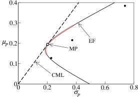
Figure 1: The expected return $\mu_{P}$ versus the standard deviation of the portfolio $\sigma_{P}$. The assets are described by the following parameters: $m_{1}=0.1$, $D_{1}=0.04$, $m_{2}=0.15$, $D_{2}=0.09$, $m_{3}=0.2$, $D_{3}=0.25$ (in the graph they are shown as full circles). The dashed line represents the CML from Eq. (4), the solid line is Efficient Frontier given by Eq. (5), the tangent point of the two is the Market Portfolio. The thick part of EF marks the region where all investment fractions are positive.

If there is no risk-free asset in the market, one has to introduce the additional constraint $\sum_{i=1}^{N}\hat{q}_{i}=1$. It follows that

$$\sigma_{P}^{2}=\frac{C_{0}\mu_{P}^{2}-2C_{1}\mu_{P}+C_{2}}{C_{0}C_{2}-C_{1}^{2}}.$$ (5)

The functional relation between the optimised $\sigma_{P}$ and $\mu_{P}$ is called Efficient Frontier (EF). Since there is only one point on the CML where $\sum_{i}q_{i}=1$, this line is tangent to the EF. The results of this section are plotted in Fig. 1 for a particular choice of three available assets.

2 The Kelly portfolio

When the investor’s capital follows a multiplicative process, after many time steps is its expected value strongly influenced by rare events and in consequence it is not reasonable to form a portfolio by simply maximising $E(W(t))$. The Mean-Variance approach tries to solve this problem in a straightforward, yet criticisable way. We support here the idea that an efficient investment strategy can be found by maximising the investment growth rate in the long run, which is, under the assumption of fixed asset properties, equivalent to maximising the logarithm of the wealth $W_{1}$ after one time step [6]. Thus the key quantity in the construction of a Kelly-optimal portfolio is $v:=E(\ln W_{1})$, the average exponential growth rate of the wealth. We remind that the quantity $\ln W_{1}$ is not a logarithmic utility function.

In [13], $v$ is optimised in a similar context and the authors claim that their procedure corresponds to maximising the median of the distribution of returns. They consider short time intervals and thus small assets returns. Assuming $R_{P}\ll 1$ (very small portfolio return), they use the approximation $\ln(1+R_{P})\approx R_{P}-R_{P}^{2}/2$ of the logarithm in the expression of $v$ before maximising it. However, while such an expansion is only justified for $R_{P}\ll 1$, the maximum of the resulting function is at $R_{P}=1$, in contradiction with the hypothesis. We will develop a different approximation in the following.

First, the unconstrained maximisation of $v$ is achieved by solving the set of equations $\partial v/\partial q_{i}=0$ ($i=1,\dots,N$). After exchanging the order of the derivative and the average, we obtain the condition

$$E\bigg{(}\frac{R_{i}}{1+\sum_{j}q_{j}R_{j}}\bigg{)}=0\qquad(i=1,\dots,N).$$ (6)

In our case, $R_{i}$ has a lognormal distribution and to our knowledge, this set of equations cannot be solved analytically. With the help of the approximations introduced in the appendix we shall work out approximative solutions for some particular cases. We emphasize an important restriction which applies to all solutions of Eq. (6). Since returns $R_{i}$ lie in the range $(-1,\infty)$, when $\sum_{i=1}^{N}q_{i}>1$ or when there is an investment fraction $q_{i}<0$, there is a nonzero probability that $W_{1}$ is negative and hence $v=E(\ln W_{1})$ is not well defined. Since Kelly’s approach focuses on the long run, it requires strictly zero probability of getting bankrupted in one turn. As a consequence, for lognormally distributed returns any Kelly strategy must obey $q_{i}\geq 0$ and $\sum_{i=1}^{N}q_{i}\leq 1$, i.e. both short selling and borrowing must be avoided.

2.1 One risky asset

Let us begin the reasoning with the case of one risky asset. We want to find the optimal investment fraction $q$ of the available wealth. The remaining fraction $1-q$ we keep in cash at the risk-free interest rate which, without loss of generality, is set to zero. This problem is described by Eq. (6) in one dimension; even this simplest case has no analytical solution. Nevertheless, for a given $D$, one can ask what is the value $m_{<}$ for which it becomes profitable to invest a positive fraction of the investor’s capital in the risky asset. This can be found imposing $q=0$ in Eq. (6), yielding $m_{<}=-D/2$. Similarly, the value $m_{>}$ for which it becomes profitable to invest the entire capital can be found by imposing $q=1$, yielding $m_{>}=D/2$.

We shall look for approximate solutions that are valid for small values of $D$, which is the case treated in appendix A. Using approximation Eq. (20) in Eq. (6) gives

$$\frac{\mathrm{e}^{m}-1}{1-q+q\mathrm{e}^{m}}+\frac{D}{2}\,\frac{\mathrm{e}^{m}(1-q-q\mathrm{e}^{m})}{(1-q+q\mathrm{e}^{m})^{3}}=0.$$

With respect to $q$, this is merely a quadratic equation. Since the solution is rather long, we first simplify the equation using $m,D\ll 1$ as in Eq. (21), leading to the result

$$\hat{q}=\frac{1}{2}+\frac{m}{D}.$$ (7)

Since borrowing and short selling are forbidden, for $m<-D/2$ is $\hat{q}=0$ and for $m>D/2$ is $\hat{q}=1$. When asset prices undergo a multiplicative random walk with lognormal returns, both $m$ and $D$ scale linearly with the time scale and hence $\hat{q}$ does not depend on the length of the time step. Notice also that substituting $m=\pm D/2$ gives $\hat{q}=0$ and $\hat{q}=1$, in agreement with the bounds we found before by exact computation. The first order correction to Eq. (7) is $m(4m^{2}-D^{2})/4D^{2}$ which is, for $m\in[-D/2,D/2]$, of order $O(m)$. The validity of the presented approximations can be easily tested by a straightforward numerical maximisation of $E(\ln W_{1})$. As can be seen in Fig. 2, the numerical results are well approximated by the analytical formula Eq. (7) even for $D=1$.

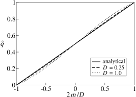
Figure 2: The optimal portfolio fraction $\hat{q}$: a comparison of the analytical result Eq. (7) with a numerical maximisation of $E(\ln W_{1})$.

Notice that, for $m,D\ll 1$, one can approximate $\mu\approx m+D/2$ and $\sigma^{2}\approx D$, which makes the optimal portfolio fraction derived above equal to $\hat{q}^{\prime}=\mu/(\mu^{2}+\sigma^{2})$ obtained in [13]. However, if we check the accuracy of $\hat{q}^{\prime}$, we find a relative error up to 3% for $D=0.01$, and for $D=0.25$ we are already far out of the applicability range with an error around 50%. Also, Eq. (7) is for $m,D\ll 1$ identical to the classical Merton’s result [25] which is derived under the assumption of continuous-time, non-zero consumption of the wealth, and a logarithmic utility function. In [11, 26], the result $\hat{q}=\tfrac{1}{2}+m/D$ is derived for the continuous time limit of our model: $m,D\to 0$, $m/D=\text{const}$.

2.2 Constrained optimisation

The optimal portfolio fractions $q_{i}$ can be derived from Eq. (6) also for $N>1$. Using the same approximations as in the single asset case, we obtain the general formula $\hat{q}_{i}=1/2+m_{i}/D_{i}$ for $i=1,\dots,N$. In our case, Kelly’s approach forbids short selling and hence the assets with $\hat{q}_{i}<0$ do not enter the optimal portfolio. Since borrowing is also forbidden, if $\sum_{i=1}^{N}\hat{q}_{i}>1$, we have to introduce the additional constraint $\sum_{i=1}^{N}q_{i}=1$. This can be done by use of the Lagrange function $\mathcal{L}(\boldsymbol{q},\gamma)=v+\gamma\,\big{(}\sum_{i=1}^{N}q_{i}-1\big{)}$ where $\boldsymbol{q}$ is the vector of investment fractions. The optimal portfolio is then the solution of the set of equations

$$\sum_{j=1}^{N}q_{j}=1,\quad E\bigg{(}\frac{R_{i}}{1+\sum_{i=1}^{N}q_{i}R_{i}}\bigg{)}+\gamma=0\qquad(i=1,\dots,N),$$ (8)

where $R_{i}=\mathrm{e}^{\eta_{i}}-1$. Using the same approximations again, one obtains the general result

$$\hat{q}_{i}=\frac{1}{2}+\frac{m_{i}+\gamma}{D_{i}}.$$ (9)

The Lagrange multiplier $\gamma$ is fixed by the condition $\sum_{j=1}^{N}\hat{q}_{j}=1$. It can occur that even a profitable asset with $m_{i}>-D_{i}/2$ has a negative optimal investment fraction. Since in our case the Kelly approach forbids short selling, this asset has to be eliminated from the optimisation process. In consequence, under some conditions, only a few assets are included in the resulting optimal portfolio. This phenomenon, which we call portfolio condensation, we study closer in sections 2.3 and 2.4. An alternative approach to the constrained Kelly-optimal portfolio is provided by the Kuhn-Tucker equations (see [21]) which, however, can be shown to be equivalent to Eq. (8).

Now we can establish an important link to Markowitz’s approach: in the limit $\mu_{i},\sigma_{i}\to 0$ the Kelly portfolio lies on the constrained Efficient Frontier (no short selling allowed). We shall prove this statement in the following. When all the assets have small $\mu_{i}$ and $\sigma_{i}$, in Eq. (3) and Eq. (5) we can approximate $\mu_{i}\approx m_{i}+D_{i}/2$ and $\sigma_{i}^{2}\approx D_{i}$, leading to the approximative relation for the Efficient Frontier

$$\sigma_{P}^{2}=\frac{\tilde{C}_{0}\mu_{P}^{2}-2\tilde{C}_{1}\mu_{P}+\tilde{C}_{2}}{\tilde{C}_{0}\tilde{C}_{2}-\tilde{C}_{1}^{2}},\quad\text{where }\tilde{C}_{k}=\sum_{j=1}^{N}\frac{(m_{i}+D_{i}/2)^{k}}{D_{i}}.$$ (10)

For the Kelly portfolio we need to work out a similar approximation. Using the condition $\sum_{i}\hat{q}_{i}=1$, for $\gamma$ in Eq. (9) we obtain $\gamma=(1-\tilde{C}_{1})/\tilde{C}_{0}$. In the relations $\mu_{P}=\sum_{i}q_{i}\mu_{i}$ and $\sigma_{P}^{2}=\sum_{i}q_{i}^{2}\sigma_{i}^{2}$ we use the approximations for $\mu_{i},\sigma_{i}$ introduced above. After substituting $q_{i}$ from Eq. (9), for the Kelly optimal portfolio we get

$$\mu_{K}=\frac{\tilde{C}_{0}\tilde{C}_{2}-\tilde{C}_{1}^{2}+\tilde{C}_{1}}{\tilde{C}_{0}},\quad\sigma_{K}^{2}=\frac{\tilde{C}_{0}\tilde{C}_{2}-\tilde{C}_{1}^{2}+1}{\tilde{C}_{0}}.$$ (11)

Both in Eq. (10) and Eq. (11) we consider only the assets that have positive investment fractions. Now it is only a question of simple algebra to show that $\mu_{K}$ and $\sigma_{K}$ given by Eq. (11) fulfill Eq. (10), which completes the proof. Similar, yet weaker, results can be found in the literature. For instance, Markowitz states in [17] that “on the EF there is a point which approximately maximizes $E(\ln W_{1})$.”

Obtained results are illustrated in Fig. 3, where we plot the Efficient Frontier, the constrained Efficient Frontier, and the Kelly portfolio for the same three assets as in Fig. 1. While the original EF is not bounded (for any $\mu_{P}$ exists appropriate $\sigma_{P}$), the constrained EF starts at the point corresponding to the full investment in the least profitable asset and ends at the point corresponding to the most profitable asset. The two lines coincide on a wide range of $\mu_{P}$. In agreement with the previous paragraph, the Kelly portfolio lies close to the constrained EF.

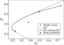
Figure 3: The Efficient Frontier (EF, thin solid line), EF without short selling (bold line), and the Kelly portfolio (solid square) in a particular case of three assets (asset parameters as in Fig. 1).

2.3 Condensation in the two asset case

To illustrate the condensation phenomenon we focus on a simple case here: two risky assets plus a risk-free one, borrowing and short selling forbidden. As we have already seen, without constraints $\hat{q}_{i}=1/2+m_{i}/D_{i}$. Therefore, when $m_{i}<-D_{i}/2$, $\hat{q}_{i}$ is negative and due to forbidden short selling, asset $i$ drops out of the optimal portfolio. In Fig. 4 this threshold is shown for $i=1,2$ by dashed lines. In the lower-left corner (A) we have the region where both assets are unprofitable and the optimal strategy prescribes a fully riskless investment.

When the results of the unconstrained optimisation sum up to one ($\hat{q}_{1}+\hat{q}_{2}=1$), we are advised to invest all our wealth in the risky assets. If both assets are profitable, this occurs when $m_{1}/D_{1}+m_{2}/D_{2}=0$. When only asset $i$ is profitable, we should invest the entire capital on it only when $m_{i}$ equals at least $D_{i}/2$. In Fig. 4 these results are shown as a thick solid curve.

Since borrowing is not allowed, in the region above the solid line constrained optimisation has to be used. The condensation to one of the two assets arises when the optimal fractions $(\hat{q}_{1},\hat{q}_{2})$ are either $(1,0)$ or $(0,1)$; we can find the values $m_{1}^{\prime}$ and $m_{1}^{\prime\prime}$ when this happens. By eliminating $\gamma$ from Eq. (8) and substituting $q_{1}=1$ and $q_{2}=0$ we obtain the condition for the condensation on asset $1$: $E\big{(}(\mathrm{e}^{\eta_{1}}-1)/\mathrm{e}^{\eta_{1}}\big{)}=E\big{(}(\mathrm{e}^{\eta_{2}}-1)/\mathrm{e}^{\eta_{1}}\big{)}$. This can be solved analytically, yielding

$$m_{1}^{\prime}=m_{2}+\frac{D_{1}+D_{2}}{2}.$$ (12)

This equation holds with interchanged indices for the condensation on asset $2$, thus $m_{1}^{\prime\prime}=m_{2}-(D_{1}+D_{2})/2$. Finally, for $m_{1}^{\prime\prime}<m_{1}<m_{1}^{\prime}$ the optimal portfolio contains both assets. The crossover values $m_{1}^{\prime}$ and $m_{2}^{\prime}$ are shown in Fig. 4 as dotted lines. They delimit the region where the portfolio condensates to only one of two profitable assets. A complete “phase diagram” of the optimal investment in the two assets case is presented in Fig. 4 for a particular choice of the assets’ variances. Interestingly, growth-rate optimising strategies have their importance also in evolutionary biology [27] where a similar condensation phenomenon has been observed when studying evolution in an uncertain environment [28].

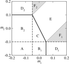
Figure 4: The phase diagram of the two-asset system with $D_{1}=0.1$ and $D_{2}=0.2$. In region A the investor is advised to use only the risk-free asset. In regions B₁, B₂, and C the optimal investment is still partially in the risk-free asset. In regions D₁, D₂, E, F₁, and F₂ one should invest everything in the risky assets. While in regions C and E the investment is divided between the two assets, in shaded regions F₁ and F₂ a nontrivial condensation arises: one is advised to invest all wealth in one asset although the other one is also profitable.

2.4 Many assets with equal volatility

We investigate here the case of an arbitrary large number $N$ of available assets where Kelly’s approach, which forbids borrowing and short selling, gives rise to a portfolio condensation. While the optimal portfolio fractions are given by Eq. (9), to find which assets are included in the optimal portfolio is a hard combinatorial task. To obtain analytical results, we simplify the problem by assuming that the variances of all assets are equal, $D_{i}=D$ ($i=1,\dots,N$). The number of assets contained in the optimal portfolio is labeled as $M$ and the assets are sorted in order of decreasing $m_{i}$ ($m_{1}>m_{2}>\dots>m_{N}$).

If the unconstrained optimisation does not violate forbidden borrowing, then profitability of an asset (i.e., $m_{i}>-D/2$) is the only criterion for including it in the optimal portfolio. When the constrained optimisation is necessary, the optimal portfolio is formed by starting from the most profitable asset $m_{1}$, and adding the others one by one until the last added asset has a nonpositive optimal fraction $q_{M+1}\leq 0$. Summing Eq. (9) from $1$ to $M$, we can write $\gamma$ as $\gamma(M)=D(M^{-1}-1/2)-\tfrac{1}{M}\sum_{1}^{M}m_{i}$. For a given realisation of $\{m_{i}\}$, we can obtain the resulting portfolio size by finding the largest $M$ that satisfies $q_{M}>0$, which leads to

$$m_{M}+\frac{D}{M}>\frac{1}{M}\sum_{i=1}^{M}m_{i}.$$ (13)

This relation tells us how many assets we should invest on, once their expected growths and volatility are known. Notice that for $M=2$ and $D_{1}=D_{2}=D$, this result is consistent with that of Eq. (12) where a special case of the condensation on two assets is described.

Let us follow now a statistical approach. If all $m_{i}$ are drawn from a given distribution $f(m)$, the value of $M$ depends on the current realisation. The characteristic behaviour of the system can be found by taking the average over all possible realizations and replacing $m_{i}$ by $\overline{m}_{i}$. The resulting typical portfolio size $M_{T}$ captures this behaviour and depends on the distribution $f(m)$ and on the number of available assets $N$.

2.4.1 Uniform distribution of $m$

Let us first analyse the case of a uniform distribution of $m_{i}$ within the range $[a,b]$. First we assume that all assets are profitable, i.e. $a+D/2>0$. For $m_{i}$ are sorted in decreasing order, one can show $\overline{m}_{i}=b-(b-a)i/(N+1)$. Since $\overline{m}_{i}$ declines with $i$ linearly, according to Eq. (9) so does $\overline{\hat{q}_{i}}$. Substituting $\overline{m}_{i}$ for $m_{i}$ in Eq. (13) and replacing $>$ with $=$, we can estimate the typical number of assets in the optimal portfolio $M_{T}$. Assuming $M_{T}\gg 1$, the solution has the simple form $M_{T}=\sqrt{2ND/(b-a)}$.

We are now able to generalise this result to the case where not all assets are profitable, i.e. $m_{i}+D/2<0$ for some $i$’s. In the extreme case $b+D/2<0$ and all assets are unprofitable, leading to $M=M_{T}=0$. The opposite extreme is realized for $m_{M_{T}+1}+D/2>0$ which falls in the previously treated case because the number of profitable assets is larger than $M_{T}$. In the intermediate region, only the assets with $m_{i}>-D/2$ are profitable and enter the optimal portfolio. On average, they are $N(b+D/2)/(b-a)$. All together we have the formula

$$M_{T}=\begin{cases}0&(b+D/2<0),\\ N\,\frac{b+D/2}{b-a}&(b+D/2>0,\ \overline{m}_{M_{T}}+D/2<0),\\ \sqrt{\frac{2ND}{b-a}}&(\overline{m}_{M_{T}}+D/2>0).\end{cases}$$ (14)

In Fig. 5, left, an illustration of a particular system ($a=x-L$, $b=x+L$, $x=-0.05$, motivated by [29]) is shown. We plot $M_{T}$ and $\mu_{P}$ as functions of $L$. When $L$ is small, all available assets are unprofitable and the optimal strategy is to keep the entire capital at the risk-free rate. As soon as the first profitable assets are added to the system, the optimal portfolio includes all of them, until it saturates at the value $\sqrt{ND/L}$ (in Eq. (14) we substitute $b-a=2L$). A further increase of $L$ widens the distribution of $m$ and enlarges the gaps between profitable assets. It becomes, as a consequence, more rewarding to drop the worse ones and $M_{T}$ decreases. The analytical solution, displayed in Fig. 5 as a solid line, is in a good agreement with the numerical results (shown as symbols). Although no single-asset portfolio arises in this case, the relative portfolio size is $M_{T}/N\sim 1/\sqrt{N}$ and hence in the large $N$ limit, the optimal portfolio condensates to a small fraction of all available assets.

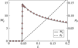
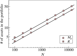
Figure 5: Left: In the case with $m_{i}$ uniformly distributed in $[x-L,x+L]$ we plot the size of the optimal portfolio $M_{T}$ (solid line represents analytical result Eq. (14), symbols are numerical results averaged over $10\,000$ repetitions). With the dashed line the portfolio return $\mu_{P}$ (measured in percents) is shown. The parameters are $N=1\,000$, $D=0.01$, $x=-0.05$. Right: In the case of $N$ assets with $D=0.01$ and $m_{i}$ uniformly distributed in $[0,0.1]$, we plot the average size of the optimal portfolio $M_{T}$, and the inverse participation ratio $\mathcal{R}$. Solid lines are the analytical solutions reported in Eqs. (14) and (15), symbols stand for numerical results.

A more flexible measure of the level of condensation is the inverse participation ratio, defined as $\mathcal{R}=1/\sum_{i=1}^{N}q_{i}^{2}$. It estimates the effective number of assets in the portfolio: when all investment fractions are equal, $\mathcal{R}=N$, while when one asset covers 99% of the portfolio, $\mathcal{R}\approx 1$. Concerning the typical case, using Eq. (9) we can write $\overline{q}_{i}=A-Bi$, $B=(b-a)/[D(N+1)]$, the detailed form of $A$ is not needed for the solution. We assume that the number of profitable assets is larger than the typical size of the optimal portfolio $M_{T}$. Consequently, passing from $i=1$ to $i=M_{T}$, $q_{i}$ decreases linearly to zero and we can use the identity $\sum_{i=1}^{M_{T}}(A-Bi)^{2}=\sum_{i=1}^{M_{T}}(Bi)^{2}$ to obtain

$$\mathcal{R}=\big{[}B^{2}M_{T}(M_{T}+1)(2M_{T}+1)/6\big{]}^{-1}\approx\big{[}B^{2}M_{T}^{3}/3\big{]}^{-1}\approx\tfrac{3}{4}M_{T}.$$ (15)

In the last step we used Eq. (14) for the typical size of the condensed optimal portfolio. We see that the uniform distribution of $m_{i}$ leads to the inverse participation ratio proportional to the number of assets in the portfolio. In the right graph of Fig. 5, Eq. (15) is shown to match the numerical solution (based on Eq. (13)) for various numbers of available assets.

2.4.2 Power-law distribution of $m$

Now we treat the case of a distribution $f(m)$ that has a power-law tail: $f(m)=Cm^{-\alpha-1}$ for $m>m_{\min}$. As long as $M\ll N$, the properties of the assets included in the optimal portfolio are driven by the tail of $f(m)$. In consequence, the detailed form of $f(m)$ for $m<m_{\min}$ is not important here. We assume that only a fraction $r$ of all assets falls in the region $m>m_{\min}$.

Instead of seeking the typical portfolio size $M_{T}$, we shall limit ourselves to finding the conditions when a condensation on one asset arises. With this aim in mind, we put $M=2$ in Eq. (13), obtaining the equation $m_{1}-m_{2}=D$. When $m_{1}-m_{2}>D$, only asset 1 is included in the optimal portfolio. By replacing $m_{1}$ and $m_{2}$ with their medians $\tilde{m}_{1}$ and $\tilde{m}_{2}$, one obtains an approximate condition for a system where such a condensation typically exists. Using order statistics [30] we find the following expressions for the medians: $\tilde{m}_{1}=m_{\min}(Nr/\ln 2)^{1/\alpha}$, $\tilde{m}_{2}\doteq m_{\min}(Nr/1.68)^{1/\alpha}$. The equation $\tilde{m}_{1}-\tilde{m}_{2}=D$ thus achieved can be solved numerically with respect to $\alpha$. In this way we find the value $\alpha_{1}$ below which the optimal portfolio typically contains only the most profitable asset. In Fig. 6 we plot the result as a function of $D$. For comparison, the outcomes from a purely numerical investigation of the equation $P(m_{1}-m_{2}>D)=0.5$ are also shown as filled circles. Our approximate condition has the same qualitative behaviour as the simulation, showing that the use of median gives us a good notion of the optimal portfolio behaviour.

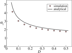
Figure 6: Values of the power law exponent $\alpha_{1}$ at which condensation to one asset arises for $N=1\,000$, $r=0.1$, and $m_{\min}=0.1$. We compare the semi-analytical result obtained by solving $\tilde{m}_{1}-\tilde{m}_{2}=D$ (shown as the solid line) with a numerical simulation of the system (shown as filled circles). Below the line, the optimal portfolio typically contains only one asset.

3 Efficient frontiers

Markowitz’s Efficient Frontier is the line where efficient portfolios are supposed to lie in the Mean-Variance picture. Here we would like to follow the same procedure, using typical instead of average quantities. To capture a typical case, we replace the portfolio return $R_{P}$ by $\ln W_{1}$ in all averages of Sec. 1.2. According to the formula $E((x-E(x))^{2})=E(x^{2})-E(x)^{2}$ we can minimise $E((\ln W_{1})^{2})-E(\ln W_{1})^{2}$ instead of $E((\ln W_{1}-E(\ln W_{1}))^{2})$. With the constraints $E(\ln W_{1})=v_{P}$ and $\sum_{i=1}^{N}q_{i}=1$, the Lagrange function has the form

$$\mathcal{L}=E\big{(}(\ln W_{1})^{2}\big{)}+\gamma_{1}\big{(}E(\ln W_{1})-v_{P}\big{)}+\gamma_{2}\big{(}\sum_{i=1}^{N}q_{i}-1\big{)}.$$ (16)

Its analytical maximisation leads to complicated equations and thus it is convenient to investigate the system numerically; we do so in the particular case of three assets used in Fig. 1. Due to the two constraints there is effectively only one degree of freedom for the minimisation of $E((\ln W_{1})^{2})$ and the numerical procedure may be straightforward.

For the resulting portfolios we can compute expected returns and variances which allows us to add this “Logarithmic Efficient Frontier” (LEF) to the $\sigma_{P}$-$\mu_{P}$ plane depicted in Fig. 1. The result is shown in Fig. 7, where the solid line is again Markowitz’s EF. Solid circles correspond to the three individual assets. The dashed line represents LEF (obtained by the numerical optimisation described above) and the thick gray curve is the region where both EF and LEF consist only of positive portfolio fractions. The solid square represents the Kelly portfolio as follows from Eq. (9) (again, short selling and borrowing are forbidden). We see that EF and LEF are close to each other and thus from the practical point of view they do not differ.

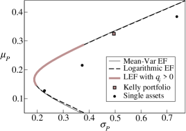
Figure 7: Comparison of two efficient frontiers. The solid line is the classic EF given by Eq. (5). The dashed line is obtained by fixing $E(\ln W_{1})$ and by numerically minimising fluctuations of $\ln W_{1}$ around this value. This we call LEF, its portion with positive $q_{i}$ values is highlighted in thick gray. The small filled circles represent the three individual assets that compose the system. The filled square is the Kelly-optimal portfolio (no borrowing, no short selling).

Finally, let us discuss a useful simplification which allows us, in some cases, to reduce the time-consuming numerical computations. By differentiating Eq. (16) we obtain the condition for the optimal portfolio fractions

$$E\bigg{(}\frac{2\ln W_{1}}{W_{1}}\,R_{i}\bigg{)}+\gamma_{1}\,E\bigg{(}\frac{R_{i}}{W_{1}}\bigg{)}+\gamma_{2}=0\qquad(i=1,\dots,N).$$ (17)

When the parameters of all assets fulfill the condition $m_{i},D_{i}\ll 1$, we can use approximations for $E(R_{i}/W_{1})$ introduced in Appendix A. The first term can be evaluated more precisely using $\ln W_{1}=\ln(1+R_{P})\approx R_{P}$. Hence $E({R_{i}\ln W_{1}}/{W_{1}})\approx q_{i}\,E(R_{i}^{2})+\sum_{j\neq i}q_{j}\,E(R_{i})E(R_{j})$, where $R_{i}=\mathrm{e}^{\eta_{i}}-1$ is the return of asset $i$. Furthermore, for $m_{i},D_{i}\ll 1$ we have $E(R_{i})\approx m_{i}+D_{i}/2$ and $E(R_{i}^{2})\approx D_{i}$. As a result we obtain the equations

$$2q_{i}D_{i}+2(m_{i}+D_{i}/2)\sum_{j\neq i}q_{j}(m_{j}+D_{j}/2)+\gamma_{1}\bigg{[}m_{i}+\frac{D_{i}}{2}\,(1-2q_{i})\bigg{]}+\gamma_{2}=0,$$ (18)

where $i=1,\dots,N$ and the values of $\gamma_{1}$ and $\gamma_{2}$ are fixed by the constraints $\sum_{i=1}^{N}q_{i}(m_{i}+D_{i}/2)=v_{P}$, $\sum_{i=1}^{N}\hat{q}_{i}=1$. This set of $N+2$ nonlinear equations allows us to approximately find Logarithmic Efficient Frontier. In comparison with a straightforward numerical maximisation of Eq. (16) (involving numerical integration of $E(\ln W_{1})$ and $E((\ln W_{1})^{2})$), a substantial saving of computational costs is achieved.

4 Concluding remarks

In this work we investigated the Kelly optimisation strategy in the framework of a simple stochastic model for asset prices. We derived a highly accurate approximate analytical formula for the optimal portfolio fractions. We proved that in the limit of small returns and volatilities of the assets, the constrained Kelly-optimal portfolio lies on the Efficient Frontier. Based on the obtained analytical results, we proposed a simple algorithm for the construction of the optimal portfolio in the constrained case. We showed that since in the investigated case of lognormal returns, Kelly’s approach forbids short positions and borrowing, only a part of the available assets is included in the optimal portfolio. In some cases the size of the optimal portfolio is much smaller than the number of available assets—we say that a portfolio condensation arises. In particular, when the distribution of the mean asset returns is wide, there is a high probability that only the most profitable asset is included in the Kelly-optimal portfolio.

The Mean-Variance analysis is a well-established approach to the portfolio optimisation. We modified this method by replacing the averages $E(W_{1})$ and $E(W_{1}^{2})$ with the logarithm-related quantities $E(\ln W_{1})$ and $E((\ln W_{1})^{2})$. These are less affected by rare events and allow to capture the typical behaviour of the system. As a matter of fact, the difference between the traditional M-V approach and the modification proposed here is very small and does not justify the additional complexity thus induced.

5 Acknowledgement

We acknowledge the partial support from Swiss National Science Foundation (project 205120-113842) as well as STIPCO (European exchange program). We appreciate early collaboration with Dr. Andrea Capocci in this research, stimulating remarks from Damien Challet in late stages of the paper preparation, and helpful comments of our anonymous reviewers.

Appendix A Main approximations

Our aim is to approximate expressions of the type $E(g(\eta))$, where $\eta$ follows a normal distribution $f(\eta)$ with the mean $m$ and the variance $D$. For small values of $D$, this distribution is sharply peaked and an approximate solution can be found expanding $g(\eta)$ around this $m$. This expansion has the following effective form

$$g(\eta)\stackrel{{\scriptstyle\text{ef.}}}{{=}}g(m)+\frac{1}{2}(\eta-m)^{2}g^{(2)}(m)+\frac{1}{24}(\eta-m)^{4}g^{(4)}(x),$$ (19)

for some $x\in[m,\eta]$. Here we dropped the terms proportional to $(\eta-m)^{k}$ with an odd exponent $k$, for they vanish after the averaging. If we take only the first two terms into account, we obtain

$$E\big{(}g(\eta)\big{)}=\int_{-\infty}^{\infty}g(\eta)f(\eta)\,\mathrm{d}\eta\approx g(m)+\frac{D}{2}\,g^{(2)}(m).$$ (20)

This approximation is valid when the following term of the Taylor series brings a negligible contribution $\Delta$. We can estimate it in the following way ($x\in[m,\eta]$)

$$\Delta=\int_{-\infty}^{\infty}\frac{(\eta-m)^{4}}{24}g^{(4)}(x)f(\eta)\,\mathrm{d}\eta\lesssim\int_{-\infty}^{\infty}\frac{(\eta-m)^{4}}{24}\,Mf(\eta)\,\mathrm{d}\eta=\frac{MD^{2}}{8}.$$

Here by $M$ we label the maximum of $\lvert g^{(4)}(\eta)\rvert$ in the region $\mathcal{X}$ where $f(\eta)$ differs from zero considerably, e.g. $\mathcal{X}=[m-2D,m+2D]$. Since $g(x)$ has no singular points in a wide neighbourhood of $m$, its fourth derivative is a bounded and well-behaved function. Thus $M$ is finite and $\Delta$ vanish when $D$ is small.

In particular, in this work we deal with functions of the form $g(\eta_{i})=(\mathrm{e}^{\eta}-1)/[1+q(\mathrm{e}^{\eta}-1)]$. If we use Eq. (20) with this $g(\eta)$, approximate $1+q(\mathrm{e}^{m}-1)$ in the resulting denominators by $1$, $\mathrm{e}^{m}$ by $1$, and $\mathrm{e}^{m}-1$ by $m$, we are left with

$$E\big{(}g(\eta)\big{)}\approx m+D\big{(}1-2q\big{)}/2.$$ (21)

We widely use approximations of this kind to obtain the leading terms for the optimal portfolio fractions in this paper.

Appendix B Procedure for correlated asset prices

So far we have considered uncorrelated asset prices, undergoing the geometric Brownian motion of Eq. (1). Obviously, this is an idealised model and real asset prices exhibit various kinds of correlations. In order to treat correlated prices we employ the covariance matrix $\mathsf{S}$ to characterise the second moment of the stochastic terms $E((\eta_{i}-m_{i})(\eta_{j}-m_{j}))=S_{ij}$. The uncorrelated case can be recovered with the substitution $S_{ij}=\delta_{ij}D_{i}$.

Again, we would like to find an approximation of the term $E\big{(}g(\boldsymbol{\eta})\big{)}\equiv\int g(\boldsymbol{\eta})f(\boldsymbol{\eta})\,\mathrm{d}\boldsymbol{\eta}$. Here $f(\boldsymbol{\eta})$ is the probability distribution of $\boldsymbol{\eta}$ and $g(\boldsymbol{\eta})$ is the function of interest. Notice that the correlations impose the use of vector forms for all the quantities of interest. The Taylor expansion of $g(\boldsymbol{\eta})$ around $\boldsymbol{m}$, Eq. (19) in the uncorrelated case, takes the form

$$g(\boldsymbol{\eta})=g(\boldsymbol{m})+\nabla g(\boldsymbol{m})\cdot(\boldsymbol{\eta}-\boldsymbol{m})+\frac{1}{2}(\boldsymbol{\eta}-\boldsymbol{m})^{T}\mathsf{V}(\boldsymbol{m})(\boldsymbol{\eta}-\boldsymbol{m})+\dots.$$

Here $\mathsf{V}(\boldsymbol{m})$ is the matrix of second derivatives of the function $g(\boldsymbol{\eta})$, calculated at the point $\boldsymbol{\eta}=\boldsymbol{m}$. Now we can proceed in the same way as before

$$E\big{(}g(\boldsymbol{\eta})\big{)} \approx g(\boldsymbol{m})\int f(\boldsymbol{\eta})\,\mathrm{d}\boldsymbol{\eta}+\sum_{i=1}^{N}\partial_{i}g(\boldsymbol{m})\int(\eta_{i}-m_{i})f(\boldsymbol{\eta})\,\mathrm{d}\boldsymbol{\eta}+$$

$$+\frac{1}{2}\sum_{i,j=1}^{N}V_{ij}\int(\eta_{i}-m_{i})(\eta_{j}-m_{j})f(\boldsymbol{\eta})\,\mathrm{d}\boldsymbol{\eta}=$$

$$= g(\boldsymbol{m})+\frac{1}{2}\sum_{i,j=1}^{N}S_{ij}V_{ij}=g(\boldsymbol{m})+\frac{1}{2}\,\mathrm{Tr}(\mathsf{SV}).$$

In the last line we used the symmetry of $\mathsf{S}$. For given $g(\boldsymbol{\eta})$, $\boldsymbol{m}$ and $\mathsf{S}$, we can now solve the equation $E(g(\boldsymbol{\eta}))=0$. In particular, these approximations can be cast into Eq. (6), which can then be treated as in the uncorrelated case.

References

- [1] H. M. Markowitz, The Journal of Finance 7, 77–91, 1952
- [2] W. F. Sharpe, The Journal of Finance 19, 425–442, 1964
- [3] A. F. Perold, Management Science 30, 1143–1160, 1984
- [4] H. Konno and H. Yamazaki, Management Science 37, 519–531, 1991
- [5] E. J. Elton, M. J. Gruber, S. J. Brown, and W. N. Goetzmann, Modern Portfolio Theory and Investment Analysis, 7th Edition, Wiley, 2006
- [6] J. L. Kelly, IEEE Transactions on Information Theory 2, 185–189, 1956
- [7] L. Breiman, Proc. 4th berkeley Symp. Math. Stat. Prob., 65–78, 1962
- [8] M. Finkelstein and R. Whitley, Advances in Applied Probability 13, 415–428, 1981
- [9] S. Browne, in Finding the Edge, Mathematical Analysis of Casino Games, eds. O. Vancura, J. Cornelius, and W. R. Eadington, University of Nevada, 215–231, 2000
- [10] E. O. Thorp, in Handbook of Asset and Liability Management, S. Zenios and W. Ziemba, Eds., Elsevier/North-Holland, 385–428, 2006
- [11] E. Platen and D. Heath, A benchmark approach to quantitative finance, Springer, 2006
- [12] M. Marsili, S. Maslov, and Y.-C. Zhang, Physica A 253, 403–418, 1998
- [13] S. Maslov and Y.-C. Zhang, International Journal of Theoretical and Applied Finance 1, 377–387, 1998
- [14] H. A. Latané, The Journal of Political Economy 67, 144–155, 1959
- [15] P. A. Samuelson, PNAS 68, 2493–2496, 1971
- [16] H. Levy, International Economic Review 14, 601–614, 1973
- [17] H. M. Markowitz, The Journal of Finance 31, 1273–1286, 1976
- [18] L. C. MacLean, W. T. Ziemba, and G. Blazenko, Management Science 38, 1562–1585, 1992
- [19] S. J. Grossman and Z. Zhou, Mathematical Finance 3, 241–276, 1993
- [20] L. C. MacLean and W. T. Ziemba, in Handbook of Asset and Liability Management, S. Zenios and W. Ziemba, Eds., Elsevier/North-Holland, 429–474, 2006
- [21] T. M. Cover and J. A. Thomas, Elements of Information Theory, 2nd Edition, Wiley-Interscience, 2006
- [22] M. Medo, C. H. Yeung, and Y.-C. Zhang, International Review of Financial Analysis 18, 34–39, 2009
- [23] L. C. MacLean, R. Sanegre, Y. Zhao, and W. T. Ziemba, Journal of Economic Dynamics and Control 28, 937–954, 2004
- [24] M. Medo, Y. M. Pis’mak, and Y.-C. Zhang, Physica A 387, 6151–6158, 2008
- [25] R. C. Merton, The Review of Economics and Statistics 51, 247–257, 1969
- [26] S. Browne and W. Whitt, Adv. Appl. Prob. 28, 1145–1176, 1996
- [27] J. Yoshimura and V. A. A. Jansen, Population Ecology 38, 165–182, 1996
- [28] C. T. Bergstrom and M. Lachmann, IEEE Information Theory Workshop 2004, 50–54, 2004
- [29] A. Capocci, private communication
- [30] H. A. David and H. N. Nagaraja, Order Statistics, 3rd Edition, Wiley, 2003